


ABSTRACT
We report here the non-detection of gravitational waves from the merger of binary–neutron star systems and neutron star–black hole systems during the first observing run of the Advanced Laser Interferometer Gravitational-wave Observatory (LIGO). In particular, we searched for gravitational-wave signals from binary–neutron star systems with component masses ![$\in [1,3]\,{M}_{\odot }$](https://content.cld.iop.org/journals/2041-8205/832/2/L21/revision1/apjlaa47c3ieqn1.gif) and component dimensionless spins <0.05. We also searched for neutron star–black hole systems with the same neutron star parameters, black hole mass
and component dimensionless spins <0.05. We also searched for neutron star–black hole systems with the same neutron star parameters, black hole mass ![$\in [2,99]\,{M}_{\odot }$](https://content.cld.iop.org/journals/2041-8205/832/2/L21/revision1/apjlaa47c3ieqn2.gif) , and no restriction on the black hole spin magnitude. We assess the sensitivity of the two LIGO detectors to these systems and find that they could have detected the merger of binary–neutron star systems with component mass distributions of 1.35 ± 0.13 M⊙ at a volume-weighted average distance of ∼70 Mpc, and for neutron star–black hole systems with neutron star masses of 1.4 M⊙ and black hole masses of at least 5 M⊙, a volume-weighted average distance of at least ∼110 Mpc. From this we constrain with 90% confidence the merger rate to be less than 12,600 Gpc−3 yr−1 for binary–neutron star systems and less than 3600 Gpc−3 yr−1 for neutron star–black hole systems. We discuss the astrophysical implications of these results, which we find to be in conflict with only the most optimistic predictions. However, we find that if no detection of neutron star–binary mergers is made in the next two Advanced LIGO and Advanced Virgo observing runs we would place significant constraints on the merger rates. Finally, assuming a rate of
, and no restriction on the black hole spin magnitude. We assess the sensitivity of the two LIGO detectors to these systems and find that they could have detected the merger of binary–neutron star systems with component mass distributions of 1.35 ± 0.13 M⊙ at a volume-weighted average distance of ∼70 Mpc, and for neutron star–black hole systems with neutron star masses of 1.4 M⊙ and black hole masses of at least 5 M⊙, a volume-weighted average distance of at least ∼110 Mpc. From this we constrain with 90% confidence the merger rate to be less than 12,600 Gpc−3 yr−1 for binary–neutron star systems and less than 3600 Gpc−3 yr−1 for neutron star–black hole systems. We discuss the astrophysical implications of these results, which we find to be in conflict with only the most optimistic predictions. However, we find that if no detection of neutron star–binary mergers is made in the next two Advanced LIGO and Advanced Virgo observing runs we would place significant constraints on the merger rates. Finally, assuming a rate of  Gpc−3 yr−1, short gamma-ray bursts beamed toward the Earth, and assuming that all short gamma-ray bursts have binary–neutron star (neutron star–black hole) progenitors, we can use our 90% confidence rate upper limits to constrain the beaming angle of the gamma-ray burst to be greater than
  (
( ).
).
Export citation and abstract BibTeX RIS
1. INTRODUCTION
Between 2015 September 12 and 2016 January 19 the two advanced Laser Interferometer Gravitational-wave Observatory (LIGO) detectors conducted their first observing period (O1). During O1, two high-mass binary black hole (BBH) events were identified with high confidence (>5σ): GW150914 (Abbott et al. 2016i) and GW151226 (Abbott et al. 2016g). A third signal, LVT151012, was also identified with 1.7σ confidence (Abbott et al. 2016c, 2016f) In all three cases, the component masses are confidently constrained to be above the 3.2 M⊙ upper mass limit of neutron stars (NSs) set by theoretical considerations (Rhoades & Ruffini 1974; Abbott et al. 2016j). The details of these observations, investigations about the properties of the observed BBH mergers, and the astrophysical implications are explored in Abbott et al. (2016a, 2016b, 2016c, 2016j, 2016l, 2016m).
The search methods that successfully observed these BBH mergers also target other types of compact binary coalescences (CBCs), specifically the inspiral and merger of neutron star–neutron star (BNS) systems and neutron star–black hole (NSBH) systems. Such systems were considered among the most promising candidates for an observation in O1. For example, a calculation prior to the start of O1 predicted 0.0005–4 detections of BNS signals during O1 (Aasi et al. 2016). Some works, however, predicted that BBH mergers would be the most promising candidates (Dominik et al. 2015; Belczynski et al. 2016; Kinugawa et al. 2016).
In this Letter, we report on the search for BNS and NSBH mergers in O1. We have searched for BNS systems with component masses ![$\in [1,3]\,{M}_{\odot }$](https://content.cld.iop.org/journals/2041-8205/832/2/L21/revision1/apjlaa47c3ieqn6.gif) , component dimensionless spins <0.05, and spin orientations aligned or anti-aligned with the orbital angular momentum. We have searched for NSBH systems with neutron star mass
, component dimensionless spins <0.05, and spin orientations aligned or anti-aligned with the orbital angular momentum. We have searched for NSBH systems with neutron star mass ![$\in [1,3]\,{M}_{\odot }$](https://content.cld.iop.org/journals/2041-8205/832/2/L21/revision1/apjlaa47c3ieqn7.gif) , black hole (BH) mass
, black hole (BH) mass ![$\in [2,99]\,{M}_{\odot }$](https://content.cld.iop.org/journals/2041-8205/832/2/L21/revision1/apjlaa47c3ieqn8.gif) , neutron star dimensionless spin magnitude <0.05, BH dimensionless spin magnitude <0.99, and both spins aligned or anti-aligned with the orbital angular momentum. No observation of either BNS or NSBH mergers was made in O1. We explore the astrophysical implications of this result, placing upper limits on the rates of such merger events in the local universe that are roughly an order of magnitude smaller than those obtained with data from initial LIGO and initial Virgo (Acernese et al. 2008; Abbott et al. 2009; Abadie et al. 2012d). We compare these updated rate limits to current predictions of BNS and NSBH merger rates and explore how the non-detection of BNS and NSBH systems in O1 can be used to explore possible constraints of the opening angle of the radiation cone of short gamma-ray bursts (GRBs), assuming that short GRB progenitors are BNS or NSBH mergers.
, neutron star dimensionless spin magnitude <0.05, BH dimensionless spin magnitude <0.99, and both spins aligned or anti-aligned with the orbital angular momentum. No observation of either BNS or NSBH mergers was made in O1. We explore the astrophysical implications of this result, placing upper limits on the rates of such merger events in the local universe that are roughly an order of magnitude smaller than those obtained with data from initial LIGO and initial Virgo (Acernese et al. 2008; Abbott et al. 2009; Abadie et al. 2012d). We compare these updated rate limits to current predictions of BNS and NSBH merger rates and explore how the non-detection of BNS and NSBH systems in O1 can be used to explore possible constraints of the opening angle of the radiation cone of short gamma-ray bursts (GRBs), assuming that short GRB progenitors are BNS or NSBH mergers.
The layout of this Letter is as follows. In Section 2, we describe the motivation for our search parameter space. In Section 3, we briefly describe the search methodology, then describe the results of the search in Section 4. We then discuss the constraints that can be placed on the rates of BNS and NSBH mergers in Section 5 and the astrophysical implications of the rates in Section 6. Finally, we conclude in Section 7.
2. SOURCE CONSIDERATIONS
There are currently thousands of known NSs, most detected as pulsars (Manchester et al. 2005; Hobbs et al. 2016). Of these, ∼70 are found in binary systems and allow estimates of the NS mass (Lattimer 2012; Antoniadis et al. 2016; Ott et al. 2016; Ozel & Freire 2016). Published mass estimates range from 1.0 ± 0.17 M⊙ (Falanga et al. 2015) to 2.74 ± 0.21 M⊙ (Freire et al. 2008). Considering only precise mass measurements from these observations one can set a lower bound on the maximum possible neutron star mass of 2.01 ± 0.04 M⊙ (Antoniadis et al. 2013) and theoretical considerations set an upper bound on the maximum possible neutron star mass of 2.9–3.2 M⊙ (Rhoades & Ruffini 1974; Kalogera & Baym 1996). The standard formation scenario of core-collapse supernovae restricts the birth masses of neutron stars to be above 1.1 M⊙ (Lattimer 2012; Ozel et al. 2012; Kiziltan et al. 2013).
Several candidate BNS systems allow mass measurements for individual components, giving a much narrower mass distribution (Lorimer 2008). Masses are reported between 1.0 M⊙ and 1.56 M⊙ (Martinez et al. 2015; Ott et al. 2016; Ozel & Freire 2016) and are consistent with an underlying mass distribution of  (Kiziltan et al. 2010). These observational measurements assume masses are greater than 0.9 M⊙.
The fastest spinning pulsar observed so far rotates with a frequency of 716 Hz (Hessels et al. 2006). This corresponds to a dimensionless spin  of roughly 0.4, where m is the object's mass and
  is the angular momentum.141
Such rapid rotation rates likely require the NS to have been spun up through mass transfer from its companion. The fastest spinning pulsar in a confirmed BNS system has a spin frequency of 44 Hz (Kramer & Wex 2009), implying that dimensionless spins for NS in BNS systems are ≤0.04 (Brown et al. 2012). However, recycled NS can have larger spins, and the potential BNS pulsar J1807-2500B (Lynch et al. 2012) has a spin of 4.19 ms, giving a dimensionless spin of up to ∼0.2.142
is the angular momentum.141
Such rapid rotation rates likely require the NS to have been spun up through mass transfer from its companion. The fastest spinning pulsar in a confirmed BNS system has a spin frequency of 44 Hz (Kramer & Wex 2009), implying that dimensionless spins for NS in BNS systems are ≤0.04 (Brown et al. 2012). However, recycled NS can have larger spins, and the potential BNS pulsar J1807-2500B (Lynch et al. 2012) has a spin of 4.19 ms, giving a dimensionless spin of up to ∼0.2.142
Given these considerations, we search for BNS systems with both masses ![$\in [1,3]\,{M}_{\odot }$](https://content.cld.iop.org/journals/2041-8205/832/2/L21/revision1/apjlaa47c3ieqn12.gif) and component dimensionless aligned spins <0.05. We note that some BNS systems with component spins >0.05 are not recovered well when searching only for systems with spins <0.05, as explored in Brown et al. (2012). However, increasing the search space to include BNS systems with larger spins also increases the rate of false alarms. It was found in Nitz (2015) that the overall search sensitivity for BNS systems with spins <0.4 is larger when the search space includes only systems with spins restricted to <0.05 than when the search space is expanded to include spins <0.4.143
and component dimensionless aligned spins <0.05. We note that some BNS systems with component spins >0.05 are not recovered well when searching only for systems with spins <0.05, as explored in Brown et al. (2012). However, increasing the search space to include BNS systems with larger spins also increases the rate of false alarms. It was found in Nitz (2015) that the overall search sensitivity for BNS systems with spins <0.4 is larger when the search space includes only systems with spins restricted to <0.05 than when the search space is expanded to include spins <0.4.143
NSBH systems are thought to be efficiently formed in one of two ways: either through the stellar evolution of field binaries or through dynamical capture of an NS by a BH (Grindlay et al. 2006; Sadowski et al. 2008; Lee et al. 2010; Benacquista & Downing 2013). Though no NSBH systems are known to exist, likely progenitors have been observed, Cyg X-3 (Belczynski et al. 2013; Casares et al. 2014; Grudzinska et al. 2015).
Measurements of galactic stellar-mass BHs in X-ray binaries yield BH masses 5 ≤ MBH/M⊙ ≤ 24 (Merloni 2008; Ozel et al. 2010; Farr et al. 2011; Wiktorowicz et al. 2013; also see the table in Wiktorowicz & Belcynski 2016, for a full list of citations for BH mass measurements). Extragalactic high-mass X-ray binaries, such as IC10 X-1 and NGC300 X-1 suggest BH masses of 20–30 M⊙. Advanced LIGO has observed two definitive BBH systems and constrained the masses of the four component BHs to  and
and  , respectively, and the masses of the two resulting BHs to
  and
and  . In addition, if one assumes that the candidate BBH merger LVT151012 was of astrophysical origin, then its component BHs had masses constrained to
  and
and  with a resulting BH mass of
  . There is an apparent gap of BHs in the mass range 3–5 M⊙, which has been ascribed to the supernova explosion mechanism (Belczynski et al. 2012; Fryer et al. 2012). However, BHs formed from stellar evolution may exist with masses down to 2 M⊙, especially if they are formed from matter accreted onto neutron stars (O'Shaughnessy et al. 2005a). Depending on the amount of mass lost in stellar winds, isolated and binary star evolution models typically allow for stellar-mass BH up to ∼80–100 M⊙ (see, e.g., Woosley et al. 2002; Heger et al. 2003; Belczynski et al. 2010; Dominik et al. 2012; Fryer et al. 2012 and references therein); stellar BHs with mass above 100 M⊙ are also conceivable (Belczynski et al. 2014; de Mink & Belczynski 2015), possibly separated from the low-mass region due to the effects of pair-instability supernovae (Woosley et al. 2002; Chen et al. 2014; Marchant et al. 2016).
X-ray observations of accreting BHs indicate a broad distribution of BH spin (Li et al. 2005; Davis et al. 2006; McClintock et al. 2006; Shafee et al. 2006; Liu et al. 2008; Gou et al. 2009; Miller et al. 2009; Miller & Miller 2014). Some BHs observed in X-ray binaries have very large dimensionless spins (e.g Cygnus X-1 at >0.95; Gou et al. 2011; Fabian et al. 2012), while others could have much lower spins (∼0.1; McClintock et al. 2011). Measured BH spins in high-mass X-ray binary systems tend to have large values (>0.85), and these systems are more likely to be progenitors of NSBH binaries (McClintock et al. 2014). Isolated BH spins are only constrained by the relativistic Kerr bound χ ≤ 1 (Misner et al. 1973). LIGO's observations of merging binary BH systems yield weak constraints on component spins (Abbott et al. 2016c, 2016g, 2016j). The microquasar XTE J1550-564 (Steiner & McClintock 2012) and population synthesis models(Fragos et al. 2010) indicate small spin–orbit misalignment in field binaries. Dynamically formed NSBH systems, in contrast, are expected to have no correlation between the spins and the orbit.
We search for NSBH systems with NS mass ![$\in [1,3]\,{M}_{\odot }$](https://content.cld.iop.org/journals/2041-8205/832/2/L21/revision1/apjlaa47c3ieqn20.gif) , NS dimensionless spins <0.05, BH mass
, NS dimensionless spins <0.05, BH mass ![$\in [2,99]\,{M}_{\odot }$](https://content.cld.iop.org/journals/2041-8205/832/2/L21/revision1/apjlaa47c3ieqn21.gif) , and BH spin magnitude <0.99. Current search techniques are restricted to waveform models where the spins are (anti-)aligned with the orbit (Usman et al. 2016; Messick et al. 2016), although methods to extend this to generic spins are being explored (Harry et al. 2016). Nevertheless, aligned-spin searches have been shown to have good sensitivity to systems with generic spin orientations in O1 (Dal Canton et al. 2015; Harry et al. 2016). An additional search for BBH systems with total mass greater than 100 M⊙ is also being performed, the results of which will be reported in a future publication.
, and BH spin magnitude <0.99. Current search techniques are restricted to waveform models where the spins are (anti-)aligned with the orbit (Usman et al. 2016; Messick et al. 2016), although methods to extend this to generic spins are being explored (Harry et al. 2016). Nevertheless, aligned-spin searches have been shown to have good sensitivity to systems with generic spin orientations in O1 (Dal Canton et al. 2015; Harry et al. 2016). An additional search for BBH systems with total mass greater than 100 M⊙ is also being performed, the results of which will be reported in a future publication.
3. SEARCH DESCRIPTION
To observe CBCs in data taken from Advanced LIGO we use matched-filtering against models of compact binary merger gravitational-wave (GW) signals (Wainstein & Zubakov 1962). Matched-filtering has long been the primary tool for modeled GW searches (Abbott et al. 2004; Abadie et al. 2012d). As the emitted GW signal varies significantly over the range of masses and spins in the BNS and NSBH parameter space, the matched-filtering process must be repeated over a large set of filter waveforms, or "template bank" (Owen & Sathyaprakash 1999). The ranges of masses considered in the searches are shown in Figure 1. The matched-filter process is conducted independently for each of the two LIGO observatories before searching for any potential GW signals observed at both observatories with the same masses and spins and within the expected light travel time delay. A summary statistic is then assigned to each coincident event based on the estimated rate of false alarms produced by the search background that would be more significant than the event.

Figure 1. Range of template mass parameters considered for the three different template banks used in the search. The offline analyses and online GstLAL after 2015 December 23 used the largest bank up to total masses of 100 M⊙. The online mbta bank covered primary masses below 12 M⊙ and chirp masses (see footnote 143) below 5 M⊙. The early online GstLAL bank up to 2015 December 23 covered primary masses up to 16 M⊙ and secondary masses up to 2.8 M⊙. The spin ranges are not shown here but are discussed in the text.
Download figure:
Standard image High-resolution imageBNS and NSBH mergers are prime candidates not only for observation with GW facilities, but also for coincident observation with electromagnetic (EM) observatories (Eichler et al. 1989; Narayan et al. 1992; Li & Paczynski 1998; Hansen & Lyutikov 2001; Nakar 2007; Nakar & Piran 2011; Metzger & Berger 2012; Berger 2014; Zhang 2014; Fong et al. 2015). We have a long history of working with the Fermi, Swift, and IPN GRB teams to perform sub-threshold searches of GW data in a narrow window around the time of observed GRBs (Abbott et al. 2005, 2008; Abadie et al. 2012b, 2012c). Such a search is currently being performed on O1 data and will be reported in a forthcoming publication. In O1 we also aimed to rapidly alert EM partners if a GW observation was made (Abbott et al. 2016h). Therefore, it was critical for us to rapidly search for compact coalescences in our data to identify potential BNS or NSBH mergers within a timescale of minutes after the data is taken, thereby giving EM partners the best chance to perform a coincident observation. We refer to this as our "online" search.
Nevertheless, analyses running with minute latency do not have access to full data-characterization studies, which can take weeks to perform, or to data with the most complete knowledge about calibration and associated uncertainties. Additionally, in rare instances, online analyses may fail to analyze stretches of data due to computational failure. Therefore, it is also important to have an "offline" search, which performs the most sensitive search possible for BNS and NSBH sources. We give here a brief description of both the offline and online searches, referring to other works to give more details when relevant.
3.1. Offline Search
The offline CBC search of the O1 data set consists of two independently implemented matched-filter analyses: GstLAL(Messick et al. 2016) and PyCBC (Usman et al. 2016). For detailed descriptions of these analyses and associated methods we refer the reader to Allen (2005), Allen et al. (2012), Babak et al. (2013), Dal Canton et al. (2014), and Usman et al. (2016) for PyCBC and Cannon et al. (2012, 2013), Privitera et al. (2014), and Messick et al. (2016) for GstLAL. We also refer the reader to Abbott et al. (2016c, 2016f) for a detailed description of the offline search of the O1 data set; here, we give only a brief overview.
In contrast to the online search, the offline search uses data produced with smaller calibration errors (Abbott et al. 2016d), uses complete information about the instrumental data quality (Abbott et al. 2016e), and ensures that all available data is analyzed. The offline search in O1 forms a single search targeting BNS, NSBH, and BBH systems. The waveform filters cover systems with individual component masses ranging from 1 to 99 M⊙, total mass constrained to less than 100 M⊙ (see Figure 1), and component dimensionless spins up to ± 0.05 for components with mass less than 2 M⊙ and ±0.99 otherwise (Abbott et al. 2016c; Capano et al. 2016). Waveform filters with total mass less than 4 M⊙ (chirp mass less than 1.73 M⊙144 ) for PyCBC (GstLAL) are modeled with the inspiral-only, post-Newtonian, frequency-domain approximant "TaylorF2" (Arun et al. 2009; Bohé et al. 2013, 2015; Blanchet 2014; Mishra et al. 2016). At larger masses, it becomes important to also include the merger and ringdown components of the waveform. There a reduced-order model of the effective-one-body waveform calibrated against numerical relativity is used (Taracchini et al. 2014; Pürrer 2016).
3.2. Online Search
The online compact binary coalescence (CBC) search of the O1 data also consisted of two analyses; an online version of GstLAL (Messick et al. 2016) and mbta (Adams et al. 2016). For detailed descriptions of the mbta analysis we refer the reader to Beauville et al. (2008), Abadie et al. (2012a), and Adams et al. (2016). The bank of waveform filters used by GstLAL up to 2015 December 23—and by mbta for the duration of O1—targeted systems that contained at least one NS. Such systems are most likely to have an EM counterpart, which would be powered by the material from a disrupted NS. These sets of waveform filters were constructed using methods described in Brown et al. (2012), Harry et al. (2014), and Pannarale & Ohme (2014). GstLAL chose to cover systems with component masses of ![${m}_{1}\in [1,16]\,{M}_{\odot };{m}_{2}\in [1,2.8]\,{M}_{\odot }$](https://content.cld.iop.org/journals/2041-8205/832/2/L21/revision1/apjlaa47c3ieqn23.gif) and mbta covered
and mbta covered ![${m}_{1},{m}_{2}\in [1,12]\,{M}_{\odot }$](https://content.cld.iop.org/journals/2041-8205/832/2/L21/revision1/apjlaa47c3ieqn24.gif) with a limit on chirp mass
with a limit on chirp mass  (see Figure 1). In GstLAL, component spins were limited to χi < 0.05 for mi < 2.8 M⊙ and χi < 1 otherwise, for mbta χi < 0.05 for mi < 2 M⊙ and χi < 1 otherwise. GstLAL also chose to limit the template bank to include only systems for which it is possible for an NS to have disrupted during the late inspiral using constraints described in Pannarale & Ohme (2014). For the mbta search the waveform filters were modeled using the "TaylorT4" time-domain, post-Newtonian inspiral approximant (Buonanno et al. 2009). For GstLAL the TaylorF2 frequency-domain, post-Newtonian waveform approximant was used (Arun et al. 2009; Bohé et al. 2013, 2015; Blanchet 2014; Mishra et al. 2016). All waveform models used in this paper are publicly available in the lalsimulation repository (Mercer et al. 2016).145
After 2015 December 23, and triggered by the discovery of GW150914, the GstLAL analysis was extended to cover the same search space—using the same set of waveform filters—as the offline search (Abbott et al. 2016c; Capano et al. 2016).
3.3. Data Set
Advanced LIGO's first observing run occurred between 2015 September 12 and 2016 January 19 and consists of data from the two LIGO observatories in Hanford, WA, and Livingston, LA. The LIGO detectors were running stably with roughly 40% coincident operation and had been commissioned to roughly one-third of the design sensitivity by the time of the start of O1 (Martynov et al. 2016). During this observing run, the final offline data set consisted of 76.7 days of data from the Hanford observatory and 65.8 days of data from the Livingston observatory. We analyze only times during which both observatories took data, which is 49.0 days. Characterization studies of the data set found 0.5 days of coincident data during which time there was some identified instrumental problem—known to introduce excess noise—in at least one of the interferometers (Abbott et al. 2016e). These times are removed before assessing the significance of events in the remaining analysis time. Some additional time is not analyzed because of restrictions on the minimal length of data segments and because of data lost at the start and end of those segments (Abbott et al. 2016c, 2016f). These requirements are slightly different between the two offline analyses, and PyCBC analyzed 46.1 days of data while GstLAL analyzed 48.3 days of data.
The data available to the online analyses are not exactly the same as that available to the offline analyses. Some data were not available online due to (for example) software failures and can later be made available for offline analysis. In contrast, some data identified as analyzable for the online codes may later be identified as invalid as the result of updated data-characterization studies or because of problems in the calibration of the data. During O1, a total of 52.2 days of coincident data was made available for online analysis. Of this coincident online data, mbta analyzed 50.5 days (96.6%) and GstLAL analyzed 49.4 days (94.6%). A total of 52.0 days (99.5%) of data was analyzed by at least one of the online analyses.
4. SEARCH RESULTS
The offline search, targeting BBH as well as BNS and NSBH mergers, found three significant events during O1. Two signals were recovered with >5σ confidence (Abbott et al. 2016g, 2016i) and a third signal was found with 1.7σ confidence (Abbott et al. 2016c, 2016f). Subsequent parameter inference on all three of these events has determined that, to very high confidence, they were not produced by a BNS or NSBH merger (Abbott et al. 2016c, 2016j). No other events are significant with respect to the noise background in the offline search (Abbott et al. 2016c), and we therefore state that no BNS or NSBH mergers were observed.
The online search identified a total of eight unique GW candidate events with a false-alarm rate (FAR) less than 6 yr−1. Events with an FAR less than this are sent to electromagnetic partners if they pass event validation. Six of the events were rejected during the event validation as they were associated with known non-Gaussian behavior in one of the observatories. Of the remaining events, one was the BBH merger GW151226 reported in Abbott et al. (2016g). The second event identified by GstLAL was only narrowly below the FAR threshold, with an FAR of 3.1 yr−1. This event was also detected by mbta with a higher FAR of 35 yr−1. This is consistent with noise in the online searches and the candidate event was later identified to have a false-alarm rate of 190 yr−1 in the offline GstLAL analysis. Nevertheless, the event passed all event validation and was released for EM follow-up observations, which showed no significant counterpart. The results of the EM follow-up program are discussed in more detail in Abbott et al. (2016h).
All events identified by the GstLAL or mbta online analyses with a false-alarm rate of less than 3200 yr−1 are uploaded to an internal database known as the gravitational-wave candidate event database (GraCEDb; Moe et al. 2016). In total, 486 events were uploaded from mbta and 868 from GstLAL. We can measure the latency of the online pipelines from the time between the inferred arrival time of each event at the Earth and the time at which the event is uploaded to GraCEDb. This latency is illustrated in Figure 2, where it can be seen that both online pipelines achieved median latencies on the order of one minute. We note that GstLAL uploaded twice as many events as mbta because of a difference in how the FAR was defined. The FAR reported by mbta was defined relative to the rate of coincident data such that an event with an FAR of 1 yr−1 is expected to occur once in a year of coincident data. The FAR reported by GstLAL was defined relative to wall-clock time such that an event with an FAR of 1 yr−1 is expected to occur once in a calendar year. In the following section, we use the mbta definition of FAR when computing rate upper limits.

Figure 2. Latency of the online searches during O1. The latency is measured as the time between the event arriving at Earth and time at which the event is uploaded to GraCEDb.
Download figure:
Standard image High-resolution image5. RATES
5.1. Calculating Upper Limits
Given no evidence for BNS or NSBH coalescences during O1, we seek to place an upper limit on the astrophysical rate of such events. The expected number of observed events Λ in a given analysis can be related to the astrophysical rate of coalescences for a given source R by

Here,  is the spacetime volume that the detectors are sensitive to—averaged over space, observation time, and the parameters of the source population of interest, which we describe in detail later in this section. The likelihood for finding zero observations in the data s follows the Poisson distribution for zero events
  . Bayes' theorem then gives the posterior for Λ

where p(Λ) is the prior on Λ.
Searches of initial LIGO and initial Virgo data used a uniform prior on Λ (Abadie et al. 2012d) but included prior information from previous searches. For the O1 BBH search, however, a Jeffreys prior of  for the Poisson likelihood was used (Farr et al. 2015; Abbott et al. 2016c, 2016m). A Jeffreys prior has the convenient property that the resulting posterior is invariant under a change in parameterization. However, for consistency with past BNS and NSBH results we will primarily use a uniform prior. In a Poisson posterior, a prior
  produces a posterior mean that is
  , where Nobs is the number of observed events (zero in our case). Common choices for α are α = 0 (flat; as we use here), α = 1/2 (Jeffreys; as used in Abbott et al. 2016c, 2016m), and α = 1 (flat in
  this prior produces an improper posterior for our situation of zero observations, and therefore is not appropriate here). The choice of α involves a trade off between formal unbiasedness (
 ), achieved by the α = 1 prior, and applicability in the Nobs = 0 case.
We do not include additional prior information from past observations because the sensitive  from all previous runs is an order of magnitude smaller than that of O1. We estimate
  by adding a large number of simulated waveforms sampled from an astrophysical population into the data. These simulated signals are recovered with an estimate of the FAR using the offline analyses. Monte Carlo integration methods are then utilized to estimate the sensitive volume to which the detectors can recover gravitational-wave signals below a chosen FAR threshold, which in this Letter we choose to be 0.01 yr−1. This threshold is low enough that only signals that are likely to be true events are counted as found, and we note that varying this threshold in the range 0.0001–1 yr−1 only changes the calculated
  by about ±20%.
Calibration uncertainties lead to a difference between the amplitude of simulated waveforms and the amplitude of real waveforms with the same luminosity distance dL. During O1, the 1σ uncertainty in the strain amplitude was 6%, resulting in an 18% uncertainty in the measured  . Results presented here also assume that injected waveforms are accurate representations of astrophysical sources. We use a time-domain, aligned-spin, post-Newtonian point-particle approximant to model BNS injections (Buonanno et al. 2009), and a time-domain, effective-one-body waveform calibrated against numerical relativity to model NSBH injections (Pan et al. 2014; Taracchini et al. 2014). Waveform differences between these models and the offline search templates are therefore including in the calculated
  . The injected NSBH waveform model is not calibrated at high mass ratios (m1/m2 > 8), so there is some additional modeling uncertainty for large-mass NSBH systems. The true sensitive volume
  will also be smaller if the effect of tides in BNS or NSBH mergers is extreme. However, for most scenarios the effects of waveform modeling will be smaller than the effects of calibration errors and the choice of prior discussed above.
The posterior on Λ (Equation (2)) can be reexpressed as a joint posterior on the astrophysical rate R and the sensitive volume 

The new prior can be expanded as  . For
. For  , we will either use a uniform prior on R or a prior proportional to the Jeffreys prior
  . As with Abbott et al. (2016c, 2016k, 2016m), we use a log-normal prior on

where μ is the calculated value of  and σ represents the fractional uncertainty in
  . Below, we will use an uncertainty of σ = 18% due mainly to calibration errors.
Finally, a posterior for the rate is obtained by marginalizing over  ,
,

The upper limit Rc on the rate with confidence c is then given by the solution to

For reference, we note that in the limit of zero uncertainty in  , the uniform prior for
  gives a rate upper limit of
corresponding to  for a 90% confidence upper limit (Biswas et al. 2009). For a Jeffreys prior on
  , this upper limit is
corresponding to  for a 90% confidence upper limit.
5.2. BNS Rate Limits
Motivated by considerations in Section 2, we begin by considering a population of BNS sources with a narrow range of component masses sampled from the normal distribution  and truncated to remove samples outside the range [1, 3] M⊙. We consider both a "low spin" BNS population, where spins are distributed with uniform dimensionless spin magnitude
 ![$\in [0,0.05]$](https://content.cld.iop.org/journals/2041-8205/832/2/L21/revision1/apjlaa47c3ieqn53.gif) and isotropic direction, and a "high spin" BNS population with a uniform dimensionless spin magnitude
and isotropic direction, and a "high spin" BNS population with a uniform dimensionless spin magnitude ![$\in [0,0.4]$](https://content.cld.iop.org/journals/2041-8205/832/2/L21/revision1/apjlaa47c3ieqn54.gif) and isotropic direction. Our population uses an isotropic distribution of sky location and source orientation and chooses distances assuming a uniform distribution in volume. These simulations are modeled using a post-Newtonian waveform model, expanded using the "TaylorT4" formalism (Buonanno et al. 2009). From this population we compute the spacetime volume that Advanced LIGO was sensitive to during the O1 observing run. Results are shown for the measured
and isotropic direction. Our population uses an isotropic distribution of sky location and source orientation and chooses distances assuming a uniform distribution in volume. These simulations are modeled using a post-Newtonian waveform model, expanded using the "TaylorT4" formalism (Buonanno et al. 2009). From this population we compute the spacetime volume that Advanced LIGO was sensitive to during the O1 observing run. Results are shown for the measured  in Table 1 using a detection threshold of FAR = 0.01 yr−1. Because the template bank for the searches use only aligned-spin BNS templates with component spins up to 0.05, the PyCBC (GstLAL) pipelines are 4% (6%) more sensitive to the low-spin population than to the high-spin population. The difference in
  between the two analyses is no larger than 6%, which is consistent with the difference in time analyzed in the two analyses. In addition, the calculated
  has a Monte Carlo integration uncertainty of ∼1.5% due to the finite number of injection samples.
Table 1.
Sensitive Spacetime Volume  and 90% Confidence Upper Limit R90% for BNS Systems
| Injection | Range of Spin |
 (Gpc3 yr) (Gpc3 yr) |
Range (Mpc) | R90% (Gpc−3 yr−1) | |||
|---|---|---|---|---|---|---|---|
| Set | Magnitudes | PyCBC | GstLAL | PyCBC | GstLAL | PyCBC | GstLAL |
| Isotropic low spin | [0, 0.05] | 2.09 × 10⁻⁴ | 2.21 × 10⁻⁴ | 73.2 | 73.6 | 12,100 | 11,400 |
| Isotropic high spin | [0, 0.4] | 2.00 × 10⁻⁴ | 2.08 × 10⁻⁴ | 72.1 | 72.1 | 12,600 | 12,100 |
Note. Component masses are sampled from a normal distribution  ) with samples outside the range [1, 3] M⊙ removed. Values are shown for both the pycbc and gstlal pipelines.
  is calculated using an FAR threshold of 0.01 yr−1. The rate upper limit is calculated using a uniform prior on
  and an 18% uncertainty in
  from calibration errors.
Download table as: ASCIITypeset image
Using the measured  , the rate posterior and upper limit can be calculated from Equations (5) and (6), respectively. The posterior and upper limits are shown in Figure 3 and depend sensitively on the choice of uniform versus Jeffreys prior for
  . However, they depend only weakly on the spin distribution of the BNS population and on the width σ of the uncertainty in
  . For the conservative uniform prior on Λ and an uncertainty in
  due to calibration errors of 18%, we find the 90% confidence upper limit on the rate of BNS mergers to be 12,100 Gpc−3 yr−1 for low spin and 12,600 Gpc−3 yr−1 for high spin using the values of
  calculated with PyCBC; results for GstLAL are also shown in Table 1. These numbers can be compared to the upper limit computed from analysis of Initial LIGO and Initial Virgo data (Abadie et al. 2012d). There, the upper limit for 1.35–1.35 M⊙ non-spinning BNS mergers is given as 130,000 Gpc−3 yr−1. The O1 upper limit is more than an order of magnitude lower than this previous upper limit.

Figure 3. Posterior density on the rate of BNS mergers calculated using the PyCBC analysis. Blue curves represent a uniform prior on the Poisson parameter  , while green curves represent a Jeffreys prior on Λ. The solid (low spin population) and dotted (high spin population) posteriors almost overlap. The vertical dashed and solid lines represent the 50% and 90% confidence upper limits, respectively, for each choice of prior on Λ. For each pair of vertical lines, the left line is the upper limit for the low spin population and the right line is the upper limit for the high spin population. Also shown are the realistic Rre and high-end Rhigh of the expected BNS merger rates identified in Abadie et al. (2010).
Download figure:
Standard image High-resolution imageTo allow for uncertainties in the mass distribution of BNS systems we also derive 90% confidence upper limits as a function of the NS component masses. To do this, we construct a population of software injections with component masses sampled uniformly in the range [1, 3] M⊙ and an isotropic distribution of component spins with magnitudes uniformly distributed in [0, 0.05]. We then bin the BNS injections by mass and calculate  and the associated 90% confidence rate upper limit for each bin. The 90% rate upper limit for the conservative uniform prior on Λ as a function of component masses is shown in Figure 4 for PyCBC. The fractional difference between the PyCBC and GstLAL results ranges from 1% to 16%.
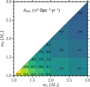
Figure 4. 90% confidence upper limit on the BNS merger rate as a function of the two component masses using the PyCBC analysis. Here, the upper limit for each bin is obtained assuming a BNS population with masses distributed uniformly within the limits of each bin, considering isotropic spin direction and dimensionless spin magnitudes uniformly distributed in [0, 0.05].
Download figure:
Standard image High-resolution image5.3. NSBH Rate Limits
Given the absence of known NSBH systems and uncertainty in the BH mass, we evaluate the rate upper limit for a range of BH masses. We use three masses that span the likely range of BH masses: 5 M⊙, 10 M⊙, and 30 M⊙. For the NS mass, we use the canonical value of 1.4 M⊙. We assume a distribution of BH spin magnitudes uniform in [0, 1] and NS spin magnitudes uniform in [0, 0.04]. For these three mass pairs, we compute upper limits for an isotropic spin distribution on both bodies, and for a case where both spins are aligned or anti-aligned with the orbital angular momentum (with equal probability of aligned versus anti-aligned). Our NSBH population uses an isotropic distribution of sky location and source orientation and chooses distances assuming a uniform distribution in volume. Waveforms are modeled using the spin-precessing, effective-one-body model calibrated against numerical relativity waveforms described in Taracchini et al. (2014) and Babak et al. (2016).
The measured  for an FAR threshold of 0.01 yr−1 is given in Table 2 for PyCBC and GstLAL. The uncertainty in the Monte Carlo integration of
  is 1.5%–2%. The corresponding 90% confidence upper limits are also given using the conservative uniform prior on Λ and an 18% uncertainty in
  . Analysis-specific differences in the limits range from 1% to 20%, comparable or less than other uncertainties such as calibration. These results can be compared to the upper limits found for initial LIGO and Virgo for a population of 1.35 M⊙–5 M⊙ NSBH binaries with isotropic spin of 36,000 Gpc−3 yr−1 at 90% confidence (Abadie et al. 2012d). As with the BNS case, this is an improvement in the upper limit of over an order of magnitude.
Table 2.
Sensitive Spacetime Volume  and 90% Confidence Upper Limit R90% for NSBH Systems with Isotropic and Aligned-spin Distributions
| NS mass | BH mass | Spin |
 (Gpc3 yr) (Gpc3 yr) |
Range (Mpc) | R90% (Gpc−3 yr−1) | |||
|---|---|---|---|---|---|---|---|---|
| (M⊙) | (M⊙) | distribution | PyCBC | GstLAL | PyCBC | GstLAL | PyCBC | GstLAL |
| 1.4 | 5 | Isotropic | 7.01 × 10⁻⁴ | 7.75 × 10⁻⁴ | 110 | 112 | 3600 | 3260 |
| 1.4 | 5 | Aligned | 7.87 × 10⁻⁴ | 9.01 × 10⁻⁴ | 114 | 118 | 3210 | 2800 |
| 1.4 | 10 | Isotropic | 1.00 × 10⁻³ | 1.02 × 10⁻³ | 123 | 122 | 2530 | 2480 |
| 1.4 | 10 | Aligned | 1.36 × 10⁻³ | 1.53 × 10⁻³ | 137 | 140 | 1850 | 1650 |
| 1.4 | 30 | Isotropic | 1.10 × 10⁻³ | 9.12 × 10⁻⁴ | 127 | 118 | 2300 | 2770 |
| 1.4 | 30 | Aligned | 1.98 × 10⁻³ | 2.01 × 10⁻³ | 155 | 154 | 1280 | 1260 |
Note. The NS spin magnitudes are in the range [0, 0.04] and the BH spin magnitudes are in the range [0, 1]. Values are shown for both the pycbc and gstlal pipelines.  is calculated using an FAR threshold of 0.01 yr−1. The rate upper limit is calculated using a uniform prior on
  and an 18% uncertainty in
  from calibration errors.
Download table as: ASCIITypeset image
We also plot the 50% and 90% confidence upper limits from PyCBC and GstLAL as a function of mass in Figure 5 for the uniform prior. The search is less sensitive to isotropic spins than to (anti-)aligned spins due to two factors. First, the volume-averaged signal power is larger for a population of (anti-)aligned-spin systems than for isotropic spin systems. Second, the search uses a template bank of (anti-)aligned-spin systems, and thus loses sensitivity when searching for systems with significantly misaligned spins. As a result, the rate upper limits are less constraining for the isotropic spin distribution than for the (anti-)aligned-spin case.

Figure 5. 50% and 90% upper limits on the NSBH merger rate as a function of the BH mass using the more conservative uniform prior for the counts Λ. Blue curves represent the PyCBC analysis, and red curves represent the GstLAL analysis. The NS mass is assumed to be 1.4 M⊙. The spin magnitudes were sampled uniformly in the range [0, 0.04] for NSs and [0, 1] for BHs. For the aligned-spin injection set, the spins of both the NS and BH are aligned (or anti-aligned) with the orbital angular momentum. For the isotropic spin injection set, the orientation for the spins of both the NS and BH are sampled isotropically. The isotropic spin distribution results in a larger upper limit. Also shown are the realistic Rre and high-end Rhigh of the expected NSBH merger rates identified in Abadie et al. (2010).
Download figure:
Standard image High-resolution image6. ASTROPHYSICAL INTERPRETATION
We can compare our upper limits with rate predictions for compact object mergers involving NSs, shown for BNS in Figure 6 and for NSBH in Figure 7. A wide range of predictions derived from population synthesis and from binary pulsar observations were reviewed in 2010 to produce rate estimates for canonical 1.4 M⊙ NSs and 10 M⊙ BHs (Abadie et al. 2010). We additionally include some more recent estimates from population synthesis for both NSBH and BNS (de Mink & Belczynski 2015; Dominik et al. 2015; Belczynski et al. 2016; keeping in mind these calculations do not simultaneously and widely explore all uncertainties in binary evolution, hence underestimating the underlying uncertainties; cf. O'Shaughnessy et al. 2005b, 2008, 2010, and references therein) and binary pulsar observations for BNS (Kim et al. 2015). Finally, to give a sense of scale to the results shown in Figures 6 and 7, we note that the core-collapse supernova rate, in these units, is ∼105 Gpc−3 yr−1 (Cappellaro et al. 2015 and references therein).
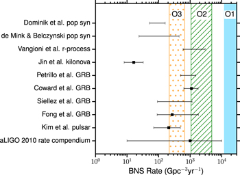
Figure 6. Comparison of the O1 90% upper limit on the BNS merger rate to other rates discussed in the text (Abadie et al. 2010; Coward et al. 2012; Petrillo et al. 2013; Siellez et al. 2014; de Mink & Belczynski 2015; Dominik et al. 2015; Fong et al. 2015; Jin et al. 2015; Kim et al. 2015; Vangioni et al. 2016). The region excluded by the low-spin BNS rate limit is shaded in blue. Continued non-detection in O2 (slash) and O3 (dot) with higher sensitivities and longer operation time would imply stronger upper limits. The O2 and O3 BNS ranges are assumed to be 1–1.9 and 1.9–2.7 times larger than O1. The operation times are assumed to be 6 and 9 months (Aasi et al. 2016) with a duty cycle equal to that of O1 (∼40%). For comparison the core-collapse supernova rate in these units is ∼105 Gpc−3 yr−1 (Cappellaro et al. 2015 and references therein).
Download figure:
Standard image High-resolution image
Figure 7. Comparison of the O1 90% upper limit on the NSBH merger rate to other rates discussed in the text (Abadie et al. 2010; Coward et al. 2012; Petrillo et al. 2013; Dominik et al. 2015; de Mink & Belczynski 2015; Fong et al. 2015; Jin et al. 2015; Vangioni et al. 2016). The dark blue region assumes an NSBH population with masses 5–1.4 M⊙, and the light blue region assumes an NSBH population with masses 10–1.4 M⊙. Both assume an isotropic spin distribution. Continued non-detection in O2 (slash) and O3 (dot) with higher sensitivities and longer operation time would imply stronger upper limits (shown for 10–1.4 M⊙ NSBH systems). The O2 and O3 ranges are assumed to be 1–1.9 and 1.9–2.7 times larger than O1. The operation times are assumed to be 6 and 9 months (Aasi et al. 2016) with a duty cycle equal to that of O1 (∼40%). For comparison the core-collapse supernova rate in these units is ∼105 Gpc−3 yr−1 (Cappellaro et al. 2015 and references therein).
Download figure:
Standard image High-resolution imageWe also compare our upper limits for NSBH and BNS systems to beaming-corrected estimates of short GRB rates in the local universe. Short GRBs are considered likely to be produced by the merger of compact binaries that include NSs, i.e., BNS or NSBH systems (Berger 2014). The rate of short GRBs can predict the rate of progenitor mergers (Coward et al. 2012; Petrillo et al. 2013; Siellez et al. 2014; Fong et al. 2015). For NSBH, systems with small BH masses are considered more likely to be able to produce short GRBs (e.g. Duez 2010; Giacomazzo et al. 2013; Pannarale et al. 2015), so we compare to our 5 M⊙–1.4 M⊙ NSBH rate constraint. The observation of a kilonova is also considered to be an indicator of a binary merger (Metzger & Berger 2012), and an estimated kilonova rate gives an additional lower bound on compact binary mergers (Jin et al. 2015).
Finally, some recent work has used the idea that mergers involving NSs are the primary astrophysical source of r-process elements (Lattimer & Schramm 1974; Qian & Wasserburg 2007) to constrain the rate of such mergers from nucleosynthesis (Bauswein et al. 2014; Vangioni et al. 2016), and we include rates from Vangioni et al. (2016) for comparison.
While limits from O1 are not yet in conflict with astrophysical models, scaling our results to current expectations for advanced LIGO's next two observing runs, O2 and O3 (Aasi et al. 2016), suggests that significant constraints or observations of BNS or NSBH mergers are possible in the next two years.
Assuming that short GRBs are produced by BNS or NSBH, but without using beaming angle estimates, we can constrain the beaming angle of the jet of gamma rays emitted from these GRBs by comparing the rates of BNS/NSBH mergers and the rates of short GRBs (Chen & Holz 2013). For simplicity, we assume here that all short GRBs are associated with BNS or NSBH mergers; the true fraction will depend on the emission mechanism. The short GRB rate RGRB, the merger rate Rmerger, and the beaming angle θj are then related by
We take  Gpc−3 yr−1 (Nakar et al. 2006; Coward et al. 2012). Figure 8 shows the resulting GRB beaming lower limits for the 90% BNS and NSBH rate upper limits. With our assumption that all short GRBs are produced by a single progenitor class, the constraint is tighter for NSBH with larger BH mass. Observed GRB beaming angles are in the range of 3°–25° (Fox et al. 2005; Grupe et al. 2006; Soderberg et al. 2006; Nicuesa Guelbenzu et al. 2011; Margutti et al. 2012; Sakamoto et al. 2013; Fong et al. 2015). Compared to the lower limit derived from our non-detection, these GRB beaming observations start to confine the fraction of GRBs that can be produced by higher-mass NSBH as progenitor systems. Future constraints could also come from GRB and BNS or NSBH joint detections (Dietz 2011; Clark et al. 2015; Regimbau et al. 2015).
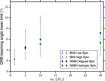
Figure 8. Lower limit on the beaming angle of short GRBs, as a function of the mass of the primary BH or NS, m1. We take the appropriate 90% rate upper limit from this Letter, assume all short GRBs are produced by each case in turn, and assume all have the same beaming angle θj. The limit is calculated using an observed short GRB rate of  Gpc−3 yr−1, and the ranges shown on the plot reflect the uncertainty in this observed rate. For BNS, m2 comes from a Gaussian distribution centered on 1.35 M⊙, and for NSBH, it is fixed to 1.4 M⊙.
Download figure:
Standard image High-resolution image7. CONCLUSION
We report the non-detection of BNS and NSBH mergers in advanced LIGO's first observing run. Given the sensitive volume of Advanced LIGO to such systems we are able to place 90% confidence upper limits on the rates of BNS and NSBH mergers, improving upon limits obtained from initial LIGO and initial Virgo by roughly an order of magnitude. Specifically we constrain the merger rate of BNS systems with component masses of 1.35 ± 0.13 M⊙ to be less than 12,600 Gpc−3 yr−1. We also constrain the rate of NSBH systems with NS masses of 1.4 M⊙ and BH masses of at least 5 M⊙ to be less than 3210 Gpc−3 yr−1 if one considers a population where the component spins are (anti-)aligned with the orbit, and less than 3600 Gpc−3 yr−1 if one considers an isotropic distribution of component spin directions.
We compare these upper limits with existing astrophysical rate models and find that the current upper limits are in conflict with only the most optimistic models of the merger rate. However, we expect that during the next two observing runs, O2 and O3, we will either make observations of BNS and NSBH mergers or start placing significant constraints on current astrophysical rates. Finally, we have explored the implications of this non-detection on the beaming angle of short GRBs. We find that if one assumes that all GRBs are produced by BNS mergers, then the opening angle of gamma-ray radiation must be larger than  , or larger than
  if one assumes all GRBs are produced by NSBH mergers.
The authors gratefully acknowledge the support of the United States National Science Foundation (NSF) for the construction and operation of the LIGO Laboratory and Advanced LIGO as well as the Science and Technology Facilities Council (STFC) of the United Kingdom, the Max-Planck-Society (MPS), and the State of Niedersachsen/Germany for support of the construction of Advanced LIGO and construction and operation of the GEO600 detector. Additional support for Advanced LIGO was provided by the Australian Research Council. The authors gratefully acknowledge the Italian Istituto Nazionale di Fisica Nucleare (INFN), the French Centre National de la Recherche Scientifique (CNRS) and the Foundation for Fundamental Research on Matter supported by the Netherlands Organisation for Scientific Research, for the construction and operation of the Virgo detector and the creation and support of the EGO consortium. The authors also gratefully acknowledge research support from these agencies as well as by the Council of Scientific and Industrial Research of India, Department of Science and Technology, India, Science & Engineering Research Board (SERB), India, Ministry of Human Resource Development, India, the Spanish Ministerio de Economía y Competitividad, the Conselleria d'Economia i Competitivitat and Conselleria d'Educació Cultura i Universitats of the Govern de les Illes Balears, the National Science Centre of Poland, the European Commission, the Royal Society, the Scottish Funding Council, the Scottish Universities Physics Alliance, the Hungarian Scientific Research Fund (OTKA), the Lyon Institute of Origins (LIO), the National Research Foundation of Korea, Industry Canada and the Province of Ontario through the Ministry of Economic Development and Innovation, the Natural Science and Engineering Research Council Canada, Canadian Institute for Advanced Research, the Brazilian Ministry of Science, Technology, and Innovation, Fundação de Amparo à Pesquisa do Estado de São Paulo (FAPESP), Russian Foundation for Basic Research, the Leverhulme Trust, the Research Corporation, Ministry of Science and Technology (MOST), Taiwan and the Kavli Foundation. The authors gratefully acknowledge the support of the NSF, STFC, MPS, INFN, CNRS, and the State of Niedersachsen/Germany for provision of computational resources.
Footnotes
- 141
Assuming a mass of 1.4 M⊙ and a moment of inertia = J/Ω of 1.5 × 1045 g cm2; the exact moment of inertia is dependent on the unknown NS equation of state (Lattimer 2012).
- 142
Calculated with a pulsar mass of 1.37 M⊙ and a high moment of inertia, 2 × 1045 g cm2.
- 143
This assumes an isotropic distribution of spins on both bodies. The systems that are not recovered well using search space where the dimensionless aligned spins are <0.05 are those systems where both spins are large, are aligned with the orbital plane, and point in the same direction. Such systems are quite rare when considering an isotropic distribution of spins.
- 144
The "chirp mass" is the combination of the two component masses that LIGO is most sensitive to, given by
 , where mi denotes the two component masses.
 - 145
The internal lalsimulation names for the waveforms used as filters described in this work are "TaylorF2" for the frequency-domain, post-Newtonian approximant, "SpinTaylorT4" for the time-domain approximant used by mbta, and "SEOBNRv2_ROM_DoubleSpin" for the aligned-spin effective-one-body waveform. In addition, for calculation of rate estimates describe in Section 5, the "SpinTaylorT4" model is used to simulate BNS signals and "SEOBNRv3" is used to simulate NSBH signals.
