


Abstract
EUV observations of a multi-thermal coronal loop, taken by the Atmospheric Imaging Assembly of the Solar Dynamics Observatory, which exhibits decay-less kink oscillations are presented. The data cube of the quiet-Sun coronal loop was passed through a motion magnification algorithm to accentuate transverse oscillations. Time–distance maps are made from multiple slits evenly spaced along the loop axis and oriented orthogonal to the loop axis. Displacements of the intensity peak are tracked to generate time series of the loop displacement. Fourier analysis on the time series shows the presence of two periods within the loop:  minutes and
  minutes. The longer period component is greatest in amplitude at the apex and remains in phase throughout the loop length. The shorter period component is strongest further down from the apex on both legs and displays an anti-phase behavior between the two loop legs. We interpret these results as the coexistence of the fundamental and second harmonics of the standing kink mode within the loop in the decay-less oscillation regime. An illustration of seismological application using the ratio P1/2P2 ∼ 0.7 to estimate the density scale height is presented. The existence of multiple harmonics has implications for understanding the driving and damping mechanisms for decay-less oscillations and adds credence to their interpretation as standing kink mode oscillations.
Export citation and abstract BibTeX RIS
1. Introduction
Plasma structures in the solar atmosphere are observed to act as waveguides for magnetohydrodynamical (MHD) waves, which can be related back to the medium's local plasma parameters through seismology (for comprehensive reviews of MHD oscillations see Aschwanden 2009; Nakariakov et al. 2016b and references therein). One intensively studied form of MHD wave is observed as transverse plane-of-sky displacements of plasma non-uniformities, interpreted as fast magnetoacoustic kink oscillations. Typically imaged in the EUV band, kink oscillations have been observed in coronal loops since the advent of the Transition Region And Coronal Explorer (TRACE; Aschwanden et al. 1999; Nakariakov et al. 1999) and more recently with the Atmospheric Imaging Assembly (AIA) on board the Solar Dynamics Observatory (SDO; Lemen et al. 2012; see Aschwanden & Schrijver 2011). The typical kink oscillation period Pkink is several minutes (see the statistical study by Goddard et al. 2016). As the period is determined by the loop length, the plasma densities inside and outside the loop, and the magnetic field, observations of kink oscillations allow for the seismological estimation of the (local) magnetic field, which is often difficult to determine directly (Liu & Ofman 2014). For a standing kink oscillation sustained in a coronal loop of length L, the period is related to the (averaged) kink speed CK through Pkink = 2L/CK.
If multiple, parallel harmonics of a standing mode are detected, it is possible to use the ratio of their periods as a seismological tool too. This was first demonstrated in Andries et al. (2005) using observations of higher harmonics in a loop arcade by TRACE, reported in Verwichte et al. (2004). The ratio of fundamental period P1 to twice the period of the second harmonic P2, succinctly P1/2P2, was used to probe the plasma structure by attributing any departure of this ratio from unity to the density stratification along the coronal loop. As was pointed out in Jain & Hindman (2012), the period ratio only contains information about the non-uniform distribution of the kink speed along the loop, and extra information is required to discriminate between density or field effects. Nevertheless, attributing this departure from unity to density stratification, several authors have derived analytical expressions for the dependence of P1/2P2 on density scale height H, including McEwan et al. (2008), Andries et al. (2005), Safari et al. (2007), and Ruderman & Petrukhin (2016). The model considered by Andries et al. (2005) and Safari et al. (2007) gives the following:
In De Moortel & Brady (2007), a harmonic was spatially resolved and anti-phase behavior between the legs on either side of the apex was observed, which is the expected behavior for an even harmonic, standing mode. More recently Pascoe et al. (2016) used AIA/SDO observations to spatially resolve the fundamental and second harmonic, justifying their interpretation by invoking the ratio of oscillation periods, the spatial dependence of the amplitudes for each mode, and anti-phase oscillations of the loop legs for the second harmonic. Seismological studies by Pascoe et al. (2017a, 2017b) found evidence of higher (second and/or third) harmonics in all cases of kink oscillations excited by external perturbations, consistent with the numerical simulations by Pascoe et al. (2009), but noticeably absent in the case of a kink oscillation generated by the post-flare implosion studied by Russell et al. (2015). In these and all previous cases of detection of multiple harmonics, the oscillation decayed rapidly.
Observations show that there are two regimes of kink oscillations. The first and most widely reported is large amplitude, rapidly decaying oscillations with displacements of the order of several loop minor radii and decay time of the order of several periods. In this regime, motions disappear completely after about 3.2 cycles on average (Goddard et al. 2016). The majority of these oscillations are excited by a mechanical displacement of the loop from equilibrium from an impulsive event such as a CME (Zimovets & Nakariakov 2015). The rapid decay is attributed to resonant absorption (e.g., Ruderman & Roberts 2002).
The second regime involves much lower amplitude oscillations that persist for far longer (over many periods) without disappearing, and in some cases grow over time (Wang et al. 2012). Anfinogentov et al. (2013) and Nisticò et al. (2014) observed decay-less oscillations independent of nearby eruptive events, implying their underlying driving mechanism is distinct and continuous. Nisticò et al. (2013) established that the decaying and decay-less regimes are able to coexist in the same loop, with decay-less oscillations detected before and after a large amplitude decaying oscillation triggered by an eruption. These persistent decay-less oscillations retained the same period throughout, equal to the period for the decaying oscillations, with far smaller amplitude (≈7% of the fundamental mode amplitude according to the seismological analysis by Pascoe et al. 2017a). A statistical study conducted in Anfinogentov et al. (2015) concluded that low-amplitude kink oscillations are omnipresent, being observed in 19 of 21 active regions investigated.
Due to the small amplitude of the decay-less oscillations, insufficient resolution of EUV imagers prevented their detection and measurement prior to 2012. One method to overcome this was developed and presented in Anfinogentov & Nakariakov (2016), where a motion magnification routine using a two-dimensional dual-tree complex wavelet transform enhanced transverse motions in the plane of sky. This technique uses both spatial and temporal information to reconstruct the image with magnified transverse oscillations over an unchanged stable background. The magnification is independent of oscillation period for a broad range of periods and scales linearly with the displacement amplitude, and thus makes a suitable tool to help clearly determine the oscillation parameters.
Until now, decay-less oscillations have only been seen with a single frequency per loop. Anfinogentov et al. (2015) demonstrated that the period of decay-less oscillations scales with loop length as in the decaying regime. However, their excitation mechanism is unknown and they are presumably subject to the same damping mechanisms as the decaying regime. Nakariakov et al. (2016a) suggested decay-less oscillations are the manifestation of a loop self-oscillation and outlined this model in a low-dimensional and semi-empirical manner citing the Rayleigh oscillator equation. This draws on an analogy of the loop as a violin string, with driving super-granulation flows near the loop footpoints acting as the violin bow. The period of the oscillation would then be determined by the loop parameters and not the driver, being consistent with the finding that no period was preferred to have higher amplitude, as would happen for a driven oscillator (Anfinogentov et al. 2015). This model naturally prescribes there should exist higher harmonics, similar to a violin note having overtones.
In this Letter, we report the first detection of multiple harmonics of decay-less kink oscillations in a coronal loop. Applying motion magnification to SDO/AIA observations of an off-limb coronal loop (Section 2), two strong periods are detected, with one period being approximately half the other. In Section 3, we present evidence from the the spatial distribution and phase distribution of the two periods to support our interpretation of the existence of the fundamental and second harmonic in the decay-less regime. We discuss the seismological implications of the detection of multiple decay-less harmonics in Section 4.
2. Observations
The coronal loop of interest is not associated with any active region and appeared on the (south westerly) limb of the Sun on 2013 January 21. It remained visible in 171 Å for approximately 10 hours. The loop is also visible in 193 Å and 211 Å channels. The loop is approximately semi-circular (Nisticò et al. 2014) and using this approximation its length was estimated as L ≈ 292 Mm. The loop appears as a bundle of multiple threads, with lifetimes of approximately 30–60 minutes. During the observation time, the loop length remains constant and no flares or eruptions were detected. In contrast to flare-induced large amplitude oscillations, low-amplitude oscillatory behavior was seen throughout the loop's existence, observed as transverse motions of individual threads.
For the detailed study, a time interval of 30 minutes (150 frames) was chosen, starting from 21:15:00 UTC. In this interval, one of the loop threads was best contrasted, including its legs, which was necessary for our analysis. A subfield of 1024 × 1024 pixels was extracted representing the region of interest. Since the loop extends beyond the limb, derotation was not required, therefore avoiding the potential introduction of artificial periodicities from interpolation artifacts.
The (projected) loop axis was fitted with a segment of an ellipse, and 100 straight slits with a length of 100 pixels were created perpendicular to this axis at equal increments along the loop's axis (see Figure 1). By analyzing the oscillation signal in many locations, a good precision may be obtained in a similar manner to Van Doorsselaere et al. (2007), and for this well-contrasted loop segment the spatial distribution of any harmonics is resolvable. Time–distance maps are made from these slits, and for each slit the intensity is averaged over a width of five pixels in order to improve the signal-to-noise ratio. Only in slits 35–85 was the loop contrasted well enough to be used reliably in further analysis, due to the presence of the limb and time-varying noise from the lower corona. The motion magnification also suffers distortion from motions in the background, making slits nearby unusable at the relatively active limb. The length of loop segment between consecutive slit index numbers varies slightly along the loop due to loop curvature and projection. However, this dependence is small since the loop plane is reasonably perpendicular to the observer, and the loop is approximately semi-circular. So, its curvature is approximately constant along the loop.

Figure 1. SDO/AIA 171 Å image of the loop at data start time 2013 January 21 21:15:00 UT. Note that this intensity image has been enhanced using the Multiscale Gaussian Normalization (Morgan & Druckmüller 2014). Slits that were used for the analysis are displayed, taken perpendicular to an elliptical fitting of the loop, whose footpoints are shown by the black crosses.
Download figure:
Standard image High-resolution imageThe data cube was passed through the motion magnification algorithm (Anfinogentov & Nakariakov 2016) with a magnification factor of 6. Testing not included here showed the data were robust to different routine parameters, and the oscillation is visible in the data before magnification.
3. Results
3.1. Spectral Analysis
Each of the 50 slit's time–distance maps underwent an intensity fitting procedure at each frame, creating a time series that follows the highest intensity peak through time that is assumed to be the position of the loop axis in a similar manner to that described in Pascoe et al. (2016). Fourier analysis was performed to obtain the power spectrum of each time series. Figure 2 shows these spectra stacked to form a two-dimensional distribution of (normalized) spectral power as a function of period and distance along the loop (the slit index). Three regions of significant spectral power are visible. The strongest signal is seen for slit numbers ∼63, which is near the loop apex, with a period of  minutes. This value was measured by summing the Fourier power spectra for the slits with spectral power above a threshold value (in this case slits 60–68) and extracting the period value corresponding to this sum's peak. The error is estimated as the FWHM, for this slightly asymmetric peak. For slit numbers ∼74, corresponding to the southern loop leg, there is significant spectral power with a period of
  minutes. This period and FWHM was measured through summing spectra from slits 70 to 78. A similar region of significant power is seen for slit numbers ∼43 corresponding to the northern loop leg, with a period of
  minutes. This value was measured from the summation of spectra from slits 40–48.
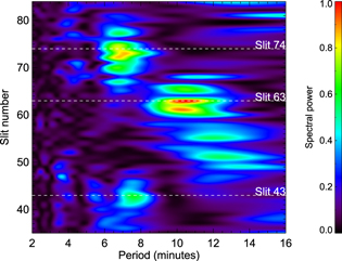
Figure 2. Two-dimensional distribution of Fourier spectral power per slit against period and slit number.
Download figure:
Standard image High-resolution imageThese results are interpreted as the fundamental and second harmonic of the standing kink mode for the following reasons. First, there are two distinct periods, one being approximately half of the other. The longer period of ∼11 minutes lies within the range expected for the fundamental standing kink mode for a loop of this size, i.e., CK ≈ 0.9 Mm s−1. The shorter period component lies at slightly greater than half of this value at ∼7.4 minutes, with both regions being measured as the same period within error. This period is consistent with a second harmonic modified by effects such as density stratification. The spatial distribution of the nodes and anti-nodes for the two periodicities (Figure 2) is also consistent with the fundamental and second harmonic standing modes.
3.2. Fitting Frequency and Phase
Figure 3 compares time–distance maps from slits 43 (northern leg), 63 (near apex), and 74 (southern leg). Each map is overplotted with the fitted intensity time series in black and a sinusoid that has been fitted to the time series in blue. By comparing the top and bottom plots, one can see that the periods of fitted sinusoids are similar (7.8 and 7.0 minutes, respectively) and the oscillations are approximately in anti-phase as expected for two anti-nodes of the second harmonic. The time–distance map for slit 63 exhibits a much longer period of 10.3 minutes.

Figure 3. Time–distance maps for slits 43 (bottom), 63 (middle), and 74 (top). The solid blue line shows the time series output from the time–distance map intensity fitting. The dashed black line is the least squares fit of the time series to a single sinusoid. Thus, for slit 43 (bottom), the dashed black line is a sinusoid of period 7.8 minutes, amplitude 0.62 Mm, and phase 128°. For slit 63 (middle), the dashed black line is a sinusoid of period 10.3 minutes, amplitude 0.93 Mm, and phase 33°. For slit 74 (top), the dashed black line is thus a sinusoid with fitted period of oscillation of 7.0 minutes, amplitude 1.4 Mm, and phase 20°.
Download figure:
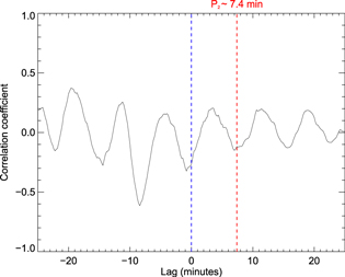
Standard image High-resolution imageFurther evidence that the higher-frequency component is an even harmonic comes from Figure 4, which clearly shows the existence of the same frequency component in both slits 74 and 43, i.e., on opposite legs as expected. The value at lag zero (blue dashed line) is negative and has a local minimum, meaning the two legs are in anti-phase, as expected for an even harmonic. The oscillation is apparent for all lags without significant decay of amplitude, especially considering that for greater lags there is less signal to contribute to the cross-correlation, showing the oscillation is decay-less.
Figure 4. Cross-correlation between slits 43 and 74 as a function of lag. The dotted blue line at lag 0 intersects the cross-correlation at the Pearson coefficient value. The dotted red line at lag 7.4 minutes is displayed to show the period of the higher-frequency component P2 calculated from the Fourier analysis (interval between the red and blue lines). The cross-correlation is oscillatory with this period.
Download figure:
Standard image High-resolution image
4. Discussion
In this Letter, data from a well-contrasted loop extending off-limb, observed on 2013 January 21 with SDO/AIA, were processed using motion magnification (Anfinogentov & Nakariakov 2016). Fifty time–distance maps were created along the loop, and time series that follow the intensity peak (loop axis) were formed. Spectral analysis found two periods to be prominent. The longer period was found to be  minutes and the shorter period
  minutes. The spatial distribution of spectral amplitude revealed the shorter period component had an anti-node on each loop leg, and the longer component had an anti-node near the apex of the loop. Direct comparison of the time–distance maps and the cross-correlation analysis showed that the shorter period oscillations observed in different legs of the loop are in anti-phase. Taking into account the ratio of periods, the spatial distribution of spectral power into nodes and anti-nodes throughout the loop, and anti-phase behavior between the two legs, this observation provides good evidence for the existence of multiple harmonics within the decay-less regime. The existence of a spatial distribution of spectral power, partitioning the loop between equidistant anti-nodes, also provides evidence that decay-less oscillations are the result of standing kink mode, which is already strongly suggested by the period ranges and scaling with loop length (Anfinogentov et al. 2015).
Decay-less oscillations have several seismological applications. In addition to estimating the local Alfvén speed CA0 from the (fundamental) kink mode period, if a higher-order harmonic of the decay-less standing kink mode is also detected, then it is reasonable to assume that the density stratification affects the P1/2P2 ratio as it does in the decaying regime. Assuming that Equation (1) is valid for this data, the period ratio can provide an estimate for the density scale height (Andries et al. 2005; Safari et al. 2007). In this case, we estimate the P1/2P2 ratio as 10.3/(7.1 + 7.7) ≈ 0.69 ± 0.16, which for a loop with a length of L = 292 Mm yields a density scale height of H approximately in the range 7–45 Mm. This is less than the expected hydrostatic value, while it is consistent with the value of  Mm reported in Van Doorsselaere et al. (2007) and the value of 18–42 Mm reported in Pascoe et al. (2017a). We need to stress that any departure from unity of the P1/2P2 ratio is due to the non-uniform distribution of the kink speed along the loop, and more information is required to establish the mechanism that has changed the kink speed (Jain & Hindman 2012). Our estimation was made under the assumption that the kink speed variation was caused by the density stratification only. However, other effects may be important such as cross-section (magnetic) variation (e.g., Verth & Erdélyi 2008; Pascoe & Nakariakov 2016), temperature difference effects (e.g., Guo et al. 2015; Lopin & Nagorny 2017), siphon flows (e.g., Yu et al. 2016), and ellipticity of the loop (Dymova & Ruderman 2006). For more information on these effects, the reader is referred to the review in Andries et al. (2009). Here, the estimation is presented as an illustration of seismological application rather than detailed analysis of the precise value, which should be the subject of a dedicated study.
The finding that there exist multiple, spatially resolved harmonics within the decay-less regime provides evidence that these are the same kink mode standing waves as the large amplitude decaying regime; however, the precise origins of the decay-less oscillations remains poorly understood. The self-oscillation model outlined in Nakariakov et al. (2016a) fits with the results for decay-less oscillations found in Anfinogentov et al. (2015), including the range of period values, since the period is determined by the fundamental kink mode for that loop, and linear dependence of period on loop length. Higher harmonics, which are now known to exist, would naturally appear in the self-oscillation model; however, the development of at least a 1D model of kink self-oscillations is required to explicitly show this. Either way the result presented here constrains models of decay-less oscillations to include provision for higher harmonics, which remain stationary over many oscillation cycles.
The omnipresence of decay-less oscillations of coronal loops (Anfinogentov et al. 2015) suggests that the detection of the higher-order harmonics allows for the routine application of seismological techniques based on the P1/2P2 ratio to potentially all coronal loops, as observers would not need to rely on difficult to predict explosive events to act as a trigger as they do for large amplitude decaying oscillations. Seismology using decay-less oscillations may be used to constrain magnetic field extrapolations and additionally, if it can be found, using the P1/2P2 ratio to disentangle magnetic structure and density stratification.
This study was supported by the British Council Institutional Links Programme (the "Seismology of Solar Coronal Active Regions" project). V.M.N. acknowledges the support of the BK21 plus program through the National Research Foundation funded by the Ministry of Education of Korea. T.D. acknowledges the support of the UK STFC PhD studentship.
Software: Motion magnification (Anfinogentov & Nakariakov 2016; https://github.com/Sergey-Anfinogentov/motion_magnification).