


Abstract
Bowman et al. reported low-frequency photometric variability in 164 O- and B-type stars observed with K2 and TESS. They interpret these motions as internal gravity waves, which could be excited stochastically by convection in the cores of these stars. The detection of internal gravity waves in massive stars would help distinguish between massive stars with convective or radiative cores, determine core size, and would provide important constraints on massive star structure and evolution. In this work, we study the observational signature of internal gravity waves generated by core convection. We calculate the wave transfer function, which links the internal gravity wave amplitude at the base of the radiative zone to the surface luminosity variation. This transfer function varies by many orders of magnitude for frequencies ≲1 days−1, and has regularly spaced peaks near 1 days−1 due to standing modes. This is inconsistent with the observed spectra that have smooth "red noise" profiles, without the predicted regularly spaced peaks. The wave transfer function is only meaningful if the waves stay predominately linear. We next show that this is the case: low-frequency traveling waves do not break unless their luminosity exceeds the radiative luminosity of the star; the observed luminosity fluctuations at high frequencies are so small that standing modes would be stable to nonlinear instability. These simple calculations suggest that the observed low-frequency photometric variability in massive stars is not due to internal gravity waves generated in the core of these stars. We finish with a discussion of (sub)surface convection that produces low-frequency variability in low-mass stars; this is very similar to that observed in Bowman et al. in higher-mass stars.
Export citation and abstract BibTeX RIS
1. Introduction
Massive stars play an important role in astrophysics, driving galactic turbulence that regulates star formation (Hayward & Hopkins 2016) and enriching the chemical composition of the interstellar medium (Nomoto et al. 2013). It is thus important to test and calibrate models of massive star structure and evolution. Asteroseismology is an unparalleled technique to probe the interiors of stars (Aerts et al. 2010), and space-based photometry has revolutionized our understanding of stellar interiors (e.g., Aerts et al. 2019).
The detection of internal gravity waves, which propagate to the bottom of a star's radiative zone, provides precious information about the cores and interiors of massive stars (e.g., Zwintz et al. 2017; Ouazzani et al. 2019). Bowman et al. (2019b, hereafter B19) detected low-frequency variability in a large population of massive stars (following similar detections in fewer stars by, e.g., Blomme et al. 2011). In over 100 massive stars, B19 detected luminosity variations with roughly constant amplitude for frequencies ≲1 days−1, and power laws with slope −2 to −3 at higher frequencies. This "red noise" signal is very different from previous detections of discrete peaks in the power spectrum, which is likely due to linearly unstable g-modes (Pápics et al. 2017). B19 interpret this low-frequency variability as internal gravity waves, which could be excited by core convection.
Much of the early work on wave generation by convection was motivated by the Sun and stars with convective envelopes (e.g., Press 1981; Goldreich & Kumar 1990). These theories were extended to massive stars with convective cores (e.g., Lecoanet & Quataert 2013), and were validated by high-resolution, turbulent, 3D numerical simulations in Cartesian geometry (Couston et al. 2018). They find an excitation spectrum that decreases rapidly for frequencies above the convective turnover frequency. In contrast, work by other authors has found extremely shallow wave spectra at high frequencies (Rogers et al. 2013; Edelmann et al. 2019). There is currently no consensus on the spectrum of internal gravity waves at the radiative–convective boundary.
Simulations of wave excitation by convection do not follow the propagation of internal waves to the surface. To predict surface luminosity fluctuations, Samadi et al. (2010) and Shiode et al. (2013) solved the wave propagation problem using eigenmodes and the Wentzel–Kramers–Brillouin (WKB) approximation, but only considered standing modes. These calculation cannot predict the wave amplitude at frequencies between or below the frequencies of the standing modes. Thus, they do not replicate the "red noise" signal observed in B19. Here we test whether or not the signal can be explained by traveling waves; there is no previous work studying the surface manifestation of traveling waves in massive stars.
2. Internal Gravity Wave Propagation
The luminosity variations at the surface of a star δL(f; R⋆) are related to the radial velocity variations at the radiative–convective boundary  by
by

for linear waves. Here f is the frequency of the wave, and T(f) is the wave transfer function. We check the linearity assumption in Section 3. Equation (1) separates out the nonlinear physics related to convection, which determines  and is uncertain, from the linear physics of wave propagation, which gives T(f).
We will discuss the wave transfer function for a 10 M⊙, solar-metallicity star near the zero-age main sequence (ZAMS). The stellar structure model is calculated using MESA (Paxton et al. 2011, 2013, 2015, 2018, 2019). Appendix G shows the wave transfer function for stars from 3 M⊙ to 20 M⊙, and from the ZAMS to the terminal-age main sequence (TAMS). The broad features of the transfer functions are similar in this range of masses and ages.
We calculate the wave transfer function in two ways. First, we use non-adiabatic eigenmodes calculated with GYRE (Townsend et al. 2018). We assume the non-adiabatic eigenmodes form a complete basis, and expand the perturbations in this basis. We force the horizontal displacement with  at a forcing radius rf above the radiative–convective boundary. This produces a luminosity variation at the surface L(R⋆) with frequency f. We then calculate L(R⋆) for multiple forcing radii in a 0.02R⋆ range above the radiative–convective boundary. We force at multiple radii to avoid the nodes of the eigenfunctions. T(f) is the average of the amplitude of L(R⋆) over these forcing radii.
To validate this calculation, we also time-evolve the linearized non-adiabatic oscillation equations in the Cowling approximation (Equations (33)–(39)) using Dedalus (Burns et al. 2019). We solve the equations from the radiative–convective boundary (rRCB ≈ 0.22R⋆) to the bottom of the surface convection zone (rtop ≈ 0.98R⋆). We cannot include the core or surface convection zones in the simulation; otherwise, linearly unstable convective modes dominate. We force the waves with a boundary condition  . After an initial transient, the luminosity at the top of the domain,
  , also varies sinusoidally, which allows us to measure T(f). We find good agreement between these two methods of calculating the wave transfer function. Appendices A–F include more details of the calculations, as well as the comparison between them.
Figure 1 shows the wave transfer function calculated using GYRE for spherical harmonic degrees ℓ = 1, 2, and 3. The ℓ = 1 mode dominates the surface luminosity fluctuations (Figure 2). For each ℓ, we see the transfer function is smooth at low frequencies, as is observed. However, the transfer function is also very small due to strong wave damping at low frequencies. If the observed low-frequency variability is due to waves from the core, there should be very little power for f ≲ 0.1 days−1, because these waves are strongly damped. The observed luminosity fluctuations are roughly constant even for f ≲ 0.1 days−1 (Figure 2 and Blomme et al. 2011). However, it is likely the low-frequency observations are dominated by systematic errors, so this inconsistency at low frequencies does not rule out the detection of propagating internal gravity waves at higher frequencies.
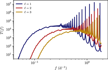
Figure 1. Wave transfer function T(f) for a 10 M⊙ star near the ZAMS. The transfer function has units of L/L⋆ per  . The transfer function is very small at low frequencies due to radiative damping. At higher frequencies near 1 days−1, the transfer function is dominated by sharp peaks associated with standing g-modes.
Download figure:
Standard image High-resolution image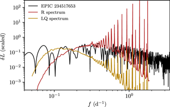
Figure 2. Luminosity variation spectrum for EPIC 234517653 from B19, and two theoretical spectra with different assumptions for the convective excitation spectrum,  . Because the theoretical spectra are for linear waves, their overall amplitude is arbitrary. The theoretical spectra show a sharp decline in wave amplitude for waves with f ≲ 0.1 day−1. They also show regularly spaced peaks at higher frequencies, f ≳ 1 day−1. Neither of these features are in the observed spectrum.
Download figure:
Standard image High-resolution imageFigure 1 also shows large-amplitude, regularly spaced peaks at frequencies ≳1 day−1. The peaks are at the frequencies of standing g-modes. These frequencies are the resonant frequencies for propagating internal gravity waves. Peaks with this type of regular spacing are not present in the observed data. Thus, we believe the observed low-frequency variability in high-mass stars is not due to linearly propagating internal gravity waves generated in the core.
Because the observed power spectra do not have regularly spaced peaks, one may be tempted to attribute the low-frequency variability to propagating, rather than standing, internal gravity waves. However, propagating internal gravity waves only produce a smooth spectrum when the damping rate is similar or greater than the mode frequency spacing. This is only true for waves that are strongly damped, which are too low amplitude to be observed. This dichotomy is illustrated by the wave transfer functions in Figure 1: the transfer function is smooth for low frequencies, but is also very small; whereas at higher frequencies it is dominated by large-amplitude peaks.
To illustrate this point, in Figure 2 we compare the observed spectrum of EPIC 234517653 from B19 to two theoretical spectra. We choose this star because it has spectral type B2, roughly corresponding to our 10 M⊙ stellar model, and has a relatively simple spectrum without strong rotation effects or signature of linearly unstable modes. Although we plot the "residual" spectrum, the "original" spectrum is qualitatively similar.
The theoretical spectrum depends on the wave excitation spectrum  via Equation (1). To show a range of possibilities, we consider two very different excitation spectra reported in numerical simulations. Rogers et al. (2013) ran a series of 2D cylindrical simulations using the anelastic equations, and found
  , where
  (Ratnasingam et al. 2019); we refer to results using this spectrum with R. Couston et al. (2018) ran a series of 3D cartesian simulations using the Boussinesq equations, and found
  we refer to results using this spectrum with LQ, as they match with the theoretical prediction in Lecoanet & Quataert (2013). We then sum luminosity variations over ℓ using the Dziembowski (1977) relations as in Shiode et al. (2013). To maintain the same frequency resolution as the observations, we calculate the maximum brightness fluctuation in frequency bins with the same width as the frequency spacing of the observational data from B19.
Figure 2 shows the luminosity variation spectrum for EPIC 234517653, as well as the R and LQ spectra. The overall normalization of the theoretical spectra are scaled to more easily compare to the observations. The predicted normalization of the LQ spectrum is similar what we plot, whereas the predicted normalization of the R spectrum is about 4 orders of magnitude higher than what we plot (Appendix H). The theoretical spectra inherit two important properties from the wave transfer function (Figure 1): (1) at low frequencies (f ≲ 0.1 days−1), the luminosity perturbations become very small due to strong wave damping; and (2) at frequencies ≳0.5 day−1, there are regularly spaced peaks due to the near-resonant effects of standing modes. Neither of these features are in the observations, which show a fairly flat spectrum at low frequencies, without regularly spaced peaks at higher frequencies. Our calculations do not take into account rotation. Rotation would increase the number of resonant peaks at high frequencies, but also decrease the luminosity variation at low frequencies. Appendix I shows that the high-frequency waves would still manifest as a series of resonant peaks, so rotation does not change the main features of Figure 2.
Although here we only compare to a single star, none of the spectra in B19 show a large number of regularly spaced peaks similar to the theoretical spectra in Figure 2. Even stellar power spectra that do have peaks (e.g., EPIC 202061164) only have a couple, and thus do not match the theoretical spectra for convectively excited internal gravity waves. The standing waves in the R spectrum reach very large amplitudes, which would probably lead to nonlinear interactions. However, in the next section we show that the observed variability is too small to be nonlinear.
3. Internal Gravity Wave Nonlinearity
In the previous section, we showed that linearly propagating waves have a surface luminosity spectrum inconsistent with observations. Here we will investigate possible nonlinear effects. We argue that traveling waves do not become strongly nonlinear, i.e., break. While standing waves could in principle experience weak nonlinearities, we show that the observed luminosity fluctuations are so low that an equivalent standing wave would be stable to nonlinear instabilities. Thus, all the peaks of the predicted spectrum should be observable.
3.1. Traveling Wave Breaking
In the absence of damping, waves conserve the wave luminosity as they propagate outward,

Here ξh is the horizontal wave displacement, ω is the wave's angular frequency, N is the Brunt–Väisälä frequency, and  and kr are the horizontal and radial components of the wavenumber. In deriving Equation (2) we have approximated the dispersion relation as
  .
.
As waves propagate outward, ρ decreases, leading ξh to increase. When ξh kh ∼ 1, waves break quickly in about a wave period (e.g., Staquet & Sommeria 2002; Liu et al. 2010; Eberly & Sutherland 2014). Thus, the criterion for wave breaking is

The total wave luminosity is expected to be smaller than the convective luminosity by a factor of the convective Mach number (e.g., Goldreich & Kumar 1990; Lecoanet & Quataert 2013); this scaling was verified in the simulations of Rogers et al. (2013) and Couston et al. (2018).
Radiative damping is significant for some waves. Waves are weakly affected by damping if they propagate further than one pressure scaleheight H over a damping time,

where Krad is the radiative diffusivity. This is a conservative estimate: waves need to propagate many scaleheights for them to reach the surface without damping. We can rewrite this in terms of the radiative luminosity using  . Then a requirement for waves to not experience significant damping is

If waves are radiatively damped, they will not reach sufficient amplitudes to break. So combining this with Equation (3), we find a requirement for waves to break is

Since the wave luminosity is significantly smaller than the convective luminosity, this relation is not satisfied in almost all stars (some stars in the last year of their life may have  ; see Quataert & Shiode 2012). Thus, traveling waves will not experience wave breaking. Note, however, that many numerical simulations artificially increase the convective luminosity by many orders of magnitude (e.g., Rogers et al. 2013; Jones et al. 2017; Edelmann et al. 2019), which likely explains reports of breaking waves generated by convection in Rogers et al. (2013) and Edelmann et al. (2019). Artificially increasing the convective (and hence wave) luminosity makes it difficult to study wave excitation and propagation, because the wave physics can be very different.
3.2. Nonlinear Stability of Standing Waves
Figure 1 shows that waves excited near the star's g-mode frequencies can experience resonant amplification. Because the resonant waves are coherent for many wave periods, weakly nonlinear effects can build up over time, and lead to significant transfer of energy between frequencies without necessitating wave breaking.
However, the observed luminosity fluctuations are very small. Even if the entire luminosity variation was due to standing modes, the modes would be stable to nonlinear instability for most low-ℓ standing modes in 10 M⊙ ZAMS stars. As discussed in Weinberg et al. (2012), nonlinear instabilities of a "parent" mode with frequency f and amplitude ξh kh requires the existence of two other modes satisfying
where κ is a spatial overlap integral, γ1 and γ2 are the damping rates of the two "daughter" modes, and δf is the frequency difference between the parent and daughter modes, all measured in units of day−1. The difference between the ℓ of the daughter modes can be no greater than the ℓ of the parent mode.
We calculate the threshold for nonlinear instability by finding the smallest possible ξh kh satisfying Equation (7) for each mode. We search over modes with ℓ ≤ 20 with daughter mode frequencies less than the parent mode frequency so they can efficiently damp. We assume that the spatial overlap integral κ is small if the difference between the radial mode orders is greater than two; otherwise we take κ = 1. In Figure 3, we plot the surface luminosity fluctuations associated with these marginally stable modes. All but one ℓ = 1 mode would be nonlinearly stable, even if we assume the observed fluctuations are entirely due to those modes. We also find nonlinear stability for modes with f ≤ 1 day−1.

Figure 3. Stability threshold of weakly nonlinear standing waves in comparison to the observed spectrum for EPIC 234517653 from B19. The symbols show the luminosity variation of a marginally stable standing mode of a given ℓ. Most modes require greater-than-observed luminosity variations to be unstable to weakly nonlinear instabilities.
Download figure:
Standard image High-resolution imageLess-massive and more evolved stars have more weakly damped modes, so some standing modes experience nonlinear instabilities in these stars. We also note that some stars in B19 show several peaks, likely due to linearly unstable g-modes. In many cases, those peaks are at amplitudes that are similar to the marginally stable amplitude calculated in Figure 3. Many other stars show signatures of nonlinear wave interaction (e.g., Degroote et al. 2009; Bowman et al. 2016). In pulsating white dwarfs (ZZ Ceti stars), the mode amplitudes are also believed to be limited by weak nonlinearities (e.g., Wu & Goldreich 2001; Luan & Goldreich 2018). However, in none of these cases is there any indication that these interactions can produce the "red noise" spectra observed in B19.
4. Subsurface Convection
We have argued that the observed low-frequency variability is massive stars is unlikely due to internal gravity waves generated by core convection. Another possible source of the variability is surface phenomena.
Stars with spectral types later than F have well-developed surface convection zones driven by hydrogen ionization. In these stars, turbulent convection results in a specific photometric signature: granulation. In the power spectrum, granulation shows up as an excess of power at low frequencies (red noise). 3D radiative hydrodynamical simulations of surface convection can match observations of the disk-integrated intensity of main-sequence stars and red giants (e.g., Samadi et al. 2013a, 2013b, and references therein). Convective surface velocity fluctuations also affect stellar spectra. If the surface velocity fluctuations are correlated over the entire line-forming region, this is referred to as macroturbulence. Otherwise it is referred to as microturbulence.
Both micro- and macro- turbulence have also been observed in OB stars, with amplitudes ranging from a few to tens of km s−1. These stars are not convective at the surface, but possess subsurface convective layers due to partial ionization of helium and iron group elements (Cantiello et al. 2009; Cantiello & Braithwaite 2019). Cantiello et al. (2009) and Grassitelli et al. (2015a, 2015b) show that the presence and vigor of subsurface convection is correlated to spectroscopically derived surface velocity fluctuations in OB stars. This is true for all stars except those with magnetic fields strong enough to substantially affect the iron subsurface convection zone (Sundqvist et al. 2013). This suggests that subsurface convection could play an important role in inducing stellar surface variability, even for OB stars.12
It is thus natural to ask if the observed low-frequency variability in massive stars is also caused by subsurface convection. This was discussed in Bowman et al. (2019a), which showed that the variability in massive stars has a characteristic frequency νchar of a few tens of μHz, with little dependency on the star's position on the HR-diagram. This is inconsistent with the "KB-scaling" of convective frequency with stellar properties derived in Kjeldsen & Bedding (1995) (see Figure 8 in B19).
However, Kjeldsen & Bedding (1995) derived this scaling for surface convection. The KB-scaling matches observations of stars with surface temperatures below approximately 10–11,000 K, which have surface convection driven by hydrogen and helium ionization. For hotter stars, convection occurs below the surface around temperatures corresponding to partial ionization of He ii (≈45 kK) and Fe (≈150 kK). These subsurface convective regions (He iiCZ and FeCZ) occur at the specified temperatures; if a star expands, they will move to deeper mass coordinate. As such, they do not directly trace stellar surface properties, and one does not expect their induced surface photometric fluctuations to follow the KB-scaling. Instead, models predict a fairly constant value of their characteristic frequency as function of the stellar parameters, with typical frequencies of 6–60 μHz (Cantiello et al. 2009; Cantiello & Braithwaite 2011, 2019), which are consistent with the range of characteristic frequencies observed in the Bowman et al. (2019a) sample. Hence, we argue the distribution of characteristic frequencies of the observed low-frequency variability may support a subsurface origin.
The low-frequency variability is also observed in low-metallicity Large Magellanic Cloud (LMC) stars (B19). Since the occurrence of the FeCZ is metallicity dependent, this could rule out subsurface convection as the cause of the variability. In 1D stellar evolution calculations, the FeCZ occurs above a luminosity of  for solar-metallicity stars, corresponding to a ZAMS star of about
  . At the lower metallicity of the LMC, the FeCZ appears at higher luminosities (L ≈ 103.9
  ), corresponding to a ZAMS star of about
  (Cantiello et al. 2009). However, it is unclear if the objects in the TESS LMC sample of B19 are hot, main-sequence stars probing this FeCZ transition luminosity. For example, if the sample contains mostly luminous giants and supergiants, then the stars could be either above the FeCZ luminosity threshold for LMC metallicity, or posses surface convection due to H and He ionization. This would also be consistent with the much larger amplitude of the photometric variability of the LMC sample, as expected in more massive, brighter stars, independent of the scenario considered (subsurface convection or core internal gravity waves).
Finally, some of the stars showing low-frequency, stochastic variability are low-mass, main-sequence A stars. These are not expected to show the presence of an FeCZ. However, they are affected by other (sub)surface convection zones due to the ionization of H and He (Cantiello & Braithwaite 2019). While the amplitude of the velocity fluctuations induced by these convective regions tend to be smaller than for the FeCZ, characteristic frequencies are also in the range of tens of μHz.
Therefore, subsurface convection remains a viable explanation for the observed variability. More work is required to test this hypothesis and firmly establish—or rule out—a connection between subsurface turbulent convective motions and the wide-spread, low-frequency photometric variability observed in massive stars.
5. Summary
- 1.We argue that the low-frequency variability presented in B19 is not due to linearly propagating waves from the core.
- i.At low frequencies, linear waves have a smooth spectrum, but very little surface luminosity variation due to strong radiative damping. This is not observed.
- ii.Linearly propagating waves at frequencies f ≳ 0.5 day−1 form many standing modes (Figure 2), which are also not observed.
- 2.Wave propagation can be approximated as linear.
- i.Low-frequency traveling waves do not break.
- ii.If high-frequency variability was due to standing modes, many would be at such low amplitude they would be stable to nonlinear interactions.
- 3.We conclude that the spectra presented in B19 are not due to IGWs generated by core convection.
- 4.However, almost all massive stars have subsurface convection zones that could produce the observed low-frequency variability.
We are grateful for extremely useful discussions with Conny Aerts, Dominic Bowman, and Siemen Burssens regarding the observations presented in B19. We would like to thank Rich Townsend for valuable discussions about GYRE and stellar oscillation modes. We would also like to thank Tamara Rogers, Rathish Ratnasingam, and Philipp Edelmann for useful conversations about wave nonlinearity. We would also like to thank the anonymous referee who pointed out some additional reasons why the observations of B19 are unlikely to be due to waves generated in the core. D.L. is supported by a PCTS and Lyman Spitzer Jr. fellowship. D.L. would like to thank his fellow members of the 10th New York County Grand Jury #6 of 2019 for their amiable company while he composed this paper during his four weeks of jury service. The Center for Computational Astrophysics at the Flatiron Institute is supported by the Simons Foundation. This work has benefited from many conversations at meetings supported by Grant GBMF5076 from the Gordon and Betty Moore Foundation. E.Q. thanks the Princeton Astrophysical Sciences department and the theoretical astrophysics group and Moore Distinguished Scholar program at Caltech for their hospitality and support. L.A.C. acknowledges funding from the European Union's Horizon 2020 research and innovation programme under the Marie Sklodowska-Curie grant agreement No. 793450. L.A.C., B.F., and M.L.B. acknowledge funding by the European Research Council under the European Union's Horizon 2020 research and innovation program through grant No. 681835-FLUDYCO-ERC-2015-CoG. This work was performed in part under contract with the Jet Propulsion Laboratory (JPL) funded by NASA through the Sagan Fellowship Program executed by the NASA Exoplanet Science Institute. B.J.S.P. acknowledges being on the traditional territory of the Lenape Nations and recognizes that Manhattan continues to be the home to many Algonkian peoples. We give blessings and thanks to the Lenape people and Lenape Nations in recognition that we are carrying out this work on their indigenous homelands.
Appendix A: Bulk Forcing of IGWs
We use the non-adiabatic g-mode oscillations of a star as a basis to expand velocity perturbations. For a given spherical harmonic degree ℓ, we have

where  corresponds to the velocity eigenfunction, and
  its (complex) frequency. For simplicity of notation, here we will write frequencies in terms of the angular frequency
  , and write velocity perturbations as
  , instead of
  as in the main text. The velocity eigenfunctions are related to the displacement eigenfunctions via
  . All vectors are assumed to be composed of two components: a radial component, e.g., ur; and a horizontal component which is assumed to be proportional to the horizontal gradient of a spherical harmonic function, e.g.,
  , where
  represents a horizontal angular derivative.
The eigenfunctions satisfy

where  is the linear wave operator. We define the dual basis
  by
by

where δ is the Kronecker delta function, and the inner product is defined as

We can define the dual basis in this way because the eigenvalues are non-degenerate. The set of all adiabatic modes are a complete basis (e.g., Eisenfeld 1969). Non-adiabatic modes are likely not complete (R. H. D. Townsend 2019, personal communication). Nevertheless, we expect they can represent almost all functions in the regions of the star that do not experience strong damping. The good agreement with calculations using Dedalus indicates the non-adiabatic modes can faithfully represent traveling waves.
We now introduce a forcing to the system,

The forcing has magnitude  , is assumed to act in only the horizontal directions, at the forcing radius rf, and at frequency ω,

where δ is the Dirac delta function. We can solve Equation (12) by using the expansion in normal modes (Equation (8)) and projecting out with  . This gives
Defining  and assuming ρ is a function of radius, we can simplify this to
This can be solved together with the boundary condition Aℓ = 0 at t = 0,
Substituting this into Equation (8), we find
If all the eigenmodes are damped, the imaginary part of  is negative. As
  , the second exponential term drops out, and we find
The surface luminosity fluctuations are then
where  is the surface luminosity perturbation of the mode with frequency
  . In practice, for many stellar models, we find that all modes calculated using GYRE are damped. Some stellar models do have some unstable modes with small positive growth rates. Nevertheless, we treat the time dependence of these modes in the same way as damped modes.
Appendix B: Connection between Bulk Forcing and Interface Forcing
Theories (e.g., Lecoanet & Quataert 2013) and simulations (e.g., Rogers et al. 2013) make predictions for how the radial velocity perturbations at the radiative–convective boundary depends on frequency and spherical harmonic degree,  . To use Equation (19), we need to establish a link between the radial velocity perturbations and the forcing amplitude
  .
.
To illustrate this connection, we will solve the bulk and interfacing forcing problems for an inviscid, adiabatic, Boussinesq fluid in Cartesian geometry. We assume the background has a constant Brunt–Väisälä frequency, N, ranges from z = 0 to L, that gravity is in the z direction, and that the perturbations are periodic in the horizontal directions. For impenetrable boundary conditions (uz(0) = uz(L) = 0), the eigenmodes are

where
The horizontal wavenumber kh is defined by  . The eigenvalues are frequencies ω which satisfy kz L = nπ, for an integer n.
Now consider the problem with boundary forcing. Our new boundary conditions are  , and uz(L) = 0. The solution to this new problem is
Recall that kz is a function of the forcing frequency (Equation (21)). One can verify that this satisfies the boundary conditions. We can calculate the amplitude of uz using
The amplitude diverges when kz L = n π, for n an integer. This corresponds to the frequencies of the eigenmodes of the system with impenetrable boundary conditions. Thus, the solution to the forced problem is related to the unforced eigenvalue problem, even though they have different boundary conditions. Because the problem has no dissipation, the amplitude divergences when forced at an eigenfrequency; if thermal dissipation is included, the divergence is regularized as the eigenfrequencies become complex.
Next consider the bulk forcing problem. Here we solve the problem with impenetrable boundary conditions, but including a forcing term to the horizontal velocity equation, similar to Equation (12),

where  satisfies
  . Away from zf, uz is sinusoidal with wavenumber kz. There are two additional conditions on uz at z = zf. The first is that
  is continuous, and the second is

where  in the limit that
  . The solution is

where for simplicity we have dropped the horizontal dependence. Averaging over the region above zf, we find
As in the boundary-forced problem, we find a divergence in the response when  , for n an integer (assuming
  is not also zero). If we also average
  over a range
  of zf, we find

provided kzΔz ≫ 1.
Thus, if we average over a sufficiently large range of forcing locations, we find the boundary-forced and bulk-forced responses are equivalent, with the identification

One can perform similar calculations including the results of thermal diffusivity (not shown here), and find the same relation between the boundary-forced and bulk-forced responses. We hypothesize that this relation is universal, and also carries over to the more realistic calculations with density variation, spherical geometry, etc. Then we have the following equation:

Substituting into Equation (19), we find
Finally, we have that the transfer function  , defined in Equation (1) of the main text, is given by
Appendix C: Stellar Structure Models
We calculate the transfer function for twelve stellar structure models generated by MESA (Paxton et al. 2011, 2013, 2015, 2018, 2019). We use models with ZAMS masses of 3 M⊙, 7 M⊙, 10 M⊙, and 20 M⊙, at three different evolutionary stages during the main sequence: when their core H fraction is about 0.66 (near the ZAMS), 0.33, and 0.01 (TAMS). Models were calculated assuming a metallicity Z = 0.02. Convective boundaries were determined using the Schwarzschild criterion, with convective velocities calculated using the mixing length theory in the Henyey formulation with αMLT = 1.6. Above the convective core, a step overshooting with αov = 0.29 was included. The models were computed using gold tolerances and the dedt-form of the energy equation, which provides superior results for energy conservation (Paxton et al. 2019). Details of the calculations, including a typical inlist, can be found at https://github.com/matteocantiello/gyre_igw.
Appendix D: Bulk Forcing Calculations with GYRE
We use GYRE (Townsend et al. 2018) to calculate non-adiabatic normal modes for each stellar model. We use a second-order Gauss–Legendre collocation scheme, which we found to give more robust eigenfunctions than higher-order schemes. The grid is calculated using n_inner=5, alpha_osc=20, and alpha_exp=4. Increasing the grid resolution did not change the transfer function at high frequencies, but leads to more numerical noise at very low frequencies. We search for modes using the grid_type=''INVERSE'' method, and pick the maximum frequency such that we find all of the highest-frequency g-modes, and the minimum frequency such that we can resolve the fast decay of the transfer function for strongly damped modes. Although p-modes are important for the (near) completeness of the eigenmode basis, we find that they have a negligible contribution to the transfer function. This is because  is small for p-modes, which are localized near the surface of the star, and there is poor frequency matching, so
  is large. All GYRE inlists are at https://github.com/lecoanet/massive_star_igw.
Once we have the g-mode eigenmodes, we calculate the dual basis according to Equation (10). We then calculate the surface luminosity perturbation for a single rf. Although convection likely forces waves simultaneously over a range of radii, we use a delta-function forcing as we only study the propagation of the waves after they have been excited. To calculate the transfer function, we average over 50 equally spaced values of rf with Δr = 0.02R⋆. All our stellar models have sharp composition gradients just outside the convection zone. We find that if we pick rf below this composition gradient, the transfer function is dominated by numerical noise. Thus, we pick r0 = 0.25R⋆ for all models except the 20 M⊙ model near the ZAMS, for which we pick r0 = 0.35R⋆. Increasing r0 above these values changes the overall normalization of the transfer function—waves experience less amplification if they are generated at larger radii—but not the shape.
At the lowest frequencies, we sometimes find the transfer function abruptly changes slope. This stems from numerical errors in the eigenfunctions and/or eigenvalues. The exact position of this region changes with any change in numerical method (e.g., changing the grid resolution, number of modes, or r0). We expect this region would not be present in more accurate calculations.
The transfer function becomes extremely large near the standing-mode frequencies at high frequencies. To find these peaks, we initially calculate the transfer function for a grid of frequencies which are roughly equally spaced logarithmically. Then we recalculate the transfer function on a grid which is refined near the peaks. We recursively refine until the peaks of the transfer function are well resolved. It is important to resolve the peaks of the transfer function to ensure we correct measure the frequency-integrated power in each peak.
Appendix E: Interface Forcing Calculations Using Dedalus
We now describe the solution of the forcing problem via numerical integration of the evolution equations using Dedalus. Here we force the waves with a bottom boundary condition, which is equivalent to the bulk forcing used in GYRE (Section B). There are two important reasons for performing these calculations using Dedalus. First, we can test the robustness of the GYRE calculation by comparing with a second calculation using a completely different method. Second, the Dedalus calculations make a different set of simplifying assumptions than the GYRE calculations, so that we can test the sensitivity to assumptions made when using GYRE. The GYRE calculations assume the g-modes form a basis for the traveling wave calculation, and they also force waves at rf, which is above the radiative–convective boundary. In contrast, our calculations with Dedalus expand perturbations in Chebyshev polynomials, which are known to form a complete basis, and we force the waves at the radiative–convective boundary. On the other hand, some shortcomings of the Dedalus simulations include the following. (1) We solve the equations in the Cowling approximation. (2) Our simulations domain does not extent to r = 0 or r = R⋆, because if it include a convection zone, simulations become dominated by exponentially growing convection modes. (3) Very long integrations are required to resolve the standing-mode peaks. (4) The Dedalus calculations are much slower than the GYRE calculations.
We use Dedalus to solve the linearized evolution equations in the Cowling approximation,


Here ur is the radial velocity and uh is the horizontal velocity given by  , and ϒ is the divergence of the velocity. The background density ρ0, pressure p0, gravitational acceleration g0, temperature T0, luminosity L0, and specific heat at constant pressure cp, are all taken from the MESA model, and are all normalized to their values at the bottom of the domain (at the radiative–convective interface). Their values at the bottom of the domain are denoted with subscript c. The thermodynamic quantities are defined as
  ,
,  , and
, and  , where s is the entropy. Radii are normalized to the stellar radius R⋆. p and ρ are the Eulerian pressure and density perturbation, both normalized to ρ0. T and L are the Eulerian temperature and luminosity perturbations, normalized to Tc and Lc, respectively. The normalized adiabatic sound speed squared is
  . The constant C is given by
We normalize time using

For boundary conditions, we use


where  is related to the entropy perturbation. We ramp up the boundary forcing starting at time t0 ≈ 10P over a timescale Δt ≈ P, where P is the wave period.
We discretize the problem by representing all background and perturbation variables in terms of Chebyshev series. We split up the domain into three segments. The first segment comprises r between ≈0.216R⋆, the top of the convection zone, and 0.5R⋆, and is represented using 512 Chebyshev modes. The second and third segments comprise r between 0.5R⋆ and 0.8R⋆, and between 0.8R⋆ and ≈0.976R⋆, which is just below the surface convection zone; both are represented using 256 Chebyshev modes. Boundary conditions impose continuity of all perturbation variables at the matching points, 0.5R⋆ and 0.8R⋆. Background quantities are expanded in Chebyshev polynomials, but coefficients less than 10−5 of the maximum coefficient in each segment are set to zero to make the problem sparser. For timestepping, we use a four stage, third-order accurate implicit-explicit Runge–Kutta timestepping scheme (Ascher et al. 1997), with timestep ≈P/100. We also ran simulations with double the spatial resolution and smaller timestep size, and found neither led to significant changes in the transfer function.
To calculate the transfer function, we wish to evolve the oscillation equations until they reach a statistically steady state. Unfortunately, this takes a very long time, especially when the forcing frequency is close to the oscillation frequency of one of the higher-frequency standing modes. For low-frequency modes, we evolve the system for ≈100P, which long enough for the luminosity amplitude at the top boundary to saturate. For higher-frequency waves, we evolve for ≈550P. This integration time is sufficient, except for forcing frequencies very close to the oscillation frequencies of a standing mode. We have integrated as long as ≈104P for some frequencies, but the luminosity at the top boundary still continues to grow with time. Thus, we can only provide lower limits on the transfer function near the four highest-frequency standing waves. We also only calculate the transfer function up to ≈1 days−1. To calculate the transfer function, we calculate the root-mean-square luminosity perturbation at the top boundary (recall that the velocity perturbation at the bottom boundary has an amplitude of unity), over a portion of the integration time.
Appendix F: Comparison between GYRE and Dedalus Calculations
Because the Dedalus calculations are more computationally expensive, we only calculated the transfer function for the 10 M⊙ stellar model near the ZAMS. In Figure 4 we compare our two methods for calculating the transfer function. We report the transfer function based off the luminosity in two locations: at r = 0.85R⋆, and also at r ≈ 0.976R⋆ (at the top of the Dedalus simulations). Note that in GYRE, the transfer calculation evaluated at r ≈ 0.976R⋆ is nearly identical to the transfer calculation evaluated at the surface.
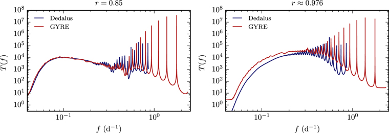
Figure 4. Comparison of the transfer function calculated in GYRE (red) and Dedalus (blue) for ℓ = 1 motions for a 10 M⊙ model near the ZAMS. In both panels, the Dedalus transfer functions are divided by 6. In the left (right) panel, we plot the transfer function where the luminosity is evaluated at r = 0.85R⋆ (r ≈ 0.976R⋆). With the normalization factor of one-sixth, there is excellent agreement at r = 0.85R⋆ between the two methods for low frequencies, and the two curves follow the same trends at higher frequencies. We believe the differences between the calculations at higher frequencies and also at r ≈ 0.976R⋆ is due to different in boundary conditions between the two calculations.
Download figure:
Standard image High-resolution imageThe transfer functions measured with the two numerical techniques are very similar. At low frequencies, the transfer functions are very small, and there are regularly spaced peaks at high frequencies.
However, the peaks are at different frequencies in the two codes. We believe this is due to differences in boundary conditions. At the surface, GYRE assumes no lagrangian pressure fluctuations, and a perturbed Stefan–Boltzmann equations; in Dedalus we set the radial velocity and eulerian entropy perturbation to zero at r ≈ 0.976R⋆. At the inner boundary, GYRE includes a convection zone, whereas the Dedalus domain does not. We do not expect the standing modes of the two problems to be the same, so the peaks in the transfer function should be at different frequencies. Note that there is always a Dedalus peak between every pair of GYRE peaks; this suggests that the period-spacing between the modes in the two calculations is very similar. Also recall that the amplitude of the four highest-frequency peaks in Dedalus are lower bounds on the transfer function, as we were not able to integrate long enough to establish the height of the peak. For this reason, we also did not calculate the transfer function in Dedalus for frequencies greater than ≈1 days−1.
The two calculations' transfer functions also have different amplitudes. In both panels of Figure 4, we divided the Dedalus transfer function by six. With this normalization, we find excellent agreement between the amplitudes of the two signals at r = 0.85R⋆. We expect the Dedalus transfer function to be larger because the waves in Dedalus are excited at r ≈ 0.216R⋆, whereas in GYRE we excited waves between r = 0.25R⋆ and r = 0.27R⋆. However, the waves only amplify by a factor of ≈2 between these points. Future work should examine the remaining difference in normalization between the calculations. In this work, we do not use the transfer function in any way that depends on its overall normalization.
We believe the difference between the normalization of the transfer functions calculated at r ≈ 0.976R⋆ is also due to differences in outer boundary conditions. It appears that the choice of boundary condition in Dedalus leads to luminosity fluctuations which are smaller by a factor of ≈3 at the upper boundary than the choice used in GYRE. We find that the eigenfunctions in both codes match very well until they reach the surface. This explains the agreement at r = 0.85R⋆.
Although there are some differences between the GYRE and Dedalus calculations, we find them to be minor. In fact, it may even be surprising that the agreement is so good, given the completely different numerical methods and the various inconsistent assumptions made in the two calculations. This good agreement gives us confidence in the main features of the transfer function: the transfer function is small at low frequencies due to damping, and is characterized by regularly spaced peaks due to standing modes at high frequencies.
Appendix G: Transfer Functions for Stars of Different Masses and Evolutionary Stages
In Figure 5, we plot the transfer function, calculated using GYRE, for a range of stellar models of different ages and initial masses. We only plot the transfer function for ℓ = 1 so it is easier to identify the trends with mass and age. The ℓ = 1 modes are expected to dominate the disk-averaged luminosity variation, as higher ℓ modes have significant cancellation. The three ages we include correspond to core hydrogen fractions of 0.66 (near the ZAMS), 0.33 (labeled "mid"), and nearly zero (TAMS). In all cases, we find a smooth transfer function corresponding to traveling waves at low frequencies. These waves are strongly damped, so the transfer function is small. At higher frequencies, the transfer function is dominated by regularly spaced peaks corresponding to standing modes.
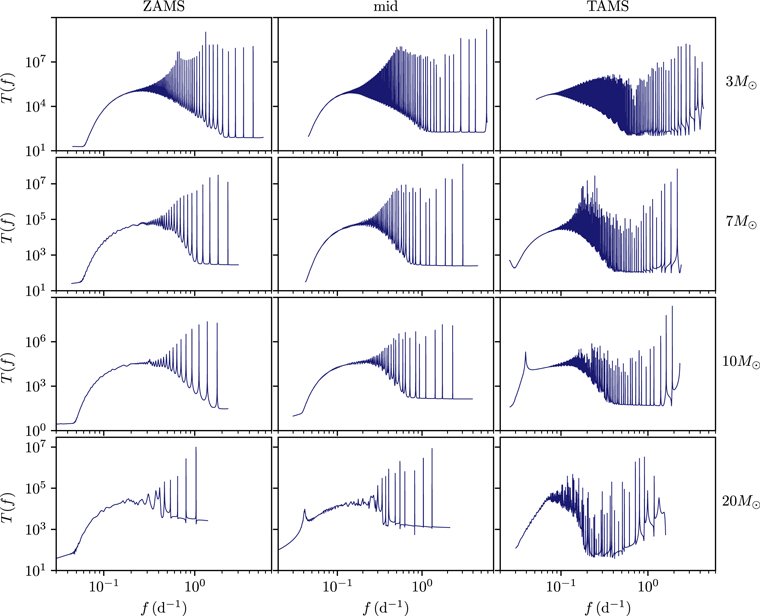
Figure 5. Transfer functions calculated in GYRE for ℓ = 1 modes, for stellar models of different masses and ages. The three ages correspond to core hydrogen fractions of 0.66 (near the ZAMS), 0.33 (labeled "mid"), and nearly zero (TAMS). Less-massive stars have less radiative damping, and thus have more standing modes than more massive stars. Radiative damping is also weaker at TAMS. However, all models show the same characteristic patterns: at low frequencies, the transfer function is smooth but small due to efficient wave damping, whereas at high frequencies, there are regularly spaced peaks corresponding to standing modes.
Download figure:
Standard image High-resolution imageMore massive stars have fewer standing-mode peaks. This is because the luminosity of these stars is larger, so radiative damping is more important. Thus, damped traveling waves exist at higher frequencies for higher-mass stars. Nevertheless, there are always several weakly damping standing modes, at least up to 20 M⊙. Lower-mass stars have an extremely large number of weakly damped standing modes. It is likely that ≈100 days TESS or K2 observations of 3 M⊙ stars would not be able to resolve most the individual standing-mode peaks. However, lower-mass stars also have a larger Brunt–Väisälä frequency, so g-modes extend to higher frequency. We thus believe that standing modes peaks with frequencies ∼4–5 days−1 should be detectable in observations of ≈3 M⊙ stars, if such waves were efficiently excited by convection.
There are only minor changes in the transfer function as the stars evolve from the ZAMS to midway between ZAMS and TAMS. The frequencies of the highest modes increase modestly, and radiative damping becomes somewhat weaker, leading to more standing modes. However, we find substantial changes when the stars reach TAMS. Radiative damping becomes significantly weaker at TAMS, leading to many more standing modes. The frequency spacing between the modes also seems smaller. Thus, it may be more difficult to detect individual standing modes for stars at the TAMS.
Several of our transfer functions have an abrupt change of slope at ≈0.05 day−1, e.g., ZAMS stars ≥7 M⊙. This is a numerical effect; this feature changes magnitude and frequency range when we change the resolution of the modes, the number of modes used, etc. The Dedalus calculation shows the transfer function decreases smoothly past these frequencies (see Figure 4, left panel). We believe the uptick in the transfer function for our 7 M⊙ TAMS model at the lowest frequencies is also due to this type of numerical error. For our 3 M⊙ TAMS model, we were not able to calculate the transfer function at low frequencies due to repeated floating-point exception errors thrown by GYRE.
At high frequencies, the transfer functions are dominated by very sharp peaks corresponding to standing modes. For many stellar models, the transfer function between these peaks seems to be nearly constant. We do not understand this behavior, but note that it seems to be robust to changes in numerical parameters, e.g., the resolution of the modes, the number of modes used, etc. It is unlikely that the behavior of the transfer function between the peaks have any observational implications.
Finally, we note that our 10 M⊙ TAMS model and 20 M⊙ "mid" model have well-defined peaks at ≈0.04 day−1. These appear to be numerically robust. We do not have a physical understanding of these features. If these features are physical, they may be detectable in long-duration observations of massive stars.
Appendix H: Overall Spectrum Normalization
Both LQ and R spectra have the normalization (Lecoanet & Quataert 2013; Rogers et al. 2013)

where Fw is the total wave flux, and Fc is the convective flux. The efficiency of wave generation is given by  , the convective Mach number, which we calculate using ωc/N0, where ωc is the convective frequency, and N0 is a typical value of the Brunt–Väisälä frequency in the radiative zone. The wave flux is dominated by waves near the convective frequency ωc and ΛH/rRCB ∼ 1, where rRCB and H are the radius and the scaleheight at the radiative–convective boundary, and
  as above. Thus, we have

where ur is the radial velocity of waves with frequencies near ωc and  , and ρRCB is the density at the radiative–convective boundary. We define
  , and
, and  . Then we have

Recall that this estimate is only for the most energetic waves with frequencies near ωc and  .
.
We can now combine this with the predicted frequency and wavenumber scalings (Section 2). The predictions for the radial velocity spectra are

To evaluate these expressions, we calculate the average convective velocity using
where Lc is the convective luminosity. The convective angular frequency is  , and the convective frequency is
  . We use
  as our estimate of the Brunt–Väisälä frequency.
We calculate each of these terms using our 10 M⊙ MESA model near the ZAMS. We find  ,
,  ,
,  , and fc ≈ 0.018 days−1. Thus, the theoretical predictions for the radial velocities are


For comparison, in Figure 2, we use a multiplying prefactor of 5 × 10⁻⁸ R⋆/d for the R spectrum, and 2 × 10⁻¹¹ R⋆/d for the LQ spectrum. Thus, the R spectrum predicts surface variability that is many orders of magnitude higher than what is observed. It may seem that the LQ spectrum predicts a similar magnitude to the observed variability, even if the shape of the spectrum is very different. However, we believe this is likely coincidental, as the very steep frequency dependence of the LQ spectrum makes it difficult to predict the overall amplitude of the spectrum. For instance, if we had used a different definition of the convective frequency, leading to a change by 2π, the overall amplitude of the spectrum could be as low as 2 × 10⁻¹⁴ or as high as 3 × 10⁻⁹. However, such a change in the definition of the convective frequency would lead to a very minor change in the R spectrum, because it has a very weak dependence on fc. This illustrates the need to calibrate the spectrum and convective frequency from 3D simulations of core convection.
Appendix I: Rotation
We have not included the effects of rotation in any of our calculations. Rotation plays an important role in the convective excitation of internal waves (Mathis et al. 2014). First, rotation can strongly constrain the convection, leading to flows that mostly align with the rotation axis (e.g., Augustson et al. 2016). This will modify the wave excitation process. Second, rotation changes the internal waves themselves. The eigenvalue problem for oscillation modes is 1D without rotation, but becomes 2D with rotation. This is because rotation couples together modes with different spherical harmonic degree ℓ, but does not couple modes with different azimuthal degree m. Oscillation modes with rotation can have non-trivial latitudinal structure.
Because of the 2D nature of the oscillation problem with rotation, it is difficult to calculate the transfer function. However, we will comment on some expected properties of the transfer function with rotation. Internal waves cannot propagate at the poles for f < 2/Trot, where Trot is the rotation period (not to be confused with the transfer function, T). The waves concentrate closer and closer to the equator in the limit that fTrot/2 goes to zero. These waves will cause negligible surface variability in stars observed from the poles. It is likely that at least some of the stars observed in B19 are observed nearly pole-on. These stars would show very little power at frequencies less than 2/Trot if the low-frequency variability was due to waves. However, a sharp decline in variability at low frequencies due to rotation is not observed in any of the stars, again suggesting that the variability is not due to waves.
If rotation is sufficiently weak (i.e., f ≫ 2/Trot), then oscillation modes are Doppler-shifted by rotation,  , where m is the azimuthal degree of the mode. If the convection is approximately isotropic, energy will be distributed between the different m modes evenly. Thus, each peak in the non-rotating transfer function will be evenly split into 2ℓ + 1 peaks under the influence of weak rotation. This will cause more peaks in the spectrum, and will change the spacing between peaks.
To illustrate these two effects, we plot rotationally modified surface luminosity spectra in Figure 6. This requires choosing nominal rotation periods for massive stars. Dufton et al. (2013) and Ramírez-Agudelo et al. (2013) measured the rotation velocities of B & O type stars as part of the VLT-FLAMES Tarantula Survey. In both cases, they find rotation velocities around 100–300 km s−1. Assuming a typical radius of 10R⊙, these roughly correspond to rotation rates of 2–5 days. This is in line with Nielsen et al. (2013), who reported a typical photometric rotation period for B stars of around 4 days. With this in mind, we consider two possible rotation periods, 2 days and 5 days, to demonstrate the possible effects of rotation. For frequencies less than 2/Trot (shaded in gray) we do not modify the spectrum. However, waves at these frequencies would be localized near the equator, and would have negligible surface manifestation for stars viewed pole-on. For frequencies greater than 2/Trot, we split the power of each peak evenly into 2ℓ + 1 peaks with frequencies f + m/Trot for  , assuming the weak-rotation limit. This leads to more peaks at high frequencies, and a more complicated spectrum. However, most of the individual peaks should still be resolved by the observations, so the theoretical spectra still do not resemble the smooth observed spectra of B19.

Figure 6. Luminosity variation spectrum for EPIC 234517653 from B19, and two rotationally modified theoretical spectra, for two different rotation periods, Trot. For frequencies f < 2/Trot, shaded in gray, waves can only propagate near the equator, and there will be negligible luminosity variations for stars observed pole-on. For higher frequencies, rotation produces Doppler-shifts, leading to more peaks. Although there are more peaks, their frequency spacing is large enough to be resolved by the observations.
Download figure:
Standard image High-resolution image
Footnotes
- 12
At the same time, the collective effect of gravity modes could also explain the macroturbulent velocities in these stars (Aerts et al. 2009).