In-situ Switchback Formation in the Expanding Solar Wind

The recent perihelion passes of Parker Solar Probe (PSP) have revealed a highly dynamic near-Sun solar wind (Bale et al. 2019; Kasper et al. 2019). A particularly extreme feature compared to solar-wind plasma at greater distances is the abundance of "switchbacks": sudden reversals of the radial magnetic field associated with sharp increases in the radial plasma flow (Neugebauer & Goldstein 2013; Horbury et al. 2018, 2020). Such structures generally maintain a nearly constant field strength $| {\boldsymbol{B}}|$, despite large changes to ${\boldsymbol{B}}$. It remains unclear how switchbacks originate and whether they are caused by sudden or impulsive events in the chromosphere or corona (e.g., Roberts et al. 2018; Tenerani et al. 2020).

In this Letter, our goal is to illustrate that turbulence with strong similarities to that observed by PSP develops from simple, random initial conditions within the magnetohydrodynamic (MHD) model. Using numerical simulations, we show that constant-$| {\boldsymbol{B}}|$ radial-field reversals arise naturally when Alfvénic fluctuations grow to amplitudes that are comparable to the mean field. We hypothesize that the effect is driven by magnetic-pressure forces, which, by forcing $| {\boldsymbol{B}}|$ to be nearly constant across the domain (Cohen & Kulsrud 1974; Vasquez & Hollweg 1998), cause large-$\delta {B}_{\perp }/{B}_{0}$ fluctuations to become discontinuous (Roberts 2012; Valentini et al. 2019). The effect is most pronounced around β ∼ 1 (where β is the ratio of thermal to magnetic pressure). Due to the radial expansion of the solar wind, initially small-amplitude waves propagating outward from the chromosphere naturally evolve into such conditions (van Ballegooijen et al. 2011; Perez & Chandran 2013; Montagud-Camps et al. 2018). We solve the MHD "expanding-box" equations (Grappin et al. 1993), which approximate a small patch of wind moving outward in the inner heliosphere. We deliberately keep the simulations simple, initializing with random superpositions of outward-propagating waves, assuming a constant wind velocity, and using an isothermal equation of state. That this generic setup reproduces many features of the turbulence and field statistics seen by PSP strongly suggests that switchbacks form in situ in the solar wind and are not remnants of impulsive or bursty events at the Sun.

We solve the isothermal MHD equations in the "expanding-box" frame (Grappin et al. 1993), which moves outward in the radial (x) direction at the mean solar-wind velocity, while expanding in the perpendicular (y and z) directions due to the spherical geometry. We impose a mean anti-radial (sunward) field ${{\boldsymbol{B}}}_{0}=-{B}_{x0}\hat{{\boldsymbol{x}}}$, with initial Alfvén speed ${v}_{{\rm{A}}}={B}_{x0}/\sqrt{4\pi \rho }$. The mass density ρ, flow velocity ${\boldsymbol{u}}$, and magnetic field ${\boldsymbol{B}}$ evolve according to

$$\begin{eqnarray}&&{\partial }_{t}\rho +\tilde{{\rm{\nabla }}}\cdot (\rho {\boldsymbol{u}})=-2\displaystyle \frac{\dot{a}}{a}\rho ,\end{eqnarray} \tag{ 1 }$$

$$\begin{eqnarray}\begin{array}{rcl}{\partial }_{t}{\boldsymbol{u}}+{\boldsymbol{u}}\cdot \tilde{{\rm{\nabla }}}{\boldsymbol{u}} & = & -\displaystyle \frac{1}{\rho }\tilde{{\rm{\nabla }}}\left[{c}_{s}^{2}(t)\rho +\displaystyle \frac{{B}^{2}}{8\pi }\right]\\ & & +\displaystyle \frac{{\boldsymbol{B}}\cdot \tilde{{\rm{\nabla }}}{\boldsymbol{B}}}{4\pi \rho }-\displaystyle \frac{\dot{a}}{a}{\mathbb{T}}\cdot {\boldsymbol{u}},\end{array}\end{eqnarray} \tag{ 2 }$$

$$\begin{eqnarray}&&{\partial }_{t}{\boldsymbol{B}}+{\boldsymbol{u}}\cdot \tilde{{\rm{\nabla }}}{\boldsymbol{B}}={\boldsymbol{B}}\cdot \tilde{{\rm{\nabla }}}{\boldsymbol{u}}-{\boldsymbol{B}}\tilde{{\rm{\nabla }}}\cdot {\boldsymbol{u}}-\displaystyle \frac{\dot{a}}{a}{\mathbb{L}}\cdot {\boldsymbol{B}}.\end{eqnarray} \tag{ 3 }$$

Here ${\mathbb{T}}=(0,1,1)$ and ${\mathbb{L}}=(2,1,1)$, $a(t)=1+\dot{a}t$ is the current perpendicular expansion with $\dot{a}/a$ the expansion rate, and $\tilde{{\rm{\nabla }}}\equiv ({\partial }_{x},{a}^{-1}{\partial }_{y},{a}^{-1}{\partial }_{z})$ is the gradient operator in the frame comoving with the expanding flow. The equation of state is isothermal, but with a sound speed c_s(t) that changes in time to mimic the cooling that occurs as the plasma expands (for adiabatic expansion, ${c}_{s}^{2}\,\propto \,a{(t)}^{-4/3}$). A detailed derivation of Equations (1)–(3) is given in, e.g., Grappin et al. (1993) and Dong et al. (2014). The anisotropic expansion causes plasma motions and magnetic fields to decay in time. Those that vary slowly compared to $\dot{a}/a$ scale as ${B}_{x}/\sqrt{\rho }\,\propto \,{a}^{-1}$, ${B}_{\perp }/\sqrt{\rho }\propto {a}^{0}$, u_x ∝ a⁰, ${u}_{\perp }\propto {a}^{-1}$, with ρ ∝ a⁻² (Grappin & Velli 1996). In contrast, for small-amplitude Alfvén waves with frequencies $\gg \dot{a}/a$, ${B}_{\perp }/{B}_{x}\propto {a}^{1/2}$, and ${u}_{\perp }/{v}_{{\rm{A}}}\propto {a}^{1/2}$. By appropriate parameter choices, we ensure that it is primarily this latter WKB effect that leads to large $\delta {B}_{\perp }/{B}_{0}$ waves in our simulations. The former non-WKB effect preferentially grows ${{\boldsymbol{B}}}_{\perp }/\sqrt{\rho }$ compared to ${{\boldsymbol{u}}}_{\perp }$, thus acting like a reflection term for largest-scale waves and aiding in the generation of turbulence.

2.1. General Considerations

2.2. Numerical Methods

2.3. Simulation Parameters and Initial Conditions

Our simulations are listed in Table 1. Each starts with randomly phased, "outward-propagating" (z⁺) Alfvén waves with ${{\boldsymbol{u}}}_{\perp }={{\boldsymbol{B}}}_{\perp }$ and u_x = 0. The initial normalized fluctuation amplitude $\langle {B}_{\perp 0}^{2}\rangle /{B}_{x0}^{2}=\langle {B}_{y0}^{2}+{B}_{z0}^{2}\rangle /{B}_{x0}^{2}$ in each simulation varies between 0.2 and 1. To explore the range of power spectra that might be present in the low corona (see, e.g., van Ballegooijen et al. 2011; Chandran & Perez 2019), we consider three types of initial magnetic power spectra ${E}_{\perp 0}$(k) in our simulations: (i) isotropic spectra peaked at large scales, including Gaussian spectra $[{E}_{\perp 0}(k)\propto \exp (-{k}^{2}/{k}_{0}^{2})$ with ${k}_{0}=12/{L}_{\perp }]$ and ${E}_{\perp 0}(k)\propto {k}^{-3};$ (ii) isotropic spectra with equal power across all scales $[{E}_{\perp 0}(k)\propto {k}^{-1}$]; and (iii) critically balanced spectra ${E}_{\perp 0}({k}_{\perp },{k}_{\parallel })\propto {k}_{\perp }^{-10/3}\exp (-{k}_{\parallel }{L}_{\perp }^{1/3}/{k}_{\perp }^{2/3})$, which we denote with the shorthand "${k}_{\perp }^{-5/3},{k}_{\parallel }^{-2}$" in Table 1, corresponding to the one-dimensional perpendicular and parallel spectra in the critical-balance model (Goldreich & Sridhar 1995; Cho et al. 2002). We avoid imposing any specific features on the flow or field (e.g., large-scale streams; Shi et al. 2020). Two additional simulation parameters are ${c}_{s}^{2}(t)$, which determines β through $\beta =8\pi {c}_{s}^{2}(t)\langle \rho /{B}^{2}\rangle$, and the expansion rate

$$\begin{eqnarray}&&{{\rm{\Gamma }}}_{\mathrm{sim}}\equiv \displaystyle \frac{\dot{a}}{a}\displaystyle \frac{{L}_{x}}{{v}_{{\rm{A}}}},\end{eqnarray} \tag{ 4 }$$

which is the ratio of outer-scale Alfvén time ${L}_{x}/{v}_{{\rm{A}}}$ to expansion time ${(\dot{a}/a)}^{-1}$. In our simulations, Γ_sim is constant because ${v}_{{\rm{A}}}$ ∝ a⁻¹, while $\dot{a}$ and L_x are constant.³

Table 1.  Properties of the Simulations Studied in This Work (β is Shown in Figure 1(a))

Name	Resolution	Code	$(\displaystyle \frac{{L}_{x}}{{L}_{\perp }^{i}},\tfrac{{L}_{\perp }^{f}}{{L}_{\perp }^{i}})$	$\displaystyle \frac{\dot{a}}{a}\tfrac{{L}_{x}}{{v}_{{\rm{A}}}}$	$\displaystyle \frac{\langle {B}_{\perp 0}^{2}\rangle }{{B}_{x0}^{2}}$	Spectrum
SW-GS	4803	Snoopy	(4, 10)	2	0.2	${k}_{\perp }^{-5/3}$, ${k}_{\parallel }^{-2}$
SW-Gaus	4803	Snoopy	(4, 10)	2	0.2	Gaussian
SW-s1	4803	Snoopy	(4, 10)	2	0.2	k−1
SW-GS-LR	2403	Snoopy	(4, 10)	2	0.2	${k}_{\perp }^{-5/3}$, ${k}_{\parallel }^{-2}$
β1-Gaus-HR	540 × 11202	Athena++	(1, 4)	0.5	1.0	Gaussian
β1-GS	280 × 5402	Athena++	(1, 4)	0.5	1.0	${k}_{\perp }^{-5/3}$, ${k}_{\parallel }^{-2}$
β1-Gaus	280 × 5402	Athena++	(1, 4)	0.5	1.0	Gaussian
β1-s1	280 × 5402	Athena++	(1, 4)	0.5	1.0	k−1
$\beta 1$-s3	280 × 5402	Athena++	(1, 4)	0.5	1.0	k−3
$\beta 0.1$-GS	280 × 5402	Athena++	(1, 4)	0.5	1.0	${k}_{\perp }^{-5/3}$, ${k}_{\parallel }^{-2}$
β0.02-GS	280 × 5402	Athena++	(1, 3)	0.5	1.0	${k}_{\perp }^{-5/3}$, ${k}_{\parallel }^{-2}$
β35-GS	280 × 5402	Athena++	(1, 4)	0.5	1.0	${k}_{\perp }^{-5/3}$, ${k}_{\parallel }^{-2}$
β1-$\dot{a}0.2$	280 × 5402	Athena++	(1, 4)	0.2	1.0	${k}_{\perp }^{-5/3}$, ${k}_{\parallel }^{-2}$
β1-$\dot{a}0$	280 × 5402	Athena++	(1, 1)	0	1.0	${k}_{\perp }^{-5/3}$, ${k}_{\parallel }^{-2}$

Note. ${L}_{\perp }^{i}$ and ${L}_{\perp }^{f}$ are the initial and final perpendicular box size.

Download table as:  ASCIITypeset image

Since most of the fluctuations propagate away from the Sun at speed ${v}_{{\rm{A}}}$ in the plasma frame, we map position x in the simulation to time t in the perihelion (zero-radial-velocity) PSP frame by setting

$$\begin{eqnarray}&&t=\displaystyle \frac{x}{U+{v}_{{\rm{A}}}}+{\rm{constant}}.\end{eqnarray} \tag{ 5 }$$

We then convert from simulation units to physical units by equating $\dot{a}/a$ in the simulations with U/r. We set r = 35R_⊙, U = 300 km s⁻¹, and ${v}_{{\rm{A}}}$ = 115 km s⁻¹, values that approximate the conditions during PSP's first perihelion pass (Bale et al. 2019; Kasper et al. 2019). The parallel box length L_x then corresponds via Equation (4) to the physical length scale 4.8 × 10⁶Γ_sim km. An outward-propagating Alfvén wave with parallel wavelength L_x has a frequency

$$\begin{eqnarray}&&\displaystyle \frac{U+{v}_{{\rm{A}}}}{{L}_{x}}=8.7\times {10}^{-5}{\left(\displaystyle \frac{{{\rm{\Gamma }}}_{\mathrm{sim}}}{0.5}\right)}^{-1}\mathrm{Hz}\end{eqnarray} \tag{ 6 }$$

in the spacecraft frame. The smallest resolvable parallel wavelength, approximately four times the grid scale, corresponds to an Alfvén-wave frequency $({N}_{\parallel }/4)\times (U+{v}_{{\rm{A}}})/{L}_{x}$, where N_∥ is the number of grid points in the x direction.

The Snoopy simulations, labeled SW-#, are designed to optimize property (i) of Section 2.1. They start from small-amplitude waves, $\langle {B}_{\perp 0}^{2}\rangle /{B}_{x0}^{2}=0.2$, and expand by a factor of a_f/a_i = 10 to reach large normalized amplitudes. We prescribe non-adiabatic temperature evolution ${c}_{s}^{2}(t)=0.35{t}^{-1}$ for these runs, causing β to increase from β ≈ 0.2 to β ≈ 1 (Figure 1(a)), in approximate agreement with near-Sun predictions from the model of Chandran et al. (2011) with parameters chosen to match conditions seen by PSP (see Chen et al. 2020). The amplitude increases broadly as expected, with some dissipation, as shown in Figure 1(b). In contrast, the Athena++ simulations (labeled β#-#) are designed to explore the basic physics of expanding-box turbulence at a range of β values. They are limited to a_f/a_i ≲ 4 by numerical instabilities, which necessitates starting from larger wave amplitudes, $\langle {B}_{\perp 0}^{2}\rangle /{B}_{x0}^{2}=1.0$. The fluctuations rapidly (within less than an Alfvén time) develop broadband turbulence and near-constant $| {\boldsymbol{B}}|$, resembling that at later times in the Snoopy runs. The temperature evolution in these runs is adiabatic (${c}_{s}^{2}(t)\propto {a}^{-4/3}$), so β remains nearly constant (Figure 1(a)). We choose Γ_sim = 0.5 for most simulations so that wave growth is mostly in the WKB regime, although it proved necessary to use an elongated box (${L}_{x}=4,\dot{a}=0.5;{{\rm{\Gamma }}}_{\mathrm{sim}}=2$) in the Snoopy simulations because of the enhanced dissipation over longer simulation times. We also explore a slower expansion rate Γ_sim = 0.2 (β1-$\dot{a}0.2$) and the same initial conditions with no expansion at all (β1-$\dot{a}0$).

Zoom In Zoom Out Reset image size

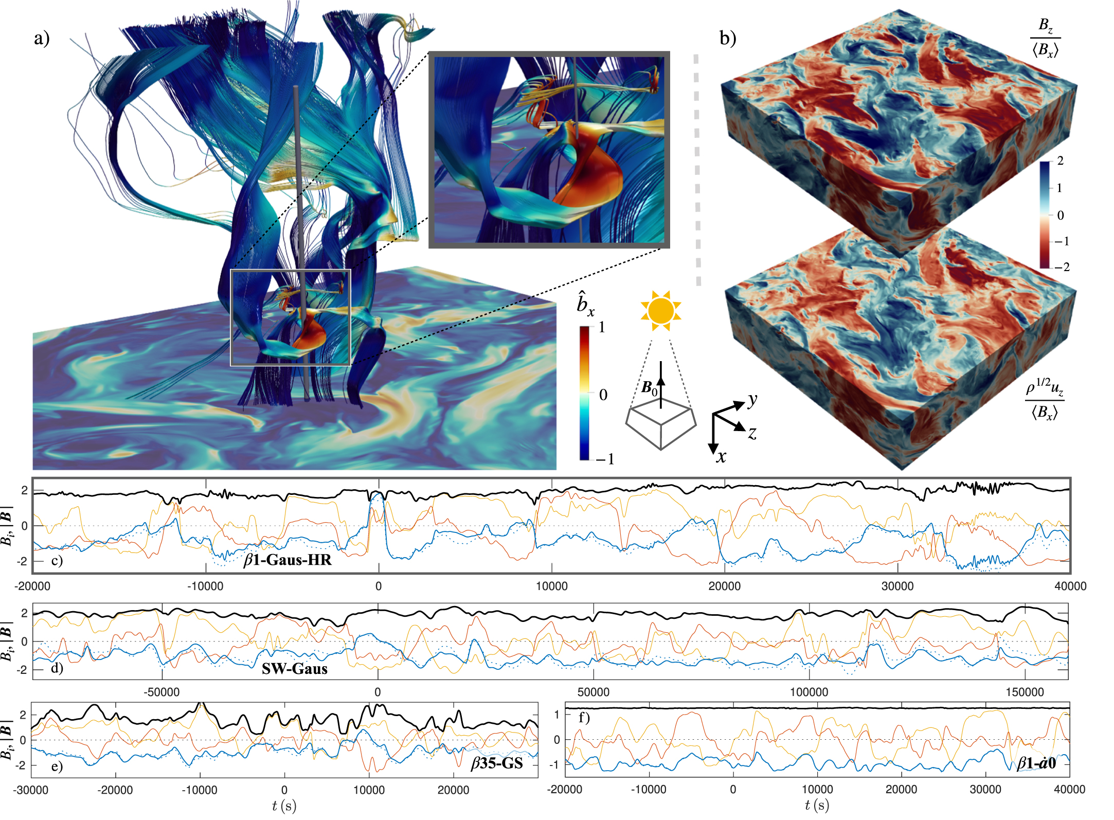
The evolved state from a selection of runs is shown in Figure 2, with a focus on β1-Gaus-HR. The field-line visualization shows a strong switchback with a complex, three-dimensional structure, as well as sharp, angular bends along other field lines. In the spacecraft-like trace shown below (panel (c)), we see that the switchback (around t = 0) results in a full reversal of the magnetic field to the antisunward direction ${\hat{b}}_{x}={B}_{x}/| {\boldsymbol{B}}| \approx +1$. The spacecraft remains in the B_x > 0 region for approximately 1000 s. The jumps at the boundaries of the switchback, with a scale of ∼100 s, are resolved by only 8–10 grid cells. Because of dissipation, this ∼100 s scale is likely around the simulation's minimum resolvable scale. Figure 2(c) also shows that $| {\boldsymbol{B}}|$ remains fairly constant despite large changes to ${\boldsymbol{B}}$, as ubiquitously observed in solar-wind data (Belcher & Davis 1971; Barnes 1981; Bruno & Carbone 2013).⁴ Time traces in the lower panels illustrate several other relevant simulations. SW-Gaus resembles β1-Gaus-HR, but with larger timescales and smoother variations due to the numerical method and lower resolution. In contrast, at high-β (β35-GS), the tendency to maintain constant $| {\boldsymbol{B}}|$ is almost eliminated, although there remains significant variation in B_x. With no expansion (β1-$\dot{a}0$) the lack of growth of $\delta {B}_{\perp }/{B}_{0}$ means there are only small fluctuations in B_x and no reversals, while $| {\boldsymbol{B}}|$ is nearly perfectly constant.

Zoom In Zoom Out Reset image size

More quantitative measures from all simulations are illustrated in Figure 3. We measure the "switchback fraction" with two methods. First, we simply count the fraction of cells with ${\hat{b}}_{x}\gt 0$, denoting this as ${f}_{{\hat{b}}_{x}\gt 0}$. Second, to quantify the prevalence of small-scale sharp changes in field direction, we calculate the probability density function of ${\hat{b}}_{x}$ increments, $| {\delta }_{{\ell }}{\hat{b}}_{x}| \equiv | {\hat{b}}_{x}({\boldsymbol{x}}+{\boldsymbol{\ell }})-{\hat{b}}_{x}({\boldsymbol{x}})|$ across scale ${\ell }=| {\boldsymbol{\ell }}| ={L}_{\perp }/68$ (∼8 grid cells), and define $P(| {\delta }_{{\ell }}{\hat{b}}_{x}| \gt 1)$ as the proportion of increments with $| {\delta }_{{\ell }}{\hat{b}}_{x}| \gt 1$. Two other useful statistics are the "magnetic compression,"

$$\begin{eqnarray}&&{C}_{{B}^{2}}\equiv \displaystyle \frac{\delta (| {\boldsymbol{B}}{| }^{2})}{{\left(\delta {\boldsymbol{B}}\right)}^{2}}=\displaystyle \frac{{\left\langle {\left(| {\boldsymbol{B}}{| }^{2}-\langle | {\boldsymbol{B}}{| }^{2}\rangle \right)}^{2}\right\rangle }^{1/2}}{\left\langle | {\boldsymbol{B}}-\langle {\boldsymbol{B}}\rangle {| }^{2}\right\rangle },\end{eqnarray} \tag{ 7 }$$

which measures the degree of spherical polarization ($| {\boldsymbol{B}}| \,={\rm{constant}}$),⁵ and the normalized fluctuation amplitude, which we define as $\langle {B}_{\perp }^{2}\rangle /\langle {B}_{x}{\rangle }^{2}=\langle {B}_{y}^{2}+{B}_{z}^{2}\rangle /\langle {B}_{x}{\rangle }^{2}$. We choose $\langle {B}_{x}\rangle$ to normalize the fluctuation amplitudes, as opposed to $\langle {B}_{x}^{2}\rangle$ or $\langle | {\boldsymbol{B}}| \rangle$, because $\langle {B}_{x}\rangle \propto {a}^{-2}$ is predetermined by the expansion and $\langle {B}_{\perp }^{2}\rangle /\langle {B}_{x}{\rangle }^{2}$ is not bounded from above (Matteini et al. 2018).

Zoom In Zoom Out Reset image size

Figure 3(a) plots ${C}_{{B}^{2}}$ and ${f}_{{\hat{b}}_{x}\gt 0}$ for all simulations and shows only modest changes to ${C}_{{B}^{2}}$ as the fluctuations evolve. Comparing our primary set of β ≈ 1 runs with β0.02, β0.1, and β35, we see—surprisingly—that ${C}_{{B}^{2}}$ is minimized around β ∼ 1. We also observe that ${C}_{{B}^{2}}$ increases with expansion rate (explaining the larger ${C}_{{B}^{2}}$ in Snoopy runs), probably due to non-WKB growth forcing ${B}_{\perp }\gt {u}_{\perp }$ at large Γ_sim, and that ${C}_{{B}^{2}}$ increases as the initial spectrum becomes steeper.

Figure 3(b) plots normalized fluctuation amplitude and $P(| {\delta }_{{\ell }}{\hat{b}}_{x}| \gt 1)$, illustrating that the increasing $\langle {B}_{\perp }^{2}\rangle$ caused by expansion causes the field to become more discontinuous. The good correlation with ${f}_{{\hat{b}}_{x}\gt 0}$ (inset) shows that similar processes lead to radial-field reversals. Comparing $P(| {\delta }_{{\ell }}{\hat{b}}_{x}| \gt 1)$ between cases β35-GS and β1-GS, which have identical initial wave spectra but very different ${C}_{{B}^{2}}$, tentatively supports the hypothesis that magnetic-pressure forces, in striving to keep $| {\boldsymbol{B}}|$ constant (Vasquez & Hollweg 1998; Roberts 2012), lead to a discontinuous field with switchbacks.⁶ We also see that: (i) at low β or with shallower initial spectra, the solutions are similarly discontinuous but the lower ${f}_{{\hat{b}}_{x}\gt 0}$ and $P(| {\delta }_{{\ell }}{\hat{b}}_{x}| \gt 1)$ is caused by these simulations not reaching such large amplitudes due to increased numerical dissipation (see also Figure 1(b)); (ii) lower-resolution simulations have a lower switchback fraction, especially in the Snoopy set (SW-Gaus-LR); and (iii) slower expansion (β1-$\dot{a}0.2$) causes larger ${f}_{{\hat{b}}_{x}\gt 0}$ and $P(| {\delta }_{{\ell }}{\hat{b}}_{x}| \gt 1)$ for similar amplitudes.

Magnetic-field and velocity spectra are shown in Figure 4. Figure 4(a), which pictures SW-Gaus, shows how the spectrum flattens to around $E({k}_{\perp })\sim {k}_{\perp }^{-1.5}$. This is expected and in line with previous results because non-WKB growth from expansion acts like a reflection term for large-scale waves, aiding in the development of turbulence (Grappin & Velli 1996). Figure 4(b) shows the evolution of the spectral slope from a number of simulations, illustrating the general trend toward slopes around $\sim {k}_{\perp }^{-1.5}$. Although there remain some differences depending on initial conditions, and a larger difference between kinetic and magnetic spectra than seen in the solar wind (Chen et al. 2020), the spectra in runs with nonzero $\dot{a}$ are quite similar to solar-wind spectra, despite the limited resolution of the simulations. In contrast, simulation β1-$\dot{a}0$ exhibits continual steepening of the spectrum due to grid dissipation and shows no tendency to develop solar-wind-like turbulence (this is also true with $\dot{a}=0$ and large-amplitude $\langle {B}_{\perp 0}^{2}\rangle /{B}_{x0}^{2}=4$ initial conditions, which have ${f}_{{\hat{b}}_{x}\gt 0}\ne 0;$ not shown). Finally, we note that the turbulence exhibits scale-dependent anisotropy similar to standard Alfvénic turbulence (Goldreich & Sridhar 1995; not shown).

Zoom In Zoom Out Reset image size

Figure 5 illustrates the shape of the most intense structures in β1-Gaus-HR (other cases are similar). We compute ${{\boldsymbol{n}}}_{\perp }\,=\hat{{\boldsymbol{x}}}\times \hat{{\boldsymbol{b}}}$ and ${{\boldsymbol{n}}}_{2}={\hat{{\boldsymbol{n}}}}_{\perp }\times \hat{{\boldsymbol{b}}}$, and use these to calculate the PDF of structures' length scales along field lines (${\left|\hat{{\boldsymbol{b}}}\cdot {\rm{\nabla }}\hat{{\boldsymbol{b}}}\right|}^{-1}$) and in the perpendicular directions (${\left|{\hat{{\boldsymbol{n}}}}_{\perp }\cdot {\rm{\nabla }}\hat{{\boldsymbol{b}}}\right|}^{-1}$ and $| {\hat{{\boldsymbol{n}}}}_{2}\cdot {\rm{\nabla }}\hat{{\boldsymbol{b}}}{| }^{-1}$). A rotational discontinuity is characterized by the scale of variation along $\hat{{\boldsymbol{b}}}$ being comparable to variation in the other directions, while a tangential discontinuity varies more rapidly in the directions perpendicular to $\hat{{\boldsymbol{b}}}$ (Neugebauer 1984). By filtering to include only regions of very large gradient as measured by the Frobenius norm ($| {\rm{\nabla }}\hat{{\boldsymbol{b}}}{| }^{-1}\leqslant | {\rm{\nabla }}{\hat{{\boldsymbol{b}}| }}_{\mathrm{cut}}^{-1}=4{L}_{\perp }/{N}_{\perp };$ solid lines), we see that many of the most intense structures do not exhibit sharp changes along $\hat{{\boldsymbol{b}}}$, as evidenced by the lack of a sharp peak in the PDF of $| \hat{{\boldsymbol{b}}}\cdot {\rm{\nabla }}\hat{{\boldsymbol{b}}}{| }^{-1}$ at $| {\rm{\nabla }}\hat{{\boldsymbol{b}}}{| }_{\mathrm{cut}}^{-1}$ (unlike the PDFs of $| \hat{{\boldsymbol{n}}}\cdot {\rm{\nabla }}\hat{{\boldsymbol{b}}}{| }^{-1}$). This shows that the most intense structures are generally tangential discontinuities, consistent with the simulated flyby and switchback illustrated in Figure 2(a).

Zoom In Zoom Out Reset image size

The key question that arises from our study is whether expansion and spherical polarization generically cause Alfvén waves propagating outward from the Sun to develop abrupt radial-magnetic-field reversals by the time they reach r = 35R_⊙, even if the initial wave field is smooth. The answer to this question is crucial for assessing what can be inferred about chromospheric and coronal processes from PSP measurements. Although we cannot rule out switchback formation in the low solar atmosphere, the simplicity of the in situ formation hypothesis is compelling, so long as it is consistent with observations. Our calculations clearly reproduce important basic features, including sudden Alfvénic radial-field reversals and jets, constant-$| {\boldsymbol{B}}|$ fields, and spectra around E(k) ∼ k^−1.5. On the other hand, our simulations do not quite reach ${f}_{{\hat{b}}_{x}\gt 0}$ ≈ 6%, as observed in PSP encounter 1 (Bale et al. 2019). This discrepancy, however, may simply result from lack of expansion or scale separation: ${f}_{{\hat{b}}_{x}\gt 0}$ depends on resolution (Figure 3), particularly for the Snoopy runs, which were designed to approximate the evolution of a solar-wind plasma parcel. Similarly, simulation β1-$\dot{a}0.2$, which probes smaller scales,⁷ exhibits larger ${f}_{{\hat{b}}_{x}\gt 0}$ and $P(| {\delta }_{{\ell }}{\hat{b}}_{x}| \gt 1)$ for similar $\delta {B}_{\perp }/{B}_{0}$. More detailed comparison to PSP fluctuation statistics will be left to future work (Chhiber et al. 2020; Dudok de Wit et al. 2020; Horbury et al. 2020).

The range of magnetic compressibility ${C}_{{B}^{2}}$ in our simulations broadly matches PSP observations on the relevant scales. A more intriguing prediction is the dependence of ${C}_{{B}^{2}}$ on β (Figure 3(a)), which may be a fundamental property of MHD turbulence. While the tendency for magnetic pressure to reduce δ$| {\boldsymbol{B}}|$ has been studied in a variety of previous works (e.g., Cohen & Kulsrud 1974; Barnes 1981; Vasquez & Hollweg 1996, 1998; Matteini et al. 2015), we believe that our observation that this tendency is strongest at β ∼ 1 is new. The increase in ${C}_{{B}^{2}}$ at high β is unsurprising: thermal pressure forces dominate and interfere with the magnetic-pressure driven motions that would act to reduce δ$| {\boldsymbol{B}}|$ (absent extra kinetic effects; Squire et al. 2019). At low β, however, the larger ${C}_{{B}^{2}}$ is more puzzling; we speculate on two possible reasons. First, the theory of Cohen & Kulsrud (1974) for Alfvénic discontinuities predicts a nonlinear time that approaches zero at β ∼ 1 because magnetic pressure resonantly drives parallel compressions that reduce δ$| {\boldsymbol{B}}|$. It is, however, unclear how this mechanism operates in a spectrum of oblique waves. Second, predicted parametric-decay growth rates increase at low β (Sagdeev & Galeev 1969; Goldstein 1978; Malara et al. 2000; Del Zanna 2001), which may disrupt the constant-$| {\boldsymbol{B}}|$ state and increase ${C}_{{B}^{2}}$ (although this remains unclear; see Cohen & Dewar 1974; Primavera et al. 2019). Parametric-decay processes may also aid in the development of turbulence (Shoda et al. 2019). This physics, along with the role of magnetic pressure in producing discontinuous fields and switchbacks, will be investigated in future work.

We show, using expanding-box compressible MHD simulations, that a spectrum of low-amplitude Alfvén waves propagating outward from the Sun naturally develops into turbulence with many similarities to that observed in the recent perihelion passes of Parker Solar Probe. Some features that are reproduced by our simulations include the presence of abrupt radial-magnetic-field reversals (switchbacks) associated with jumps in radial velocity, nearly constant magnetic-field strength, and energy spectra with slopes around ${k}_{\perp }^{-1.5}$. We present two sets of simulations with complementary numerical methods: the first (SW-# in Table 1) follows a parcel of plasma through a factor-of-10 expansion, with waves growing from linear to nonlinear amplitudes; the second (β#-#) explores the dependence of expansion-driven turbulence on initial conditions, β, and expansion rate.

Our key results can be summarized as follows:

• (i)  
  Switchbacks can form "in situ" in the expanding solar wind from low-amplitude outward-propagating Afvénic fluctuations that grow in normalized amplitude due to radial expansion. This indicates that PSP observations are broadly consistent with a natural state of large-amplitude imbalanced Alfvénic turbulence. The strongest switchbacks are tangential-like discontinuities.
• (ii)  
  The magnetic field develops correlations between its components in order to maintain constant $| {\boldsymbol{B}}|$ (Vasquez & Hollweg 1998). We show that this effect, which has been extensively documented in observations, is strongest at β ∼ 1, absent at high β, and reduced for β ≪ 1.
• (iii)  
  Imbalanced Alfvénic turbulence, with energy spectra $\sim {k}_{\perp }^{-1.5}$ and scale-dependent anisotropy, develops from homogeneous, random, outward-propagating Alfvén waves in the compressible expanding-box model.

We hypothesize that (i) results from (ii)—i.e., that switchbacks result from the combination of spherical polarization and expansion-induced growth in $\delta {B}_{\perp }/{B}_{0}$—because discontinuities are a natural result of large-$\delta {B}_{\perp }/{B}_{0}$ fluctuations with constant $| {\boldsymbol{B}}|$ (Roberts 2012; Valentini et al. 2019).

To more thoroughly assess the in-situ switchback-formation hypothesis and compare detailed statistical measures with observations, two important numerical goals for future work are to run to larger expansion factors without excessively fast expansion or high dissipation, and to reach the steady state where turbulent dissipation balances expansion-driven wave growth. This will require long simulation times at high resolution. Including mean-azimuthal-field growth (the Parker spiral) and/or improved expansion models (e.g., Tenerani & Velli 2017) may also be necessary. Theoretically, significant questions remain regarding the mechanisms for reducing δ$| {\boldsymbol{B}}|$(Cohen & Kulsrud 1974; Vasquez & Hollweg 1998).

We thank Stuart Bale, Chris Chen, Tim Horbury, Justin Kasper, Benoit Lavraud, Lorenzo Matteini, Anna Tenerani, and Marco Velli for helpful discussions. Support for J.S. and R.M. was provided by Rutherford Discovery Fellowship RDF-U001804 and Marsden Fund grant UOO1727, which are managed through the Royal Society Te Apārangi. B.C. was supported in part by NASA grants NNX17AI18G and 80NSSC19K0829 and NASA grant NNN06AA01C to the Parker Solar Probe FIELDS Experiment. High-performance computing resources were provided by the New Zealand eScience Infrastructure (NeSI) under project grant uoo02637 and the PICSciE-OIT TIGRESS High Performance Computing Center and Visualization Laboratory at Princeton University. This work was started at the Kavli Institute for Theoretical Physics in Santa Barbara, which is supported by the National Science Foundation under grant No. NSF PHY-1748958.