


Abstract
The amplitude of the 11 yr solar cycle is well known to be subject to long-term modulation, including sustained periods of very low activity known as Grand Minima. Stable long-period cycles found in proxies of solar activity have given new momentum to the debate about a possible influence of the tiny planetary tidal forcing. Here, we study the solar cycle by means of a simple zero-dimensional dynamo model, which includes a delay caused by meridional circulation as well as a quenching of the α-effect at toroidal magnetic fields exceeding an upper threshold. Fitting this model to the sunspot record, we find a set of parameters close to the bifurcation point at which two stable oscillatory modes emerge. One mode is a limit cycle resembling normal solar activity including a characteristic kink in the decaying limb of the cycle. The other mode is a weak sub-threshold cycle that could be interpreted as Grand Minimum activity. Adding noise to the model, we show that it exhibits Stochastic Resonance, which means that a weak external modulation can toss the dynamo back and forth between these two modes, whereby the periodicities of the modulation get strongly amplified.
Export citation and abstract BibTeX RIS

Original content from this work may be used under the terms of the Creative Commons Attribution 4.0 license. Any further distribution of this work must maintain attribution to the author(s) and the title of the work, journal citation and DOI.
1. Introduction
It is well known that the Sun's magnetic activity has a period of almost 11 yr (the Schwabe cycle) with polarity reversals around the maximum of each solar cycle. While the amplitudes of the different cycles may vary a lot, as measured by the (weighted) number of sunspots, the period around 11 yr is very stable. Superimposed on this basic 11 yr cycle are longer cycles, some of which have been known for a long time, such as the Gleissberg cycle (87 yr) and the Suess-deVries cycle (208 yr). The former modulates the amplitude of the Schwabe cycle, whereas the latter might be related to the recurrence of Grand Minima—time intervals extending over several cycles with few to no sunspots and much more reduced solar activity (e.g., McCracken et al. 2013).
The analysis of proxy data such as radio-nuclide time-series obtained from tree rings and ice cores has revealed the existence of many more long-period cycles in the history of magnetic solar activity (Berggren et al. 2009; Steinhilber et al. 2012). It is interesting to note that some of these cycles were already known from lake sedimentology and dendrochronology (e.g., Briffa et al. 1992; Kuma et al. 2019). Using high-precision C14 data, Brehm et al. (2021), Miyahara et al. (2021), and Usoskin et al. (2021) have recently presented detailed reconstructions of the history of the solar cycle.
In this Letter we study the variability of solar activity by means of a simple zero-dimensional dynamo model previously used by Wilmot-Smith et al. (2006). Despite its simplicity, this model incorporates two important features of the solar dynamo. One feature is the limitation of the operation of the α-effect to a window Bmin < B < Bmax, for the toroidal magnetic field strength, as suggested by Ferriz-Mas et al. (1994). Adding sufficient noise to the model, the lower threshold Bmin can lead to an on–off dynamo resembling realistic solar activity that is interspersed with Grand Minima (Schmitt et al. 1996). The second important feature that we consider is a time delay that accounts for the effect of meridional circulation, a key ingredient in any Babcock–Leighton (BL) type model (Babcock 1961; Leighton 1969).
The resulting system of delay ordinary differential equations (ODEs) shows interesting dynamic phenomena, which completely disappear if the time delay is set to zero. We show that it exhibits two fundamentally different modes of stable oscillation, which can co-exist for certain ranges of parameter values. One mode, which we call the weak mode, is characterized by frequencies and amplitudes that are subject to periodic or chaotic modulation, depending on the parameter values. The fact that chaos can occur in a system of only two coupled ODEs is indeed due to the delay, which effectively renders the system infinite-dimensional. For certain parameter ranges, the weak mode remains mostly below Bmax (hence the name). As Bmax defines the critical field strength that toroidal flux tubes need to exceed in order to be able to rise toward the solar surface and form sunspots, we posit that the weak mode could explain the mechanism behind Grand Minima, which is in line with the observation that solar magnetic activity (i.e., the operation of the solar dynamo) does not stop during these periods (Beer et al. 1998). The other mode is a stable limit cycle and shows no modulation. As the amplitude of this mode can be much larger than Bmax; we call it the strong mode. This mode exhibits a characteristic kink in its decaying limb, which is also present in observational sunspot data, and which stems from the toroidal field exceeding Bmax. This effect has been pointed out before by Stix (1972).
Within the range of parameters where both stable modes co-exist, the dynamo can switch easily between them upon adding sufficient noise to the equations. That is, the dynamo shows intermittent behavior similar to the one described in Schmitt et al. (1996), except that it is Bmax rather than Bmin that is responsible for this behavior, and the Grand Minima would correspond to a stable sub-threshold oscillatory mode rather than the zero mode of the dynamo equations.
Near the bifurcation point where the new oscillatory mode appears, the basins of attraction of the two modes are particularly susceptible to external perturbations. This phenomenon is known as Stochastic Resonance (Benzi et al. 1981; McNamara & Wiesenfeld 1989). In recent years some controversy has arisen around the suggestion that the tidal effect exerted by the planets might have an influence on the solar magnetic activity (e.g., Abreu et al. 2012; Stefani et al. 2019, 2020, 2021). Indeed, it is remarkable that many of the long-period cycles that we find in proxies of solar activity can also be found in time-series of the torque exerted by the planets on the Sun (Abreu et al. 2012). This has motivated us to study, by means of a simple dynamo model, whether a tiny (external) modulation can imprint its periodicities onto the mode-switching of the dynamo, whereby they are greatly amplified by Stochastic Resonance. However, the specific question whether Stochastic Resonance is actually powerful enough to amplify the tiny tidal forcing enough to effectively have an effect on the operation of the dynamo is not addressed in this Letter and requires further investigation.
2. Stochastic Resonance in BL-type Dynamos
Following Wilmot-Smith et al. (2006) we model the solar dynamo with two coupled delay ODEs, for the toroidal and poloidal fields, respectively:


where Ω0 is a characteristic value of the angular velocity distribution Ω(r, θ) in the convection zone, L is a characteristic length of variation, α0 is a characteristic value of the α-effect, and τ is the diffusion timescale. The two delays T0 and T1 represent the timescales set by meridional circulation and the rising time of buoyant flux tubes, respectively. The nonlinear function f(B) essentially restricts the α-effect that keeps the dynamo alive to a range Bmin ≲ B(t) ≲ Bmax. Following Wilmot-Smith et al. (2006), we use the symmetric box-shaped function (Figure 1)

and we have fixed the limiting values somewhat arbitrarily to Bmin = 1 and Bmax = 10.
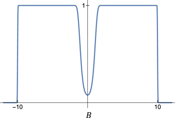
Figure 1. Function f(B) limiting the alpha effect, with Bmin = 1 and Bmax = 10.
Download figure:
Standard image High-resolution imageEquations (1) and (2) can be combined to a second-order delay ODE, for the dominant toroidal field

where q = (T0+T1)/τ and we have set the time unit such that τ = 1. The dimensionless dynamo number  (see e.g., Charbonneau 2020) is the ratio of the source terms to the dissipative terms in the dynamo equations and is expressed as

There has been some discussion as to whether the dynamo is dominated by flux-transport (q < 1, e.g., Wilmot-Smith et al. 2006) or by diffusion (q > 1, e.g., Karak & Choudhuri 2011). Here we fix q = 0.82, which has been found in an attempt to fit model (4) to the sunspot record (see Figure 2). However, the phenomena that we describe here do not depend much on the particular value of q, and there are other values that lead to similar fits.

Figure 2. Fit of the sunspot record. The relative delay parameter was found to be q ≈ 0.82, and the dynamo number  was found to be close to the upper critical point (compare with Figure 3).
Download figure:
Standard image High-resolution imageAbove Bmax, the rhs of (4) is almost zero, hence the dynamo turns into a critically damped oscillator when B(t) exceeds Bmax. For now, let us ignore the lower limit Bmin and consider f(B) to be a single box stretching from −Bmax to Bmax. While B(t) remains below Bmax, the system is then almost linear. We start with a linear stability analysis of the trivial solution B(t) = 0 of Equation (4). Therefore, we turn Equation (4) into a first-order equation for  . The linearized equation (f = 1) reads
  , with
With the ansatz
x
(t) = eλ
t
x
0 we find the characteristic equation,  , to be

Writing λ = μ + iν, the stability of the zero solution is determined by the sign of μ. For the bifurcation point μ = 0, we derive from (6) the condition for the cycle-frequency ν to be given by equation

The solution with the lowest value, ν*, defines the critical dynamo number, at which the zero solution becomes unstable to be given by

At this point, Equation (4) has the harmonic solution B(t) = Asinν*t. However, the amplitude A is unstable. It decays to zero, for dynamo numbers below  , and would grow unbounded for higher values, if it were not for Bmax, which stabilizes the solution again. Simulations show that, at
  , the zero solution bifurcates to the harmonic solution B(t) ∝ sinν*t, with amplitude close to Bmax. Further increasing
  leads to periodic and chaotic modulations of both the amplitude and the period. (Figure 3). This period-doubling route to chaos is a robust feature of BL-type dynamos, which has been observed also in simpler iterative map models as well as more complicated spatially resolved models (Charbonneau et al. 2005). The amplitude-modulations are superimposed to an increasing trend, starting at around Bmax. The period, on the other hand, is modulated around the linear solution ν*. For the sake of simplicity, we refer to this entire mode of oscillation as the weak mode.

Figure 3. Field amplitudes B2 as a function of the dynamo number  , for q = 0.82, exhibiting the transition between the weak and the strong mode around
  . The inset shows the corresponding periods against
  (same units). Gray vertical lines indicate the dynamo number used for the realization in Figure 4.
Download figure:
Standard image High-resolution imageIf we introduce Bmin, this generic picture persists. However, the zero solution remains stable for dynamo numbers beyond  . Hence, there is a range of dynamo numbers, roughly between
  and
and  , for which the dynamo admits at least two stable modes (the weak mode and the zero mode).
For even larger values of the dynamo number, a fundamentally different mode of oscillation emerges (the branch in Figure 3 above dynamo number  ). This is a mode where B(t) is above Bmax most of the time and both the amplitude and the period are constant. We call it the strong mode. It is the stable limit cycle that appears when we approximate
  in Equation (4). This approximation is valid for large
  , where the cycle period is much larger than q. For smaller values of
  , the approximation fails and the system can no longer be approximated by a second-order ODE, hence the emergence of the chaotically modulated weak mode.
The cycles of the strong mode have a characteristic shape, similar to the large solar cycles that were observed in the sunspot records (Figure 2): a steep rising limb, followed by a falling limb with a kink. This shape has been interpreted as an effect of the B-field exceeding Bmax before by Stix (1972), albeit with a non-BL-type dynamo model. The fit in Figure 2 has been achieved through optimizing parameters q and  . Interestingly, the optimized value
  turned out to be quite close to the critical point where the strong mode becomes stable.
The strong and the weak mode can co-exist, over certain parameter ranges. For the q = 0.82 solution depicted in Figure 3, we could numerically verify the co-existence of the strong and the weak mode for dynamo numbers up to  . Adding sufficiently strong (additive) noise to the dynamo equations allows the system to randomly switch between these different stable modes of operation. Near the critical points, the basins of attraction of the modes are particularly susceptible to perturbations. Hence, near these points, a weak external modulation can alter the probabilities of mode-switching substantially and thus lead to a strong amplification of the cycles that are present in the modulation. We demonstrate this Stochastic Resonance numerically, operating our dynamo within the co-existence range of the strong and the weak mode. Therefore, we add a small periodic modulation, as well as additive white noise, to the dynamo Equation (4):
where  = 0.02 and η(t) is a white noise with co-variance
  . We choose the driving frequency ωd
such that it comprises about 15 dynamo cycles.
. We choose the driving frequency ωd
such that it comprises about 15 dynamo cycles.
Figure 4 shows a typical realization. The dynamo number  lies within the co-existence range of the strong and the weak mode. The relatively small noise amplitude of σ = 0.17 allows for occasional sustained periods of weak dynamo operation, not unlike the pattern observed in long records of solar activity derived from radio-nuclides (Steinhilber et al. 2012). Increasing the noise increases the frequencies of such Grand Minima-like episodes (not shown). Figure 5 compares the power spectrum of this realization against a realization without noise, but otherwise identical parameter values. The noise-induced amplification of the driver-mode, which is characteristic for Stochastic Resonance, is clearly visible. For this realization, the amplification appears to be mainly due to an amplitude modulation of the strong mode (inset in Figure 5). However, for stronger noise, it is dominated by the recurrence of weak-mode episodes, i.e., the recurrence of "Grand Minima" (not shown).
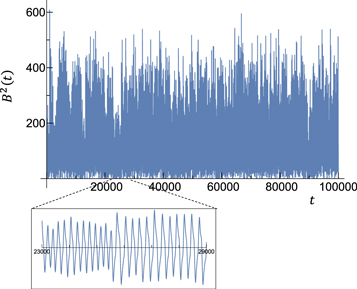
Figure 4. Realization from Equation (9), for q = 0.82,  and σ = 0.17. Magnetic energy B2(t) is plotted against time, the units of which are chosen such that the base period 2π/ν* ≈ 100 (resulting in τ ≈ 43). Several Grand Minima-like events are visible. The inset shows the typical shapes of the cycles, for a time interval exhibiting a mode-switch.
Download figure:
Standard image High-resolution image
Figure 5. Power spectral density (PSD) of the realization of Figure 4 (orange), compared to the spectrum of a realization without noise but otherwise using the same parameter values (blue). Stochastic Resonance leads to an amplification of the external driver represented by the peak at 1500. The inset shows the amplification on a small time interval.
Download figure:
Standard image High-resolution image
3. Discussion and Conclusions
We have demonstrated that a zero-dimensional dynamo model with delay and an upper threshold for the α-effect exhibits two fundamentally different stable oscillatory modes, which can co-exist for suitable parameter values. A similar observation has recently also been made by Tripathi et al. (2021). We believe that this is a generic feature that generalizes to more refined dynamo models of that type, which we plan to study in the future.
An upper threshold for the α-effect (usually called "α-quenching" in the literature and imposed ad hoc) naturally arises from the fact that, when the magnetic field strength of toroidal flux tubes lying beneath the bottom of the convection zone increases above a threshold value, the tubes become unstable, enter the convection zone from below, and buoyantly rise toward the surface (e.g., Schüssler et al. 1994). A delay is caused by the fact that the source layers for the α- and the Omega-effect are located at different places within the star.
Depending on the parameter values, the weak mode could produce few to no sunspots as is the case during Grand Minima, whereas the strong mode, with its characteristic kink, resembles active dynamo operation. We have also shown qualitatively that, upon adding noise to the model, a weak external driver can be greatly amplified through Stochastic Resonance, either via a switching between the two different modes or via amplitude modulation of the strong mode. Thus, Stochastic Resonance could provide a generic explanation for the appearance of long-period cycles in the record of solar activity: they owe their existence to the amplification of a weak external forcing.
The effect of stochastic fluctuations in the operation of the solar dynamo has been considered by a number of authors (see e.g., Hoyng 1988). In particular, Hoyng (1993) and Moss et al. (2008) considered the effect of multiplicative noise terms in mean-field dynamo models, and demonstrated that they can lead to large amplitude fluctuations including Grand Minima-like episodes. Our approach is distinctly different in that it suggests a delay-induced bi-stability of the dynamo operation as a possible explanation for the Grand Minima, which in addition allows for Stochastic Resonance.
Here we have only investigated the effect of a modulation of the dynamo number  , but any other way of modulating the basins of attraction of the two different modes should have a similar effect. Where to insert the modulation depends on the kind of external driver and on the physical effect it has on the dynamo, which is not the subject of this Letter (but see, e.g., Stefani et al. 2019, 2020, 2021).
Future research will have to focus on a quantitative comparison between the observed and simulated features of solar magnetic activity. The features that are of interest to Stochastic Resonance include the dominant long-period cycles in solar activity, but also the location and duration of each Grand Minima episode (and possibly also Grand Maxima). Other relevant features include the shape of solar cycles. Here we have only considered the characteristic kink in their decaying limb, but there are others, such as the Waldmeier relations relating rise- an decay-times of cycles to their amplitudes (Waldmeier 1939), which need to be included in a full-fledged quantitative comparison.
Approximate Bayesian Computation, which is based on comparing relevant observed features with their counterparts from stochastic simulations, lends itself to this task. A parameter sample from the Bayesian posterior could even open the perspective of predicting the amplitudes of future solar cycles including an estimate of the uncertainty.
C.A. and S.U. acknowledge support by the Swiss Data Science Center under the BISTOM project. A.F.M. acknowledges support by the Spanish Science Ministry under project RTI2018-096886-B-C51. The authors are grateful to Benjamín Montesinos, Jürg Beer, and Wolfgang Schmidt for useful comments. They would also like to thank an anonymous referee for interesting suggestions.