


 t 19, 4000 Liège, Belgium

Abstract
On 2020 April 29, the near-Earth object (52768) 1998 OR2 experienced a close approach to Earth at a distance of 16.4 lunar distances (LD). 1998 OR2 is a potentially hazardous asteroid of absolute magnitude H = 16.04 that can currently come as close to Earth as 3.4 LD. We report here observations of this object in polarimetry, photometry, and radar. Our observations show that the physical characteristics of 1998 OR2 are similar to those of both M- and S-type asteroids. Arecibo's radar observations provide a high radar albedo of  0.29 ± 0.08, suggesting that metals are present in 1998 OR2 near-surface. We find a circular polarization ratio of μc = 0.291 ± 0.012, and the delay-Doppler images show that the surface of 1998 OR2 is a top-shape asteroid with large-scale structures such as large craters and concavities. The polarimetric observations display a consistent variation of the polarimetric response as a function of the rotational phase, suggesting that the surface of 1998 OR2 is heterogeneous. Color observations suggest an X-complex taxonomy in the Bus–DeMeo classification. Combining optical polarization, radar, and two epochs from the NEOWISE satellite observations, we derived an equivalent diameter of D = 1.80 ± 0.1 km and a visual albedo pv = 0.21 ± 0.02. Photometric and radar data provide a sidereal rotation period of P = 4.10872 ± 0.00001 hr, a pole orientation of (332
 3 ± 5°, 207 ± 5°), and a shape model with dimensions of
  km.
km.
Export citation and abstract BibTeX RIS

Original content from this work may be used under the terms of the Creative Commons Attribution 4.0 licence. Any further distribution of this work must maintain attribution to the author(s) and the title of the work, journal citation and DOI.
1. Introduction
1998 OR2 (hereafter OR2) is an H = 16.04 (according to the Minor Planet Center (MPC); other determinations of the H magnitude include H = 15.6 ± 1, Masiero et al. 2021; H = 16.15 ± 0.1, Vereš et al. 2015; and H = 16.1 ± 0.2, Betzler & Novaes 2009) absolute magnitude near-Earth object (NEO) that was discovered in 1998 by the Near-Earth Asteroid Tracking (NEAT) NASA program (Pravdo et al. 1999). With a minimal orbital intersection distance (MOID) of 0.008 7 au and an estimated diameter around 1.8 km, OR2 is considered as a potentially hazardous asteroid (PHA; see Table 1 for the OR2 orbital elements). From the 174 currently known NEOs with H magnitude smaller than 16.1 (hence larger than OR2), OR2 has the fifth-smallest MOID. With MOID of 0.0030, 0.0042, 0.0044, and 0.0066 au, only (2201) Oljato, (85713) 1998 SS49, (1981) Midas, and (4179) Toutatis, respectively, have smaller MOID and are of the same size as or larger than OR2 (at an epoch of 2023 February 25 as the MOID of an asteroid is evolving with time). With a Δv = 6.5 km s −1, OR2 is also a good target for a space mission.
Table 1. Osculating Orbital Elements of OR2 at Epoch 60000 MJD (2023 February 25) Obtained with the JPL Horizons Service
| a | e | MOID | i | ω | Ω |
|---|---|---|---|---|---|
| (au) | (au) | (deg) | (deg) | (deg) | |
| 2.3804 | 0.5754 | 0.0087 | 5.8782 | 26.9415 | 180.1589 |
Note. https://ssd.jpl.nasa.gov/horizons/app.html.
Download table as: ASCIITypeset image
On 2020 April 29, OR2 experienced a close flyby to Earth at a distance of 16.4 lunar distances (LD) (0.0420 au) and reached a V magnitude of 10.8. This is the closest and brightest apparition since its discovery and until 2079 April 16, when it will get as close as 4.6 LD (0.01185 au).
Prior to the 2020 flyby, not much was known about the physical characteristics of OR2. Light-curves were obtained during its 2009 flyby at a distance of 70 LD (0.179 au). These light-curves showed low amplitude and were mostly dominated by noise due to the rather distant flyby. As a matter of fact, several publications reported inconsistent rotation period values. Betzler & Novaes (2009) reported a rotation period P = 3.198 ± 0.006 hr with an amplitude A = 0.29 ± 0.01 mag, while Koehn et al. (2014) and Skiff et al. (2019) (the Skiff et al. 2019 paper is actually a reanalysis of the same data as the Koehn et al. 2014 paper) found periods of P = 4.112 ± 0.002 hr and P = 4.1120 ± 0.000 6 hr with an amplitude of A = 0.16 ± 0.02 mag and 0.16 ± 0.01 mag, respectively. From the 2020 flyby, many light-curves have already been published that all confirm the 4.11 hr period (4.106 ± 0.003 hr for Warner & Stephens 2020b; 4.111 ± 0.001 hr for Franco et al. 2020; 4.112 ± 0.01 hr, 4.111 4 ± 0.0002 hr, and 4.113 3 ± 0.0009 hr for Warner & Stephens 2020a; 4.108 ± 0.001 hr for Aznar-Macías 2020; and 4.126 ± 0.179 hr for Battle et al. 2022). Colazo et al. (2021) are the only ones who found a significantly different period of 4.01 ± 0.02 hr.
OR2 has been classified as an Xk type in the Bus and Binzel taxonomy (Bus & Binzel 2002) using spectrophotometric observations (Somers et al. 2010). This classification was later confirmed during this flyby with visible spectroscopic data from the NEOROCKS project (Javier Licandro, private communication) and our own spectrophotometric observations obtained for this work (in this work, using colors observations, we obtain an X-complex classification). On the other hand, using a combination of visible (0.4–0.9 μ m; VIS) and near-infrared spectroscopy (0.9–2.5 μm; NIR), Battle et al. (2022) reported an Xn taxonomy. The difference between the previous classification is that the Xk and Xn types mainly differ in the NIR part of the spectrum, where the Xn types are flat and the Xk types are red-sloped. However, Battle et al. (2022) propose that the composition of OR2 is similar to S-type asteroids and explain its flatter spectrum (compared to regular S-type asteroids) by the evidence of shock darkening or impact melts on its surface.
In this paper, we are presenting a multitechnique observation campaign of OR2 that is showing that its physical properties are showing similarities to both M-type and S-type asteroids. We will see that OR2 is showing the characteristic of a metallic surface but is also displaying the presence of silicates as with other M-type asteroids (Fornasier et al. 2010; Landsman et al. 2018).
2. Observations
In this section we present our new observations of OR2 using three different techniques: optical polarimetry, photometry, and radar. These observations were conducted between 2020 January 5 and 2022 November 23.
2.1. Optical Polarimetry
We obtained optical polarimetric observations of OR2 with the Torino Polarimeter (ToPol) in 2020 February and April. ToPol is mounted on the Cassegrain focus of the 1.04 m Omicron telescope (C2PU facility) of the Calern Observatory located near the city of Nice in the South of France (MPC 010). ToPol is a wedged double Wollaston polarimeter that allows full characterization of the Stokes parameters I, Q, and U in one single observation. See Pernechele et al. (2012) and Devogèle et al. (2017) for more information about ToPol and Bendjoya et al. (2022) for a recent update on all the observations performed with ToPol.
In the case of atmosphereless bodies, the linear degree of polarization is defined as the difference between the intensity of the light having its polarization oriented perpendicular to the scattering plane (i.e., the plane containing the Sun–object–observer) and the intensity of the light having its polarization oriented in the scattering plane. This difference is then divided by the sum of the same parameters for normalization purposes. This parameter, often referred to as Pr , is then negative if the polarization is found to lie in the scattering plane or positive if it is perpendicular to it. See Belskaya et al. (2015) for a review and more information about asteroid polarimetry.
The linear degree of polarization of asteroids is directly dependent on the solar phase angle α (i.e., the Sun–object–observer angle). At low solar phase angle (typically <20°) the orientation of the polarization is found to be aligned with the scattering plane (Pr < 0). This part of the solar phase polarization curve is referred to as the negative polarization branch. For higher solar phase angles, the orientation of the polarization is found to be aligned with the plane perpendicular to the scattering plane (Pr > 0) with a transition (the inversion angle α0) usually occurring around α ∼ 20°.
During our observations, from 2020 February to April, the solar phase angle of OR2 varied from 30° to 78°, allowing for a detailed characterization of the positive polarization branch of the solar phase polarization curve. Figure 1 shows night averages of the observed polarization of OR2. The orange lines represent the best fit of an exponential-linear model to the data, with the width of the curve representing the uncertainties on the model fit (see Section 3.1 for the detailed discussion on how the fit was obtained and on its interpretation). A summary of the night average polarimetric observations is presented in Table 2.

Figure 1. Solar phase polarization curve of 1998 OR2 observed at the C2PU facility (Calern Observatory). Observations were carried out between 30° and 78° of solar phase angle. The linear part of the positive polarization branch is observed. The orange lines represent the best fits of an exponential-linear model, with the width of the curve representing the modeled uncertainties obtained using an MCMC routine.
Download figure:
Standard image High-resolution imageTable 2. Night Average Summary of 1998 OR2 Polarization Measurements (Pr )
| Date | V | Δ | r | α | Pr |
|---|---|---|---|---|---|
| (mag) | (au) | (au) | (deg) | (%) | |
| 2020 Feb 18 | 15.0 | 0.306 | 1.240 | 30.4 | 1.32 ± 0.12 |
| 2020 Feb 19 | 15.0 | 0.302 | 1.233 | 31.4 | 1.46 ± 0.22 |
| 2020 Feb 24 | 14.9 | 0.281 | 1.200 | 36.6 | 2.20 ± 0.14 |
| 2020 Apr 6 | 14.1 | 0.117 | 1.024 | 75.3 | 7.82 ± 0.10 |
| 2020 Apr 8 | 13.9 | 0.108 | 1.022 | 76.2 | 8.14 ± 0.10 |
| 2020 Apr 10 | 13.5 | 0.099 | 1.019 | 77.0 | 8.10 ± 0.08 |
| 2020 Apr 11 | 13.4 | 0.095 | 1.019 | 77.2 | 8.18 ± 0.08 |
| 2020 Apr 14 | 13.1 | 0.083 | 1.017 | 77.5 | 8.26 ± 0.10 |
| 2020 Apr 15 | 13.0 | 0.078 | 1.017 | 77.3 | 8.01 ± 0.08 |
| 2020 Apr 16 | 12.8 | 0.074 | 1.017 | 77.0 | 8.03 ± 0.08 |
| 2020 Apr 17 | 12.7 | 0.070 | 1.018 | 76.5 | 7.99 ± 0.08 |
| 2020 Apr 23 | 11.7 | 0.050 | 1.023 | 68.2 | 6.68 ± 0.08 |
| 2020 Apr 24 | 11.5 | 0.047 | 1.024 | 65.9 | 6.18 ± 0.08 |
| 2020 Apr 28 | 10.9 | 0.042 | 1.031 | 53.2 | 4.29 ± 0.08 |
Note. Δ and r correspond to the distances of the OR2 to Earth and the Sun, respectively. α is the solar phase angle. All parameters are listed for the mid-time of all observation nights.
Download table as: ASCIITypeset image
During the April observations, OR2 was continuously observed over several hours at a time to measure its linear degree of polarization as a function of time. During this period, OR2 was observable from the Calern Observatory for approximately 4–5 hr per night, allowing us to observe one full rotation every night. Figure 2 shows all polarimetric data of OR2 obtained between April 6 and April 24 phased according to its rotation period. The rotation-phase-locked variation can be seen with a relative amplitude of 5%–6% (peak-to-peak). See Section 3.2 for a discussion of Figure 2 and how it was obtained.
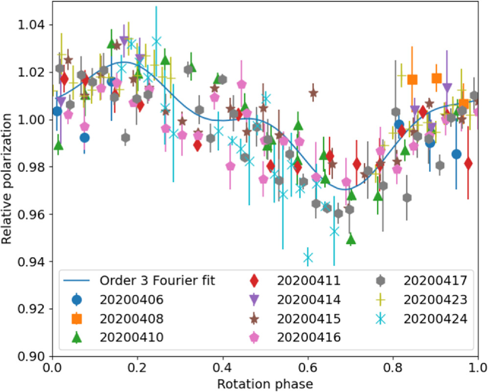
Figure 2. Plot of the relative polarization (linear degree of polarization divided by the best-fit model) as a function of the rotation phase of 1998 OR2 (with the different colors corresponding to different nights). A clear correlation can be seen with respect to the rotation phase, implying that the surface of 1998 OR2 is heterogeneous. The blue solid line represents the best Fourier fit of order 3.
Download figure:
Standard image High-resolution image2.2. Photometry
We observed OR2 in photometry during the close 2020 flyby but also during its oppositions far away from Earth in 2021 and 2022. During those apparitions, it was observable at lower solar phase angles than during the 2020 flyby, and they allowed us to fine-tune the shape model with observations at different viewing geometries. During the 2021 apparition, it only reached a magnitude of V = 21.0, but it was observable at a minimum solar phase angle of α = 07. During the 2022 apparition, it reached a magnitude of V = 20.6 with a minimum solar phase angle of α = 09.
Our photometric campaign involved 22 different telescopes located at different observatories over a wide range of Earth longitudes. The different telescopes are summarized in Table 3.
Table 3. Summary of All Facilities Used in This Work
| Facility | Diameter | Location | Filters |
|---|---|---|---|
| (m) | (MPC or lon/lat in deg) | ||
| Lowell Discovery Telescope | 4.3 | G37 | VR |
| TRAPPIST-North | 0.60 | Z53 | R |
| OWL-Net_MNG Observatory | 0.50 | O72 | B, V, R, I |
| OWL-Net_MAR Observatory | 0.50 | Z01 | B, V, R, I |
| OWL-Net_ISR Observatory | 0.50 | M33 | B, V, R, I |
| OWL-Net_USA Observatory | 0.50 | V15 | B, V, R, I |
| OWL-Net_KOR Observatory | 0.50 | P72 | B, V, R, I |
| Skalnaté Pleso Observatory | 0.61 | 056 | B, V, R |
| Teide Observatory (TAR2) | 0.46 | 954 | None |
| McDonald Observatory (LCO;fa07) | 1.0 | V39 | w |
| Teide Observatory (LCO;kb98) | 0.4 | Z21 | w |
| Haleakala Observatory (LCO;kb27) | 0.4 | T04 | r' |
| Siding Spring Observatory (LCO;kb28) | 0.4 | Q59 |

|
| Sutherland Observatory (LCO;fa16) | 1.0 | K91 |

|
| Isaac Aznar Observatory | 0.35 | Z95 | V |
| Roncevaux Observatory (RON) | 0.25 | 2.46/+48.28 | None |
| Linhaceira Observatory | 0.12 | 938 | UV and VIS cut filter |
| S. Maria de Montmagastrell | 0.41 | B74 | None |
| Harfleur Observatory (HAR) | 0.20 | 0.01/+49.60 | None |
| Les Barres Observatory | 0.35 | K22 | R |
| Deep Sky Chile Observatory (DSC) | 0.30 | 286.15/−30.53 | V |
| Chillou Observatory (CHI) | 0.20,0.25 | 0.20/+47.13 | None |
Note. The location is represented by the MPC code of the telescope or the longitude and latitude if no MPC code is available.
Download table as: ASCIITypeset image
At the 4.3 m Lowell Discovery Telescope (LDT; MPC G37), we used the Large Monolithic Imager in a 3 × 3 binning mode providing a plate scale of 0 36 pixel−1 and a square field of view of
  . The LDT was used during the 2021 and 2022 apparitions only to observe OR2 at low solar phase angles and to obtain light-curves at different viewing geometries. The 2021 and 2022 observations are the only observations with subobserver latitudes in the southern hemisphere of OR2. All LDT observations were obtained using a "VR" filter covering both the V and R photometric bands (bandpass from 0.480 ± 0.005 μm to 0.721 ± 0.005 μm) and have all been calibrated in the Sloan r band.
At the robotic TRAPPIST-North observatory (TN; MPC Z53), we used a 0.6 m robotic Ritchey–Chrétien design telescope operating at f/8 on a German equatorial mount (Jehin et al. 2011). The camera is an Andor IKONL BEX2 DD (060 pixel−1,  field of view). Images were obtained with a binning of 2 × 2 and a broadband Cousins R filter.
We used five telescopes from the Las Cumbres Observatory consortium of telescopes. We used two 1.0 m telescopes from the McDonald Observatory in Texas, USA (MPC code V39), and from the Sutherland Observatory in South Africa (MPC code K91). These two observatories have a similar telescope setup called Sinistro that captures a  field of view, sampled at a pixel scale of 0778 pixel−1 in the 2 × 2 binning mode. We also used three 0.4 m telescopes: one from the Siding Spring Observatory (MPC code Q59), one from the Teide Observatory (MPC code Z21), and one from the Haleakala Observatory (MPC code T04). All these telescopes are also identical and capture a
  field of view sampled at a pixel scale of 0571 pixel−1 in the 1 × 1 binning mode. All LCO observations were scheduled using the NEOExchange Target and Observation Manager (TOM; Lister et al. 2021), and images were reduced by the LCO pipeline (McCully et al. 2018) using standard bias, dark, and flat-field corrections. A combination of filters were used at these telescopes, the SDSS
  , and z' filters and the Pan-STARRS w filter (Hodapp et al. 2004).
The Optical Wide-field patroL Network (OWL-Net) is a network of five Richey–Chretien robotic telescopes of 0.5 m (Park et al. 2014). They are respectively located at the Songino in Mongolia (OWL-Net_MNG; MPC code O72), the Oukaimeden Observatory in Morocco (OWL-Net_MAR; MPC code Z01), the Wise Observatory in Israel (OWL-Net_ISR; MPC code M33), the Mount Lemmon Observatory in Arizona, USA (OWL-Net_USA; MPC code V15), and the Bohyunsan Observatory in Korea (OWL-Net_KOR; MPC code P72). OWL-Net observations were obtained with the BVRI Johnson–Cousins standard filters.
At the Teide Observatory in Tenerife (MPC code 954), we used TAR2, an f/2.8 0.46 m robotic telescope equipped with an SCMOS FLI Kepler KAF400 providing a resolution of 17 pixel−1. Due to the small aperture of the telescope, these observations were performed unfiltered.
Photometric observations of 1998 OR2 were also performed using the 0.61 m f/4.3 reflecting telescope at the Skalnaté Pleso Observatory in Slovakia (MPC code 056) and an SBIG ST-10XME CCD camera located at the primary focus. Photometric observations were done in the standard broadband Johnson–Cousins BVR filters. The observations were obtained using a 2 × 2 binning corresponding to a resolution of 1069 pixel−1.
We also made use of optical observations of OR2 from a group of amateur astronomers. All of these light-curves were collected by Raoul Behrend from the Observatoire de Genève and published on his website. 28 The OR2 data set contains observations from seven observers from Chile, France, Portugal, and Spain.
All data from LDT, TRAPPIST-N, OWL-Net, and Teide telescopes were reduced using the PHOTOMETRYPIPELINE (Mommert 2017) and were photometrically calibrated in their own filter in the case of the B, V, R, and I filters and in the Sloan r' band for the LDT VR filter and unfiltered observations from the Teide.
2.3. Radar Observations
Radar observations of OR2 in S band (2380 MHz; 12.6 cm) were obtained with the 305 m radio telescope at the Arecibo Observatory for 9 days between 2020 April 13 and 23. Radar observations consist of sending a circularly polarized signal to the asteroid and observing the signal that is reflected by the asteroid surface back to the observer. Upon reflection, the circularly polarized signal interacts with the surface, and the reflected signal can be found either with a circular polarization rotating in the opposite direction from the transmitted signal (OC) or in the same orientation (SC). Upon interaction on a smooth surface, the reflected signal is expected to be fully oriented in the opposite circular polarization, while multiple scattering on a rough terrain can result in the signal being polarized in the same orientation as the transmitted one or be depolarized owing to multiple scattering in random directions. As a consequence, the observed received signal can be found polarized in both the SC and OC channels. The measurement of the SC/OC ratio or circular polarization ratio (μc ) has been shown to provide information about the taxonomy (Benner et al. 2008), the surface roughness at scales comparable to the wavelength (Ostro et al. 1985), and the shape and size distribution of the particles (Virkki & Muinonen 2016; Virkki & Bhiravarasu 2019). See Hickson et al. (2021) for a recent study of radar polarimetry.
The radar observations were performed using several observing modes. The first mode is the continuous-wave (CW) mode. CW observations consist of sending a continuous unmodulated 2380 MHz circularly polarized signal to the asteroid, and the reflected signal is observed in both circular polarizations. Due to the motion and rotation of the target, the received signal is shifted in frequency compared to the transmitted signal, as a result of the Doppler effect. CW observations allow us to obtain information on the rotation state, speed of the object relative to Earth, radar albedo, and circular polarization ratio. They can also sometimes give clues about the presence of satellites. All the CW observations are summarized in Table 4, along with information that can be directly extracted from the spectra, such as the bandwidth (BW; maximum extent of the CW spectrum), the OC and SC cross sections (σSC, σOC), the radar albedos for the OC and SC spectra ( ,
,  ), and the circular polarization ratio (μc
). For the radar albedos (which is the observed radar cross section divided by the asteroid's projected area), we take into account the cross section from the shape model derived in this paper. For details about CW spectrum bandwidth, cross sections, and radar albedo definitions in the case of radar observations and how they are calculated for Arecibo Observatory observations, see Virkki et al. (2022).
), and the circular polarization ratio (μc
). For the radar albedos (which is the observed radar cross section divided by the asteroid's projected area), we take into account the cross section from the shape model derived in this paper. For details about CW spectrum bandwidth, cross sections, and radar albedo definitions in the case of radar observations and how they are calculated for Arecibo Observatory observations, see Virkki et al. (2022).
Table 4. Summary of OR2 CW Observations
| Date | Δ | Ecl. Lon | Ecl. Lat | BW | σOC |

| S/NOC | σSC |

| S/NSC | μc |
|---|---|---|---|---|---|---|---|---|---|---|---|
| (au) | (deg) | (deg) | (Hz) | (km2) | (km2) | ||||||
| 2020 Apr 13 22:36:22 | 0.087 | 122.2 | 9.2 | 9.2 | 0.845 ± 0.209 | 0.297 ± 0.079 | 175 | 0.243 ± 0.057 | 0.085 ± 0.022 | 6 | 0.287 ± 0.007 |
| 2020 Apr 16 22:49:31 | 0.074 | 126.3 | 5.7 | 8.5 | 0.697 ± 0.181 | 0.248 ± 0.069 | 137 | 0.216 ± 0.053 | 0.077 ± 0.020 | 9 | 0.310 ± 0.006 |
| 2020 Apr 17 22:20:39 | 0.071 | 127.9 | 4.3 | 7.5 | 0.819 ± 0.176 | 0.295 ± 0.070 | 189 | 0.240 ± 0.051 | 0.086 ± 0.020 | 14 | 0.293 ± 0.004 |
| 2020 Apr 18 22:18:38 | 0.067 | 129.8 | 2.6 | 7.5 | 0.931 ± 0.225 | 0.314 ± 0.082 | 196 | 0.247 ± 0.060 | 0.084 ± 0.022 | 17 | 0.265 ± 0.003 |
| 2020 Apr 19 22:27:35 | 0.063 | 132.0 | 0.8 | 6.8 | 0.874 ± 0.197 | 0.292 ± 0.072 | 192 | 0.260 ± 0.055 | 0.087 ± 0.020 | 20 | 0.297 ± 0.002 |
| 2020 Apr 20 23:37:30 | 0.059 | 134.4 | −1.4 | 6.3 | 0.844 ± 0.222 | 0.279 ± 0.078 | 121 | 0.247 ± 0.060 | 0.082 ± 0.021 | 16 | 0.292 ± 0.004 |
| 2020 Apr 21 23:37:22 | 0.056 | 137.2 | −3.7 | 5.3 | 0.835 ± 0.215 | 0.274 ± 0.094 | 82 | 0.249 ± 0.063 | 0.082 ± 0.022 | 11 | 0.298 ± 0.005 |
| 2020 Apr 22 23:22:16 | 0.053 | 140.2 | −6.3 | 4.6 | 0.982 ± 0.254 | 0.325 ± 0.090 | 70 | 0.272 ± 0.068 | 0.091 ± 0.024 | 9 | 0.281 ± 0.006 |
| 2020 Apr 23 22:53:50 | 0.050 | 143.7 | −9.1 | 3.5 | 0.940 ± 0.249 | 0.311 ± 0.107 | 56 | 0.281 ± 0.075 | 0.093 ± 0.031 | 9 | 0.299 ± 0.007 |
Note. Column (1): the mid-time of the observations. Column (2): the distance to Earth (Δ) in au of OR2 at mid-time. Columns (3) and (4): the ecliptic longitude and latitude in degrees. Column (5): the bandwidth (BW) of the CW spectrum in Hz. Columns (6) and (9): the cross section (σ) and its associated uncertainties in km2 for the OC and SC signal, respectively. Columns (7) and (10): the radar albedos ( ) for the OC and SC spectra, respectively (here we are taking into account the asteroid's geometric cross section from the shape model). Columns (8) and (11): the S/Ns of the OC and SC spectra, respectively. Column (12): the circular polarization ratios (μc
).
) for the OC and SC spectra, respectively (here we are taking into account the asteroid's geometric cross section from the shape model). Columns (8) and (11): the S/Ns of the OC and SC spectra, respectively. Column (12): the circular polarization ratios (μc
).
Download table as: ASCIITypeset image
It is interesting to note that the observed bandwidth of OR2 is decreasing by a factor of three over the 10 days of observations. We will see in Section 3.6 that this variation of the bandwidth allows us to obtain a reliable estimate of the spin axis orientation of OR2.
The second mode of radar observations is the delay-Doppler imaging mode. This mode consists of sending a modulated signal to the object and measuring the reflected signal. The modulation, often called binary phase-shift keying, consists of pseudo-random shifts of the phase by 180° at a fixed interval of time. The period of time between the potential shifts is called the baud length and defines the range resolution. The pseudo-random modulation is repeated after a period of time called the code length. The code length should be large enough that there are no ambiguities between two identical sequences received at the same time but reflected by part of the body at different distances (range) from the observer. Typically the code length (duration of the code times the speed of light) should be larger than the size of the object. As with the CW signal, the received signal is shifted in frequency owing to the Doppler effect, but in the case of the delay-Doppler imaging mode, the modulation of the signal also makes it possible to precisely time the round-trip time for the received signal. The delay-Doppler imaging mode thus allows us to construct a 2D image where the axes are the range (distance from the observer) and the Doppler shift. Based on the distance and expected signal from the target, several submodes of the delay-Doppler mode can be used. These submodes differ by their baud and code lengths. In this work, we used baud lengths of 4.0, 0.5, 0.2, 0.1, and 0.05 μs (see Table 5), corresponding to spatial resolutions of 600, 75, 30, 15, and 7.5 m, respectively. However, the produced images can have lower pixel height (spatial resolution of each pixel) if the data are sampled several times during a single baud. This is refered to as the number of samples per baud. Most of our images are sampled several times so that the image resolution is 7.5 m per pixel. For more details about radar observations, the reader can refer to Ostro (1993) and Virkki et al. (2022).
Table 5. Summary of OR2 Delay-Doppler Radar Observations
| Date | JD | Baud | SPB | IR | No. Scans | Δ | Ecl. Lon | Ecl. Lat |
|---|---|---|---|---|---|---|---|---|
| (μs) | (m) | (au) | (deg) | (deg) | ||||
| 2020 Apr 13 | 2458953.48723 | 4 | 2 | 600 | 21 | 0.087 | 122.21 | 9.20 |
| 2020 Apr 16 | 2458956.46366 | 4 | 2 | 600 | 6 | 0.074 | 126.31 | 5.67 |
| 2020 Apr 16 | 2458956.48569 | 0.5 | 1 | 75 | 15 | 0.074 | 126.34 | 5.64 |
| 2020 Apr 17 | 2458956.51994 | 0.2 | 4 | 7.5 | 13 | 0.074 | 126.40 | 5.59 |
| 2020 Apr 17 | 2458957.48687 | 0.1 | 2 | 7.5 | 48 | 0.070 | 128.40 | 4.10 |
| 2020 Apr 18 | 2458958.48593 | 0.1 | 2 | 7.5 | 52 | 0.067 | 129.93 | 2.53 |
| 2020 Apr 19 | 2458959.49569 | 0.1 | 2 | 7.5 | 51 | 0.063 | 132.08 | 0.66 |
| 2020 Apr 21 | 2458960.51042 | 0.1 | 2 | 7.5 | 6 | 0.059 | 134.52 | −1.45 |
| 2020 Apr 22 | 2458961.51644 | 0.05 | 1 | 7.5 | 34 | 0.056 | 137.26 | −3.80 |
| 2020 Apr 23 | 2458962.51415 | 0.05 | 1 | 7.5 | 37 | 0.053 | 140.35 | −6.40 |
| 2020 Apr 23 | 2458963.49082 | 0.05 | 1 | 7.5 | 51 | 0.050 | 143.79 | −9.22 |
Note. Columns (1) and (2): the calendar and Julian date, respectively, of when the observation was obtained. Column (3): the baud length in μs. Column (4): the number of samples per baud (SPB). Column (5): the image resolution (IR). Column (6): the total number of scans obtained during the observations. Column (7): the geocentric distance (Δ) of OR2 during the observations. Columns (8) and (9): the ecliptic longitude and latitude, respectively, of OR2 during the observations.
Download table as: ASCIITypeset image
The delay-Doppler images suggest that OR2 possesses a spheroidal shape or top shape (spheroidal with an equatorial ridge). Top-shaped asteroids are common in the NEO population, and several of them have been modeled using radar observations. One example is (101955) Bennu (Nolan et al. 2013), whose shape has been confirmed by the OSIRIS-REx mission in situ observations (Barnouin et al. 2019). A second example is (66391) Moshup (formerly known as 1994 KW4), which has been independently confirmed to be a top-shape asteroid by adaptive optics observations (Reddy et al. 2022). Finally, the recent DART impact showed that the asteroid (65803) Didymos is also top-shaped, as predicted by the radar-derived shape model (Naidu et al. 2020).
The radar delay-Doppler images of OR2 also display large-scale structures that suggest that it is diplaying large concavities. The main one is displayed in Figure 3 for three different epochs. Other structures suggesting deviations from pure top-shape models are shown in Figure 4 as small nonconvex features (concavities) on the leading edge of the delay-Doppler images. As for Figure 3, Figure 4 is displaying these structures for three different epochs and thus slightly different viewing geometries. The crater is also visible in Figure 4 on the left side of the images.
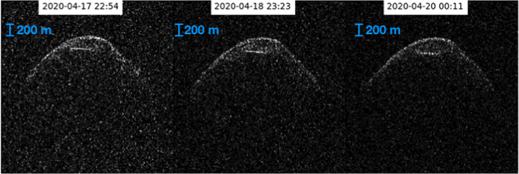
Figure 3. Delay-Doppler images of a large crater or concavity observed near the subradar point. These three images have been obtained on three different observing runs, showing that the structure repeats with the asteroid's rotation. Each image has been obtained with a 0.1 μs baud length at two samples per baud, resulting in each column pixel corresponding to 7.5 m on OR2.
Download figure:
Standard image High-resolution image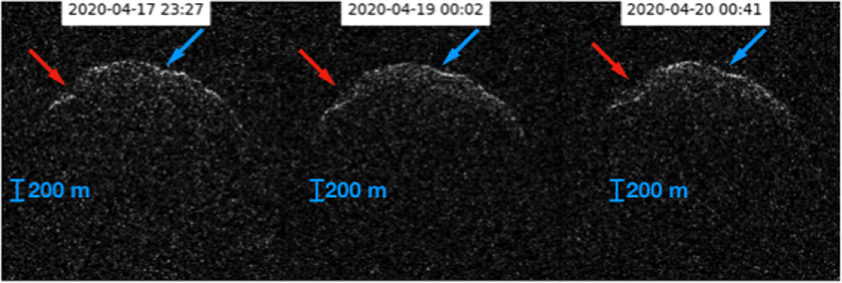
Figure 4. Delay-Doppler images of another structure (indicated by the blue arrow) that can be seen as a concavity close to the subobserver latitude. The structure can be seen at three different epochs, confirming that it repeats with the asteroid's rotation. On the left side of the images (indicated by the red arrow), the crater shown in Figure 3 can been seen. Each image has been obtained with a 0.1 μs baud length at two samples per baud, resulting in each column pixel corresponding to 7.5 m on OR2.
Download figure:
Standard image High-resolution image3. Results
In this section we will present the results obtained from the new observations of OR2.
3.1. Solar Phase Polarization Curve
The observations obtained in optical polarimetry allow us to construct a solar phase polarization curve spanning a large range of solar phase angles from 30° to 80°, allowing us to characterize the positive polarization branch. However, as all our measurements are displaying positive values of the P r parameter, we are not able to characterize the negative polarization branch.
To model the solar phase polarization curve, we used the exponential-linear model presented in Muinonen et al. (2009) and formulated as follows:

This model assumes that the positive polarization branch is characterized by a linear increase of the polarization while lower phases are modeled using an exponential behavior to model the negative polarization branch and the inversion angle that usually happens around 20° of solar phase angle. It also assumes that the polarization is null at zero solar phase angle. This mathematical model has been shown to satisfactorily represent the solar phase polarization curves of asteroids. However, the downside is that the parameters used to represent the solar phase polarization curves of asteroids (i.e., the inversion angle α0, the slope at the inversion angle, the maximum extent of the negative polarization branch ( ), and the phase at which it is occurring (
 )) are not parameters of the model. However, it is possible to derive these parameters based on the model parameters A, B, and C. Details on how these parameters are mathematically derived from the A, B, and C parameters are discussed in Muinonen et al. (2009), Cellino et al. (2015), and Devogèle et al. (2018b).
We are using a Markov Chain Monte Carlo (MCMC) fitting routine using the EMCEE Python package
29
to model the solar phase polarization curve using the exponential-linear model. As we do not possess observations below 30° of solar phase angle, we are using prior information based on the solar phase polarization curves of other asteroids. For this we are using the data set presented in Cellino et al. (2016). They analyzed the solar phase polarization curves of 60 asteroids. We are thus using the distribution of α0,  , and
, and  from Cellino et al. (2016) to constrain our fit to physical values for these parameters. As these three parameters are not independent of each other and can only take a small range of values for real asteroids, this prior information is highly important to obtain a realistic fit of the solar phase polarization curve when no data are available at low solar phase angles.
The fit to the data is presented in Figure 1 as the orange line, with the shaded area around the best-fit model representing the variance around the best model and thus the uncertainties. Even if we do not have data below 30° of solar phase angle, the use of the prior information allows us to still obtain valuable information on the inversion angle. The results of the MCMC fitting provide  ,
,  , and
, and  . Using the relations described in Devogèle et al. (2018b), we are obtaining an inversion angle of
  and a slope at the inversion angle of
  . According to the Cellino et al. (2015) relation linking the slope at the inversion angle determined with the exponential-linear model to the albedo, we find an albedo for OR2 of
  . This determination of the albedo should be taken with caution, as we do not have any measurements at solar phase angle lower than the inversion angle. However, this estimation is consistent with independent albedo determination using other techniques in this work (see Section 4.1).
3.2. Optical Polarization Time Series
The linear degree of polarization of the light scattered by an asteroid surface does not depend on its shape. As a result, polarization is almost never analyzed as a time series (like optical light-curves), but as a function of the solar phase angle as discussed in the previous section. However, in the case of OR2 we find that the polarization displays variations that are correlated with the rotation phase. In the following, to avoid confusion between the phase angle (i.e., the Sun–asteroid observer angle) and the phase of rotation (fraction of a rotation of the asteroid around itself), we will refer to the phase angle as the solar phase and the phase of rotation as the rotation phase. Due to the independence of the polarization from the shape, these variations should be triggered by heterogeneities of surface properties such as the albedo, composition, or grain size over the surface of OR2.
However, while we find that OR2 is displaying variations that are correlated with the rotation phase, as a first order, the polarization is still mainly dependent on the solar phase angle. If we expect variations that are due to heterogeneities on the surface (albedo or grain size variations), their amplitude are expected to be correlated with the absolute value of the polarization. As the solar phase angle is varying quickly from night to night and even during a single night, we need to correct for this variation. This correction is performed by first modeling the solar phase polarization curve using the exponential-linear model as explained in Section 3.1. We then normalize each individual observation to the polarization value provided by the best-fitted model.
To first assess whether the observed variations are correlated with the rotation phase of OR2, we ran a Lomb–Scargle periodogram using the relative polarimetric data. The result of the Lomb–Scargle periodogram shows the strongest peak for a period of P = 4.1145 hr consistent with the rotation period of OR2. Figure 5 shows the Lomb–Scargle periodogram using polarimetric data only.

Figure 5. Lomb–Scargle periodogram using the relative polarization data. The strongest peak of the periodogram corresponds to a period of P = 4.1145 hr consistent with the rotation period of OR2.
Download figure:
Standard image High-resolution imageAn independent check can also be performed using a Fourier series analysis. For this we are using a Fourier series of order 3 and try all the periods between 3.5 and 4.5 hr. We then compute the residuals between the fit of the Fourier seriesand the data and compute the χ2 taking into account the error associated with each individual polarimetric data point. In this case we find that the best period is P = 4.1157 hr, which is consistent with the Lomb–Scargle periodogram. The best Fourier fit provides an amplitude (peak-to-peak) of 5.5% and a single-peaked (one maximum and one minimum) periodic curve.
Figure 2 shows the polarimetric data folded according to the period found using the Fourier method, with the best Fourier fit plotted as a solid line. We notice that there is a small variation of the polarization that repeats with the rotation phase.
A final check that these periods found are real and not random is that the period of 4.115 hr is the expected synodic period for OR2 based on the spin axis orientation found during the shape modeling process (see Section 3.6). Indeed, even if we found a sidereal period of P = 4.10872 ± 0.00001 hr, we see that, due to the motion of OR2 on the sky, the phase angle bisector point is repeating after a period of around 4.115 hr and not 4.109 hr. We also note that the period found by folding optical observations is also closer to 4.115 hr (Warner & Stephens 2020b, 2020a; Franco et al. 2020; Battle et al. 2022) than the 4.109 hr found using shape modeling. However, due to the large motion of OR2 on the sky, the synodic period is varying significantly with time.
As mentioned in the previous section, optical polarimetry is mainly dependent on the albedo of the observed asteroid. We can thus interpret such variation correlated with the rotation phase as a variation of the albedo on different parts of OR2. The higher the polarization in the polarimetric rotation curve, the lower the albedo of the illuminated fraction of the OR2 would be. As optical polarimetry is a disk-integrated technique, this variation could either be a small patch with a strong albedo difference with the surroundings or a large area with small albedo difference compared to the other side of OR2. Optical polarimetry can also be sensitive to the grain size of the observed surface. In that case, the higher the polarization, the larger the grain size on the surface will be.
The detection of consistent variation of the polarization correlated with the rotation phase of an asteroid is rare. There have been detections only for a few targets: (4) Vesta (Wiktorowicz & Nofi 2015; Cellino et al. 2016), (1943) Anteros (Masiero 2010), (3200) Phaethon (Devogèle et al. 2018a; Borisov et al. 2018), and (16) Psyche (Castro-Chacón et al. 2022). The polarimetric rotation curve of OR2 will be discussed in more detail in Section 4.3 based on the the results obtained with the shape modeling.
3.3. Colors
During the 2020 apparition of OR2, the OWL-Net telescopes obtained a large number of observations in the BVRI Johnson–Cousins filters. Between 2020 March 23 and April 29, observations in the four filters have been collected on 51 distinct epochs. These observations were performed by alternating the four filters, allowing us to build dense light-curves in each filter. To determine the color indices of OR2 and their associated uncertainties, we are using an MCMC fitting routine that is computing the best magnitude shifts that minimize the differences between the light-curves. The routine works by first shifting three light-curves compared to a reference one and then constructing a unique light-curve using the four shifted light-curves. The following step consists of fitting a Fourier series to the light-curve containing the four filters and computing the residual between the Fourier series best fit and the light-curve. The best shifts correspond to the shifts that minimize the residuals between the fitted Fourier series and all the observations in the four filters. Figure 6 shows an example of observations obtained by the OWL-Net_USA telescope on 2020 April 26. The left panel represents the four different light-curves obtained in the BVRI filters, while the right panel represents the light-curves after shifting them according to the color indices obtained using the MCMC routine.

Figure 6. Example of observations of OR2 from the OWL-Net_USA telescope from 2020 April 26. The left panel represents the observations in the BVRI filters. The right panel represents the same data after offsetting the light-curves according to the color indices determined using our MCMC fitting routine.
Download figure:
Standard image High-resolution imageFigure 7 shows the colors indices for all the observations. The B − V, V − R, and V − I indices were determined by computing the weighted mean of all the observations assuming a normal distribution and using the uncertainties on the shifts determined using the MCMC routine. The color indices are B − V = 0.65 ± 0.01 mag, V − R = 0.40 ± 0.01 mag, and V − I = 0.78 ± 0.01 mag. Taking into account the color indices of the Sun in those filters from Holmberg et al. (2006) and Willmer (2018), we can compute the reflectance spectrum of OR2. To take into account the differences in the Sun colors in Holmberg et al. (2006) and Willmer (2018), we computed the mean value of each color index and added quadratically an error budget of 0.03 mag to take into account these differences. We also added quadratically an error budget of 0.02 to take into account any systematic uncertainties due to the telescopes and filter setup used. Figure 8 shows the spectrum of OR2 determined using the color indices of OR2. The spectrum is in accordance with previous spectra of OR2 (Javier Licandro, private communication), and the best-fit taxonomy in the Bus–DeMeo taxonomy (DeMeo et al. 2009) is of Xk or Xc type. Almost identical values of color and taxonomy were also determined by Hromakina et al. (2021).
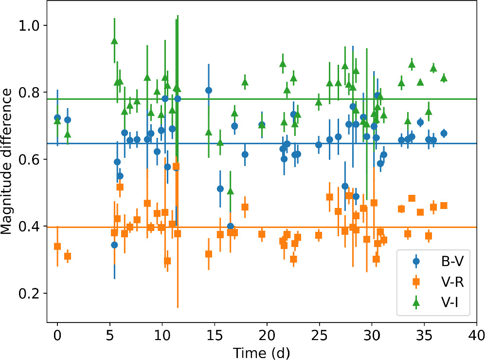
Figure 7. B − V (blue), V − R (orange), and V − I (green) color indices for all 51 epochs obtained with the OWL-Net telescopes. The mean indices are indicated by the blue, orange, and green lines.
Download figure:
Standard image High-resolution image
Figure 8. Reflectance spectrum of OR2 computed using the color indices B − V, V − R, and V − I determined using the OWL-Net observations. The colors are compared with the template spectrum from the Xc (red shaded area) and Xk (blue shaded area) classes.
Download figure:
Standard image High-resolution imageThe X-complex includes asteroids from three distinct classes of objects. All these classes possess similar spectra but can be differentiated based on other properties such as their visual albedo, radar albedo, or circular polarization ratio. These classes are the P, M, and E classes as per the Tholen (1989) taxonomy. They have been absent from taxonomic systems based solely on spectra but have been reintroduced in the newest classification from Mahlke et al. (2021) that takes into account both the spectrum and albedo of an object. In Mahlke et al. (2021), the P type displays an average visual albedo of  , the M type
  , and the E type
  . Based on the albedo determined in this work (see Section 4.1), if we assume that it is an X-type asteroid and thus restrict ourselves to the E, M, and P classes, OR2 would be compatible with an M-type classification.
3.4. Solar Phase Curve
Our photometric observations of OR2 are spanning a large range of solar phase angles. However, the lowest solar phase angle observed during the 2020 apparition was 154, which does not allow us to observe the opposition surge, preventing us from determining the H magnitude. Fortunately, we were able to obtain observations during the 2021 and 2022 apparitions, with solar phase angles ranging from 079 to 1610.
As was pointed out by many authors (e.g., Mahlke et al. 2021; Muinonen et al. 2022), observations obtained during different oppositions can result in different H magnitudes. This is due to the fact that an asteroid observed pole-on (asteroid subobserver latitude of ±90°) will appear larger than an asteroid observed equator-on (asteroid subobserver latitude of 0°). For consistency on the asteroid subobserver observations and on the data set (filter, instrument, method), we are only using the 2021 LDT data, as they contain the lowest observed solar phase angle, for the H magnitude determination here.
Taking into account our shape model of OR2 (see Section 3.6) and its spin axis orientation, these observations were obtained at a mean asteroid subobserver latitude of −47°. This suggests that our determination of the H magnitude will be slightly underestimated compared to an observation performed equator-on. According to the shape model projection at an asteroid subobserver latitude of −47° and at 0°, the mean projected area at −47° is 1.17 times larger than the mean projected area at 0° (averaged over one rotation). This means that our H magnitude will be underestimated by approximately 0.17 mag.
We used an MCMC routine to fit our data set of six observations ranging from 079 to 137 of solar phase angle with data from both pre- and post-opposition. The asteroid subobserver latitude is ranging from −41° to −54°. Our best fit of an H, G model provides H = 15.79 ± 0.04 mag and G = 0.31 ± 0.06.
Using the H, G1, G2 model, we find H = 15.81 ± 0.06 mag, G1 = 0.57 ± 0.22, and G2 = 0.26 ± 0.14. Figure 9 displays the 2021 LDT data (blue circles), the 2022 LDT data (orange circles), and the best H, G model fitted to the 2021 data (blue curve). We can see that a magnitude offset of 0.12–0.19 is present between the 2021 and 2022 data. This offset is due to the fact that the 2022 data were obtained at asteroid subobserver latitudes ranging from −6° to −18°, confirming the expected magnitude offset of 0.13–0.19 estimated based on the shape model cross section at different subobserver latitudes.
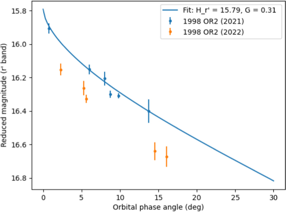
Figure 9. Reduced magnitude as a function of the solar phase angle for the LDT 2021 and 2022 observations (blue and orange circles, respectively). The blue curve corresponds to the best H, G model fit to the 2021 data. An offset of 0.18 mag is noticeable between the 2021 and 2022 data owing to the variation of the asteroid subobserver latitude in between the two apparitions.
Download figure:
Standard image High-resolution imageOur H magnitude determination has been obtained using observations calibrated in the Pan-STARRS  band. However, the International Astronomical Union (IAU) defines the H magnitude in the Johnson V band. We thus have to convert our r' magnitude into a V-band magnitude. We first use the
  relation from Jordi et al. (2006) to convert our result into the Johnson R band. Using the V − R = 0.40 mag obtained in this work, we obtain HR
= 15.60 ± 0.04 mag. Then, we use again the V − R = 0.40 mag color to transform our HR
into HV
= 16.00 ±0.04 mag. However, this H determination is for an asteroid subobserver latitude around 45°. If we apply a magnitude correction of 0.17 ± 0.02, we find HV
= 16.17 ± 0.04 mag. All the uncertainties have been computed using error propagation. It is interesting to note that the MPC is reporting an H magnitude of 16.04, which is compatible with our determination at an asteroid subobserver latitude around 45°. This is mostly due to the fact that the majority of OR2's observations have been obtained at high subobserver latitudes and high solar phase angles. Indeed, low solar phase angles and low asteroid subobserver latitude observations of OR2 can only be obtained when it is far away from Earth and thus when it is too faint for most of the surveys. We also note that the MPC is assuming a G = 0.15 to fit their solar phase curve while we observe a G = 0.31, which significantly departs from their assumptions.
relation from Jordi et al. (2006) to convert our result into the Johnson R band. Using the V − R = 0.40 mag obtained in this work, we obtain HR
= 15.60 ± 0.04 mag. Then, we use again the V − R = 0.40 mag color to transform our HR
into HV
= 16.00 ±0.04 mag. However, this H determination is for an asteroid subobserver latitude around 45°. If we apply a magnitude correction of 0.17 ± 0.02, we find HV
= 16.17 ± 0.04 mag. All the uncertainties have been computed using error propagation. It is interesting to note that the MPC is reporting an H magnitude of 16.04, which is compatible with our determination at an asteroid subobserver latitude around 45°. This is mostly due to the fact that the majority of OR2's observations have been obtained at high subobserver latitudes and high solar phase angles. Indeed, low solar phase angles and low asteroid subobserver latitude observations of OR2 can only be obtained when it is far away from Earth and thus when it is too faint for most of the surveys. We also note that the MPC is assuming a G = 0.15 to fit their solar phase curve while we observe a G = 0.31, which significantly departs from their assumptions.
The values for OR2's G1 and G2 parameters are consistent with the values obtained for M-type asteroids but are also compatible with S-type asteroids, as the photometric phase functions of M and S types are relatively similar (Martikainen et al. 2021).
3.5. Radar CW Bandwidth
We saw earlier that the bandwidth of the CW spectra of OR2 was evolving over time. This evolution is due to the variation of the observation geometry. Such variation of the bandwidth can be used to obtain information on the spin axis orientation.
The bandwidth of a CW spectrum can be modeled using the following relation:

where D is the diameter of the object, P its rotation period, λ the radar wavelength used to perform the observations, and δ the subradar (subobserver) latitude. This model is assuming that the observed object is a sphere, which is a good approximation in the case of OR2. During our observations, the bandwidth was varying from 9.2 to 3.5 Hz between the first and the last day. If OR2 is a perfect sphere, the only variable that can change over time is the angle δ as OR2 is moving on the sky. If we plot the bandwidth of OR2 as a function of the ecliptic coordinates, we notice that it is decreasing linearly. If we were to observe exactly when the spin axis is pointing toward us, we would have a bandwidth of zero. We can thus get an approximation of the pole orientation of OR2 by fitting a line in the 3D space (ecliptic longitude, ecliptic latitude, bandwidth) and extrapolate to the ecliptic longitude and latitude resulting in zero bandwidth. Doing so (see Figure 10), we obtain a pole solution of (1573, −209) or (3373, 209), depending on whether the north or south pole is pointing toward us. We will see (in Section 3.6) that this approximation is very close to the solution found with the full shape modeling inversion. This simple method provides a good approximation of the spin axis orientation only, due to the favorable viewing geometry close to the pole-on view and the motion of OR2 toward a pole-on geometry. Based on the spin axis determined through the full shape modeling, OR2 viewing geometry was only 14° from being pole-on on the last date of radar observations and was 4° away from being pole-on on April 26. Any other observing geometry would have needed a more complex modeling of the bandwidth/ecliptic coordinate variations.
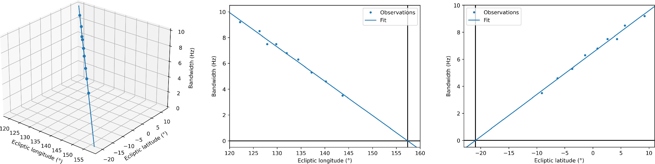
Figure 10. Left panel: fit of a line to the bandwidth observations at a function of the ecliptic longitude and latitude. The extrapolation of the fit is crossing the ecliptic longitude/latitude plane at (1573, −209), corresponding to one solution for the spin axis orientation. Depending on what pole we are observing, a second solution of (3373, 209) is equally likely. Middle panel: same as the left panel, but in a 2D space for the ecliptic longitude only. Right panel: same as the middle panel, but for the ecliptic latitude only.
Download figure:
Standard image High-resolution imageIt is interesting to note that in the case of OR2, we can also use the bandwidth relation to compute its diameter. If we use the solution (1573, −209) for the pole orientation, we find that a mean diameter of 1.85 km is needed to reproduce the observed bandwidth with variation from 1.72 to 1.94 km. These variations are mostly due to the rotation of OR2, which is not a perfect sphere.
3.6. Shape Model
Light-curve and radar data are invaluable to determine the three-dimensional shape of an asteroid. While light-curves can only provide information on the relative dimension of a shape (no information on the absolute size of the shape model) and can only produce convex shapes (Kaasalainen & Torppa 2001; Kaasalainen et al. 2001), radar observations, on the other hand, provide information about the absolute dimensions of the object and constrain the nonconvex features of the shape model.
In most cases, a major difficulty when trying to obtain a unique shape model for an asteroid is to find a unique solution for the spin axis parameters. While using light-curve data only, one needs observations performed at a large number of viewing geometries and over a large range of epochs in order to constrain the sidereal rotation period and the spin axis orientation. In our case, the difficulties encountered in determining the spin axis solution were easier than usual, as we were able to obtain a good first solution for the spin axis orientation using the CW observations.
As a second step, we used the Kaasalainen inversion technique to search for a solution for the convex shape model of OR2 using light-curve observations only. The wide variety of viewing geometries during the 2020 apparition, the use of a couple of light-curves in 2022, and the availability of archived observations, retrieved from the ALCDEF website (Stephens & Warner 2018), obtained in 2009 allowed us to set strong constraints on the spin axis parameters and a shape model. We found a unique solution with a sidereal period of P = 4.1084 ± 0.000 7 hr. A visualization of the obtained shape model is presented in Figure A3 of the Appendix.
For the ecliptic orientation of the spin axis, we find an ecliptic longitude of  and an ecliptic latitude of
  . It is interesting to note that the pole orientation search using light-curve shape modeling is independent of the determination made using radar CW spectra. Here we are finding a unique solution for the pole orientation that is in agreement with the second solution found with radar observations only.
Light-curve shape inversion also usually provides two ambiguous pole solutions like we found for the CW analysis. However, in this case, the observation of the asteroid on an almost pole-on geometry combined with a large variation of the viewing geometry allows to break this uncertainty. Determination of uncertainties on the spin axis parameters when using the Kaasailainen inversion method is not an easy task, as the model does not take into account the uncertainties on the light-curve observations. It is often simply assumed that the uncertainties are of the order of 5°, 10°, or 30° based on the number of data sets and oppositions available (Hanus et al. 2016). Here we are trying to obtain a quantitative estimate of the uncertainties by testing models with fixed spin axis solutions. We are then comparing the residuals on the light-curves between the best shape model and the ones with fixed spin axis. If model residuals deviate by more than 10% from the best shape model, it is considered to be a nonvalid solution; if they deviate by less than 10%, it is considered to be a possible solution. However, this remains a rough estimate of the uncertainties not based on robust statistical analysis.
The last step is to perform the full nonconvex shape modeling inversion using all three data sets (light-curves, radar CW spectra, radar delay-Doppler images). We are using the SHAPE software (Hudson 1994; Magri et al. 2007) to perform the shape modeling inversion using the radar and light-curve data sets. For this step we are using the convex shape model found during the previous step as an initial shape with a pole orientation around (330°, 23°). The best solution that minimizes all three data sets corresponds to a sidereal rotation period of P = 4.10872 ± 0.00001 hr with a spin axis orientation of (3323 ± 5°, 207 ± 5°). The shape possesses dimensions of (2.08 ± 0.10, 1.93 ± 0.10, 1.60 ± 0.03) km. The volume of the shape is V = 3.0 ± 0.5 km3, and its effective diameter is Deff = 1.78 ± 0.10 km. The shape parameters are summarized in Table 6.
Table 6. 1998 OR2 Shape Model Characteristics
| Parameter | Value |
|---|---|
| Maximum dimensions (km) | 2.08 × 1.93 × 1.60 |
| Uncertainties (km) | ±0.10,±0.10,±0.03 |
| Deff (km) | 1.78 ± 0.10 |
| DEEVE (km) | 2.00 × 1.87 × 1.51 |
| Surface area (km2) | 10.67 |
| Volume (km3) | 3.0 ± 0.5 |
| Sidereal rotation period (hr) | 4.108 72 ± 0.00001 |
| Ecliptic pole (λ, β) | (3323 ± 5°, 207 ± 5°) |
Note. The effective diameter (Deff) is the diameter of a sphere with the same volume as the shape model. DEEVE is the dynamically equivalent equal-volume ellipsoid (ellipsoid with the same volume and moment of inertia as the shape model).
Download table as: ASCIITypeset image
As for the shape inversion using light-curves only, it is not easy to estimate uncertainties using the SHAPE software. In the case of SHAPE, the inversion process does take into account the uncertainties on the observations. However, we are here using three types of data sets (i.e., light-curve, radar CW, and radar delay-Doppler). Minimizing all three at the same time is often impossible and often depends on the relative weights that are assigned to the different data sets. Weighting of the different data sets is necessary so that each data set contributes more or less equally to the overall solution. As for the Kaasailainen inversion method, we are trying to obtain quantitative estimates on the uncertainties on the different parameters by testing shape models with different variations of such parameters by fixing them. We then compared the variation of the different χ2, but we are also visually checking the fit of the radar CW spectra and delay-Doppler images. This method is similar to the one used for the determination of the shape model of (1981) Midas (McGlasson et al. 2022) or (101955) Bennu (Nolan et al. 2013). In the case of Bennu, the results from the OSIRIS-REx mission (Lauretta et al. 2019) showed that the shape model was highly accurate with reasonable uncertainties.
Figure 11 shows an example of a CW spectrum obtained on April 21. The blue solid line represents the simulation of the observed CW spectrum represented by the shape model shown in the upper right corner. Figure 12 shows one example per day for delay-Doppler observations. Time is increasing from top to bottom and left to right (the lower left observation comes just before the upper right observation). Figure 13 shows the final shape model from multiple orientation.
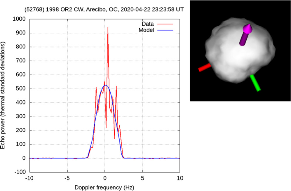
Figure 11. CW spectrum from April 21 (red). The blue solid curve represents the simulation of the observed CW spectrum corresponding to the shape model displayed in the upper right corner.
Download figure:
Standard image High-resolution image
Figure 12. Example of delay-Doppler images for each day of observation of OR2. The leftmost panel shows the observations, the rightmost panel the best shape model as viewed during the observations, and the middle panels represent the modeled delay-Doppler image based on the shape model.
Download figure:
Standard image High-resolution image
Figure 13. Visualization of the shape model of 1998 OR2. The yellow facets represent the parts of the shape that were never observed by radar observations. However, the light-curves are covering the whole surface. The top panel represents the object viewed from the north pole; the middle row represents the shape viewed from the equator at four different longitudes spaced by 90°. The bottom panel represents the shape viewed from the south pole. The large concavity observed in the southern part of the shape model not seen by radar should be taken with caution, as shape modeling using light-curve observations only can only produce convex shape models. However, the combination of radar observations and light-curves obtained at large phase angle allows us to obtain information on concavities even for locations not observed in radar. The crater and large concavities identified in Figures 3 and 4 can be observed close to the green shaft. In the top panel, the crater identified in Figure 3 is visible in the upper right corner and the structure identified in Figure 4 corresponds to the structure around the green shaft.
Download figure:
Standard image High-resolution imageAll the light-curves and the fit to them obtained using the best shape model combining both the radar and the light-curves are presented in Figure A1 of the Appendix. We note that if most of the light-curves are fitted correctly with differences between the model and the observations under the estimated uncertainties, some of the light-curves display large residuals. Comparing these light-curves with other light-curves obtained at similar phase and close in time, we notice that most of the time (when a light-curve displays a misfit) the misfit is due to errors in the light-curves themselves rather than in the shape model. In Figure A1 of the Appendix, we are displaying all the light-curves independently of their quality, and they are all used in the shape modeling, as we noticed that, due to the large number of light-curves and dense time coverage, filtering the light-curves based on their quality was not providing different solutions for the shape model.
3.7. Radar Albedo
The CW spectra combined with a knowledge of the object size provide an estimation of the radar albedo. The radar albedo is defined as the ratio of the projected area of a smooth, metallic sphere (perfect reflector) that would generate the same observed echo power when observed at the same distance to the geometric cross section of the target (see Shepard et al. 2010 for more information on radar albedo).
In the case of OR2, we are measuring a mean radar albedo of 0.29 ± 0.08, when averaged over the nine individual CW observations. The cross section is derived using the best shape model (average radar albedo for each day of observation as listed in Table 4). This value of radar albedo is consistent with the mean radar albedo of X-complex asteroids of 0.28 ± 0.13 as measured by Shepard et al. (2010). However, it is important to note that this mean radar albedo for X-complex asteroids was derived using main-belt objects only and not NEOs.
As we saw earlier, the X-complex is composed of the E, M, and P types. From those, the M types can be distinguished from the E and P types by their high radar albedo. M types have been associated with high content of metal on their surface. Shepard et al. (2010) found that M types have an average radar albedo of 0.41 ± 0.13. With OR2 displaying a radar albedo of 0.29 ± 0.08, it is compatible with an M-type classification but is on the lower end, so other classifications cannot be excluded. We saw previously that Battle et al. (2022) found that the spectrum of OR2 could be explained by an S-type composition with shock-darkened surface or the presence of melts. In a recent study of radar albedos for NEOs, Virkki et al. (2022) found a mean radar albedo for S-type asteroids of 0.19 ± 0.06. Even if based on the mean values of the radar albedo of S- and M-type asteroids, the S-type classification cannot be statistically discarded; we will see later in Section 3.10 that the value of radar albedo found for OR2 implies a near-surface bulk density that is too high for an S-type object.
3.8. Radar Circular Polarization Ratio
We computed the circular polarization ratio (μ c ; ratio between the received SC and OC signals) for the sum of all the CW spectra obtained during each individual observing session (see Table 4). We found a mean μc of 0.291 ± 0.012. μ c can be interpreted as a proxy of the surface roughness. However, Benner et al. (2008) found that μc is correlated with the taxonomic classification of the observed object and thus with composition. In the case of OR2, the μc value is consistent with C-type (0.285 ± 0.12) or S-type (0.270 ± 0.079) asteroids, which would be consistent with the interpreation of Battle et al. (2022).
As already explained, the X-complex is a group containing three distinct compositions, the P, M, and E types. Benner et al. (2008) found that E types are characterized with very high μc above 0.7, thus excluding OR2 from being an E type. The M-type average μc is 0.143 ± 0.055, and that for P type is 0.188 ± 0.019. However, the μc often display large dispersion inside the same taxonomic class. The M types in Shepard et al. (2010) display μc ranging from 0 to 0.37. In Shepard et al. (2010), they break down the M-type (or X-complex) objects into their subclasses in the X-complex. They found that the Xc type has an average μc of 0.26 ± 0.05 (with only a sample of three objects), while the Xk type displays an average μc of 0.13 ± 0.11. The relatively high value for OR2's μc suggests that it is more likely an Xc type rather than an Xk type if we consider that it is an X-complex or M-type asteroid.
3.9. Delay-Doppler Image Polarimetric Map
As with the CW data, delay-Doppler images can be used to obtain information about the polarization of the echo by analyzing the differences between the OC and SC signals. Here we analyze the polarization states of the observed radar echos using the method outlined in Hickson et al. (2021). By recording the states of the OC and SC waves (intensity and phase) at all times, it is possible to derive the Stokes vector and obtain information about the degree of polarization (DP), the degree of linear polarization (DLP), μc , and the m-chi decomposition. More information on these parameters and how to derive them using Arecibo radar observations can be found in Hickson et al. (2021).
We analyzed here the observations of 2020 April 23 when OR2 had the highest signal-to-noise ratio (S/N). This corresponds to the Arecibo observations when OR2 was closest to Earth, but S/N is also higher because OR2 was almost on a pole-on geometry and displayed a smaller bandwidth than during the previous observations. This nearly pole-on geometry decreases the bandwidth and also increases the S/N of each individual frequency channel. To further increase the S/N, all the data collected on that day were stacked together. This results in the stacking of 51 individual observations obtained over 1 hr and 26 minutes. Unfortunately, due to the 4.11 hr rotation period of OR2, such stacking results in smearing of the topographic features observed in the delay-Doppler imaging, as we observed about 35% of the rotation period. Radar polarization mapping requires high S/N, and thus it was impossible to perform analysis on single delay-Doppler images and look for variations of the polarization correlated with topographic features. On the other hand, these maps provide good analysis of the overall scattering properties of OR2.
Figure 14 shows the different polarimetric maps of OR2. The left panel represents the circular polarization ratio (μc ). The middle panel (degree of polarization) represents the fraction of the received echo that is polarized (either circularly or linearly), in contrast to the fraction of the echo that is randomly polarized, or depolarized. Depolarization of the radar signal can result from diffuse scattering from a rough surface or volume scattering within a low-loss medium, among other possibilities. Quasi-specular scattering from smooth structures on the scale of the observing wavelength will result in more strongly polarized radar echos. The right panel represents the m-chi decomposition. The m-chi decomposition is an RGB false-color map using information about the DP (or m) and the ellipticity parameter χ (chi) of the Pointcaré sphere (see Raney et al. 2012; Hickson et al. 2021, for more details). The m-chi RGB map is interpreted as follows (according to Raney et al. 2012): blue indicates an odd number of bounces or mostly single quasi-specular reflection, red indicates an even number of bounces or mainly double-bounce quasi-specular reflection, and green indicates light that has been depolarized.
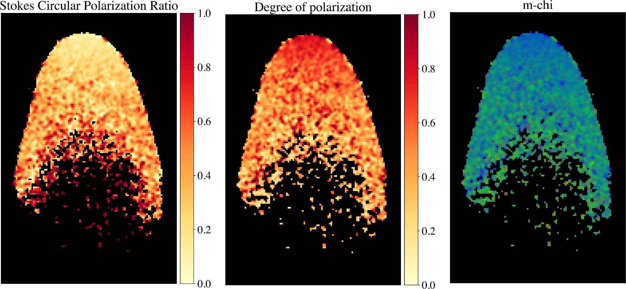
Figure 14. Radar polarization images of 1998 OR2. The panels from left to right represent the circular polarization ratio, the degree of linear polarization, and the m-chi decomposition.
Download figure:
Standard image High-resolution imageIn the case of OR2, the μc map shows a low value of the circular polarization (light color; μc of 0.1–0.2) around the leading edge and slowly increasing values as we move toward the trailing edge. For high incidence angle, we are observing higher values of the μc as expected for a surface covered in regolith. Indeed, the incidence angle is minimum around the leading edge and thus corresponds to quasi-specular backscattering dominating, whereas diffuse scattering begins to dominate as the incidence angle increases. On the other hand, a surface covered with boulders, as on Bennu (Lauretta et al. 2019), will result in more random scattering angles all over the surface that depend on the boulder shape and electric properties and not on the location on the surface (leading or trailing edge). The electric permittivity of Bennu's regolith is lower than that of OR2's regolith based on their radar albedos, which also plays a role in the radar scattering, because regolith with a greater electric permittivity reflects and refracts light more effectively. Thus, Hickson et al. (2021) are seeing a more homogeneous μc map in the case of Bennu. The reason that the μc is increasing for increasing diffuse scattering is because the diffuse scattering acts as a randomization of the circular polarization orientation and the depolarization of the light (fully depolarized light would have a μc of 1). This depolarization effect can be seen on the degree of polarization map, where the polarization is high (around 0.9–1 and colored in red) and is decreasing with incidence angle. The anticorrelation between the μc and the DP shows that the μc is due to depolarization of the light instead of double-bounce scattering that would enhance especially the SC signal. In this case, the depolarized light contributes equally to the SC and OC signal and thus results in an increase of the μc . We can also see this effect in the m-chi decomposition map (right panel), where the blue and and green dominate, while the red, which indicates double-bounce scattering, is absent from the map. The incidence angle dependence and anticorrelation between μc and DP of the polarimetric maps of OR2 suggest that it is most probably covered with a deep layer of regolith. On the other hand, the fact that the average value of the μc is higher compared to other M-type asteroids also suggests that OR2 should still possess some decimeter-scale surface roughness.
3.10. Near-surface Bulk Density
Radar observations can be used to derive the near-surface bulk density (ρbd) using information about the radar albedo of the observed target. Radar albedo is correlated to the density of the refracting surface down to depths of about ∼1 m. There exist several relations in the literature that try to link the radar albedo to the bulk density. Making use of the one presented in Shepard et al. (2010), we derive a bulk density ρbd = 3.1 ±0.7 g cm−3.
In our cases, we have more information about our target than just the radar albedo. Using the shape model of OR2 derived in this work and the delay-Doppler observations, we can obtain information about the scattering properties of the near surface. The best shape model was obtained using the so-called radar scattering cosine law (Mitchell et al. 1996). This scattering equation is represented by two parameters R and C and is written as follows:

In this equation, A represents a small area of the surface, θ is the scattering angle, R is the Fresnel reflectivity at normal incidence, and C is related to the rms slope angle (in other words, the larger C is, the more specular scattering is present). The C parameter is fitted during the shape modeling process. The shape modeling software is optimizing this parameter to find the one that provides the best fit to the observations. On the other hand, the R parameter cannot be optimized by the shape modeling software. It is usually set to a reasonable value and is fixed during the shape modeling process. We are thus determining it a posteriori using the final shape model, computing the scattering contribution of each element, and finding the R value that best models the observed cross sections and radar albedos. The best shape model fit to the radar data provides C of 1.16 and 0.42 and R of 0.21 and 0.067 for the OC and SC observations, respectively.
Hickson et al. (2018) suggested that the near-surface bulk density could be derived from the electric permittivity ( ) so that ρbd = 3.257(1/3 − 1). Using R and assuming the same relative uncertainties that the radar albedo has, we derived a relative electric permittivity of
  that corresponds to a near-surface bulk density of ρbd = 3.0 ± 0.7 g cm−3, which is consistent with the previous determination obtained using a model based on the radar albedo only.
The mean near-surface bulk density that we derived here would be consistent with a 10% porosity if we consider OR2 being composed of pure S-type-like material (see Consolmagno et al. 2008 for estimation of the grain density for different ordinary chondrites materials). If we consider OR2 being composed of pure FeNi material, its porosity should be around 60%. A 50%/50% mixture of FeNi and silicate (which would still be considered as a metal-rich asteroid) would require a 50% porosity.
3.11. Thermophysical Modeling
OR2 was observed by the NEOWISE spacecraft at two distinct epochs on 2020 March 18 and 2020 April 25. During these two epochs, OR2 was observed in both the W1 (3.4 μm) and W2 (4.6 μm) bands. According to the shape model best solution for the spin axis orientation, these two observations have been performed at highly different viewing geometries. The first epoch (March) was obtained at a solar phase angle of 59° and when OR2 was viewed on an equator-on (subobserver latitude of 30°) geometry with the Sun at a pole-on geometry (sub-Sun latitude of 60°). During the second epoch, the solar phase angle was close to the first epoch with 65°; however, it was observed on a pole-on geometry for the observer (subobserver latitude of 74°) and with the Sun on an equator-on geometry (sub-Sun latitude of 30°). NEOWISE observations can be used to determine the diameter and albedo of the observed target (Mainzer et al. 2011). Here we first make use of the NEATM model (Harris 1998) on the two NEOWISE epochs, which results in a diameter of 1.93 ± 0.31 km. This result is consistent with the diameter determination with other techniques. Using an H magnitude of 16.17 ± 0.04 (the NEOWISE observations were obtained when OR2 was observed at high subobserver latitude), we find an albedo of pV = 0.19 ± 0.06, consistent with other albedo determinations.
Previously, the albedo and diameter of OR2 were determined by Masiero et al. (2021) using one of these epochs of the NEOWISE data. In that work they find a diameter of D = 2.51 ± 0.81 km and an albedo of  . The Masiero et al. (2021) fit for OR2 used a different H magnitude (H = 16.0 vs. H = 16.17 here) and a slightly different assumed beaming value (η = 1.4 vs. η = 1.2 here), which is responsible for the offset from the results found here. The NEOWISE-derived fits we present are consistent with those published by Masiero et al. (2021) within the 1σ uncertainties. These uncertainties are derived from Monte Carlo simulations of the input data and assumed parameters. This emphasizes how minor alterations in assumed beaming or changes in H magnitude can significantly impact the results of NEATM fitting.
Second, we used the individual observations, obtained during the first epoch, to perform a more detailed thermophysical modeling (TPM) of OR2. Indeed, during the first epoch, the NEOWISE observations covered multiple rotations of OR2 and yielded a well-characterized thermal light-curve (see Figure 15). We used the detailed nonconvex shape model derived in this work and a TPM to estimate the emitted thermal flux of OR2 according to the approach of MacLennan & Emery (2022). The TPM used one-dimensional heat transfer and accounted for self-shadowing/heating effects to calculate surface temperatures for a bolometric Bond albedo of A = 0.06. Surface roughness is explicitly accounted for by using spherical section craters with different opening angles (MacLennan & Emery 2019). Various combinations of half-opening angle (γc
) and fraction of area covered by the craters (fR
) are used to adjust the overall degree of roughness, encapsulated by the mean surface slope ( see Table 7). Furthermore, we incorporated reflected sunlight and scaled the flux for each wavelength according to the spectrum of the Sun and the apparent brightness of OR2. These modeled (thermal + reflected) fluxes were compared to the thermal light-curve of OR2. For each thermal light-curve the shape model was fixed and the size was allowed to vary according to the uncertainties of the radar shape model. On the other hand, the thermal inertia and surface roughness were allowed to vary to best match the observations to calculate the reduced minimum χ2 goodness of fit (χ2).

Figure 15. Results of the TPM on the two NEOWISE light-curves obtained in two bands, W1 and W2, during the first epoch of observations. Left panel: χ2 of the TPM fit as a function of thermal inertia and surface roughtness. Varying the surface roughness leads to almost identical χ2, but result in a significant variation of the thermal inertia. Middle panel: best fit of the TPM on the W1 NEOWISE light-curve. Right panel: same as the middle panel, but for the W2 band.
Download figure:
Standard image High-resolution imageTable 7. Default TPM Surface Roughness Values
| Name | γc | fR |

|
|---|---|---|---|
| Smooth | ⋯ | ⋯ | 0° |
| Minor | 45° | 0.4 | 65 |
| Low | 45° | 0.5 | 107 |
| Intermediate | 45° | 0.6 | 169 |
| Medium | 68° | 0.7 | 235 |
| Considerable | 68° | 0.8 | 301 |
| High | 90° | 0.6 | 438 |
| Maximum | 90° | 1.0 | 579 |
Notes.
γc
: the crater helf-opening angle; fR
: fraction of surface covered by craters;  : mean surface slope (Hapke 1984; MacLennan & Emery 2019).
Download table as: ASCIITypeset image
Initially, we made an assumption of equal spectral emissivity for W1 and W2 of 0.9, for which it was difficult to simultaneously fit both W1 and W2 light-curves. We find that lowering the W2 emissivity yielded much better fits, as discussed below. Particularly, we used a W1 spectral emissivity of 0.88, 0.90, and 0.92, which was paired with different emissivities of 0.82, 0.85, 0.88, and 0.90 for the W2 band. Given our modeling results, we find it highly probable that the spectral emissivity of OR2 is lower in the W2 bandpass than in the W1 bandpass. We prefer the solutions using considerable roughness, as they are more consistent with the radar-derived size of OR2 and moderate roughness indicated by the radar CPR. More extreme W2 spectral emissivities were required to fit the data using lower roughness values, but they still cannot be ruled out by thermal photometry. Spectral observations using the James Webb Space Telescope, for example, would be needed to confirm this.
The TPM modeling fits are consistent with the size as constrained by radar observations. We varied the size within the acceptable 1σ margin of uncertainty (1.7–1.9 km) in order to properly assess the uncertainties in the other model parameters. Because of the uncertainty in roughness and spectral emissivity, the thermal inertia is only constrained to <250 J K−1 m−2 s−1/2. The insensitivity to surface roughness is most likely due to the high phase angle and equator-on geometry of the NEOWISE observations (Rozitis 2017). We found that different roughness values correlate with the best-fit thermal inertia, as seen by the differently colored points in Figure 15: larger roughness corresponding to higher thermal inertia except for the two highest default roughness parameters. Interestingly, these two scenarios used a hemispherical crater, rather than a spherical crater with smaller γc (Table 7). Investigating this phenomenon is beyond the scope of this paper, but we suspect that it is an artifact related to the high phase angle and extreme opening angle of the hemispherical (γc = 90°) crater.
3.12. Radar Astrometry
Since we know OR2's dimensions from the shape model, we can determine the position of its center of mass (COM) relative to the leading edges seen in the delay-Doppler images. Using the shape model gives more accurate astrometry than what we could obtain from visual inspection during the radar observations. Table 8 gives the final delay measurements. We are only reporting delay measurements because Doppler measurements would add little in comparison.
Table 8. Astrometric Measurements of 1998 OR2's Center of Mass from Arecibo, Using the Shape Model
| Date | Time (UT) | Measurement (s) | Uncertainty (μs) |
|---|---|---|---|
| 2020 Apr 16 | 23:39:00 | 74.169 888 28 | 0.55 |
| 2020 Apr 17 | 00:39:00 | 74.006 133 30 | 0.55 |
| 2020 Apr 17 | 23:49:00 | 70.213 370 86 | 0.54 |
| 2020 Apr 18 | 23:37:00 | 66.419 421 12 | 0.54 |
| 2020 Apr 19 | 23:42:00 | 62.708 392 59 | 0.54 |
| 2020 Apr 22 | 00:23:00 | 55.726 484 71 | 0.53 |
| 2020 Apr 23 | 00:30:00 | 52.603 664 00 | 0.53 |
| 2020 Apr 23 | 23:47:00 | 49.859 572 30 | 0.53 |
Note. The measurement reference point for Arecibo is the center of curvature of the dish. The uncertainties come from two terms added in quadrature: 0.5 μs (minimum systematic uncertainty of any delay measurement from Arecibo with a baud length of 0.5 μs or less), and the uncertainty in OR2's delay depth (which depends on its orientation at each time).
Download table as: ASCIITypeset image
Three round-trip delay measurements, with uncertainties ranging from 1.2 to 8 μs, were used to produce JPL Horizon orbit solution #280 30 shortly after the track in 2020. Analysis in support of a stellar occultation visible from southeastern Australia on May 19 (subsequently rained out) found that the measurements debiased the pre-radar trajectory solution by 2 km and reduced the plane-of-sky uncertainty ellipse area from 2.05 to 0.05 arcseconds2, a −97.6% decrease (Figure 16). They increased the predictability of future Earth encounters by 447 yr.
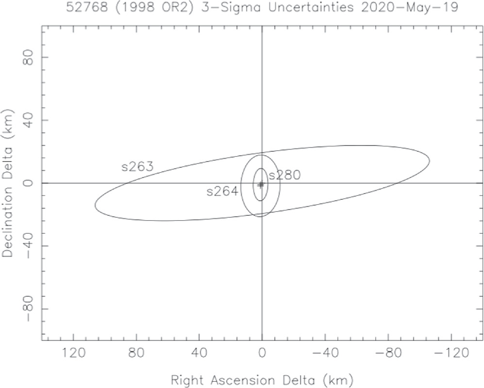
Figure 16. Plane-of-sky position and uncertainty for OR2 on 2020 May 19 for JPL Horizon orbit solutions #263 (pre-radar observations), #264 (including the first two radar delay measurements), and #280 (including the third radar measurement).
Download figure:
Standard image High-resolution imageThese measurements are here replaced by eight refined measurements reduced relative to the shape-derived COM. The new reductions have much smaller uncertainties in the range 0.53−0.55 μs and extend the radar data arc from 5.1 to 7 days. This refined astrometry was used along with the current optical data set to produce JPL Horizon orbit solution #346.
Comparison with the prior solution #345 finds a mean reduction in the uncertainty of the six classical orbital elements of −10.2% at the solution epoch owing to inclusion of the shape-reduced astrometry. The Earth encounter predictability window, a coarse metric of interest (defined as the time span over which Earth encounters less than 0.1 au can be predicted with 3σ uncertainties less than ± 0.1 au in distance and ± 10 days in time), is unchanged at AD 1168–3039 for this extensively measured multi-apparition object. The new measurements are available from the radar astrometry database. 31
4. Discussions
In the previous sections, we presented the results obtained using each individual datum or technique. Each of these data sets or techniques have their strengths and type of physical characterization information they provide. In this section, we will discuss the individual parameters and physical properties of OR2 by combining the different results.
4.1. Size and Albedo
Several independent techniques can be used to derive the size and albedo of an asteroid. Each individual technique provides information on either the size or the albedo, and both can be linked using the  relation that links the diameter (in kilometers), the albedo, and the H magnitude in the V band of an asteroid (Bowell et al. 1989). In the case of OR2, we found that the H magnitude is H = 16.00 ± 0.04 during the 2021 apparition. This corresponds to the H magnitude when the asteroid is observed at a subobserver latitude of 45°. Taking into account the shape model derived in this work, we find that the average equivalent diameter over one full rotation is 1.87 ± 0.10 km when observed at a subobserver latitude of 45°. Using the relation linking the albedo to the diameter and the H magnitude, we find that OR2 has an albedo of 0.20 ± 0.02.
In the case of radar observations, we are measuring the diameter and convert it to albedo using the H magnitude. However, we also obtained an albedo determination using polarimetric observations. In that case we found an albedo of  . This determination is consistent with the one obtained with radar. Assuming an equivalent diameter of 1.74 ± 0.1 km (mean diameter when OR2 is observed equator-on), we find an equator-on H magnitude of 16.03 ± 0.19, which is consistent with the photometric observations. We again stress here that we did not observe OR2 in polarimetry at phase angles lower than the inversion angle. Thus, the albedo obtained using polarimetry only should be taken cautiously.
Finally, the thermal observation from NEOWISE provided a diameter of 1.93 ± 0.31 km and an albedo of pV = 0.19 ± 0.06.
We have obtained three independent determinations of the albedo; the weighted average provides pV = 0.21 ± 0.02. In the case of the diameter, we find an average value of D =1.80 ± 0.10 km.
4.2. Surface Roughness
The recent visits of spacecraft to asteroids Bennu and Ryugu by OSIRIS-REx and Hayabusa 2, respectively, showed surfaces covered in boulders and almost devoid of fine regolith as was observed for other asteroids like Itakowa by Hayabusa. These observations were striking, as it had been hypothesized that Bennu had a smooth surface based on radar μc (Nolan et al. 2013) and thermal inertia (Emery et al. 2014) measurements. On the other hand, the radar polarimetry analysis performed by Hickson et al. (2018) is suggesting a surface covered in boulders instead of fine regolith.
As for Bennu, we also have radar, polarimetric, and thermal observations for OR2. As was already discussed in Section 3.9, the radar polarimetric map of OR2 is different from the one of Bennu. For OR2, we are observing higher μc for larger incidence angle that is correlated with a decrease of the DP for larger incidence angles too. In thermal observations we saw in Section 3.11 that to keep the size of OR2 to reasonable values, the TPM analysis leads to low thermal inertia, which is characteristic of a deep pool of fine regolith, while higher thermal inertia is more indicative of boulders. If we were not able to obtain a consistent value of the thermal inertia, we can assume that it is relatively low, thus suggesting that the surface of OR2 is mainly covered by a deep pool of regolith. On the other hand, the relatively large mean value of the μc indicates that OR2 still possesses some decimeter-scale near-surface roughness.
4.3. Surface Heterogeneities
We saw in Section 3.1 that the optical polarization of OR2 is varying as a function of rotation phase. As optical polarization is independent of the shape of the target, these variations should be related to variations of the surface properties. Figure 17 shows the orientation of the shape model corresponding to the maximum of polarization (top row), average polarization (middle row), and minimum polarization (bottom row). We notice again that the shape model was observed at an almost pole-on geometry; hence, most of the northern hemisphere of OR2 is always illuminated and seen during the observations. This implies that the features resulting in the polarimetric variation are most probably located near the equator of OR2, which is the only region that is going through day/night cycles.

Figure 17. Orientation of the OR2 shape model when it was observed in polarimetry. The top row corresponds to the maximum of polarization, the bottom row corresponds to the minimum of polarization, and the middle row corresponds to the transition from the maximum to the minimum of polarization. Each column represents an individual observation night. The observation date and the aspect angle (angle between the line of sight and the spin axis) are displayed on top of each column. The model is only displayed when we observed at that specific time and orientation.
Download figure:
Standard image High-resolution imageThe thermal light-curve from NEOWISE also suggests that the surface of OR2 is heterogeneous, as our model failed to properly model it using homogeneous surface properties values. Highly different values of the emissivity, size, and thermal inertia provide similarly good fits based on the χ2 value, but with very different shapes of the light-curve. To properly model the light-curves, we would probably need to assign different properties to different parts of the model, but this is beyond the capabilities of the fitting routine that we are currently using.
OR2's shape model displays interesting features as we discussed previously. If we pay attention to the first row of Figure 17, which represents the orientation of the shape with respect to the observer when the polarization is maximum, we note that the shape is almost devoid of concavities and appears relatively smooth with a nicely defined equatorial ridge. On the other hand, when we transition toward the minimum of polarization from the middle row to the third row, we see that the shape model displays more and more concavities. On the bottom row, when the polarization is minimum, the equator looks truncated by a large concavity, and thus we are almost not seeing any equatorial region. If the variation of polarization is indeed related to how much of the equatorial region is seen or the concavities seen around the equatorial region, we could interpret the variation of polarimetry as a difference in surface properties for the equatorial ridge and the rest of the surface. When most of the equatorial ridge is seen, the polarization is high (low albedo or larger grain size), whereas when we see less of the ridge, the polarization is low (high albedo or smaller grain size). We could also interpret the variation as due to the presence of the concavities themselves, which could be related to impacts. The concavities would be linked to lower polarization and thus higher albedo or smaller grain sizes.
5. Conclusions
We observed the near-Earth asteroid 1998 OR2 in photometry, polarimetry, and radar during its 2020 close flyby. Additional photometric observations were obtained during its 2021 and 2022 apparitions to obtain observations at low solar phase angles and to improve the shape modeling.
Using the photometric observations, we obtain a new photometric solar phase curve for 1998 OR2 that allowed us to determine its absolute H magnitude. We find in this work an H of 16.17 mag for an equator-on viewing geometry with a G = 0.31 ± 0.06 or G1 = 0.57 ± 0.22 and G2 = 0.26 ± 0.14. This new determination for the H magnitude is slightly higher than the one obtained from the MPC, but 1998 OR2 can almost never be observed on an equator-on geometry, leading to a slightly lower H determination when observed at high subobserver latitude. Using the shape model derived in this work, we were able to correct for that effect.
We also used the photometric observations to obtain the colors of 1998 OR2 and found color indices of B − V = 0.65 ± 0.01 mag, V − R = 0.40 ± 0.01 mag, and V − I = 0.78 ± 0.01 mag. Using those color indices, we find that the best taxonomic classification for 1998 OR2 is of Xk or Xc type. Combined with information obtained from radar and about OR2's albedo, if OR2 is an X-complex asteroid, we can narrow down its taxonomic classification to the M type.
Using the combined observations in radar and photometric light-curves, we derived a unique nonconvex shape model for 1998 OR2. The shape model shows a top-shape-like asteroid with an equatorial ridge, similar to asteroids Bennu, Moshup, and Didymos. The shape model also presents large concavities and craters that are mostly located on one side of 1998 OR2. Indeed, one side looks like a regular top-shape asteroid with an equatorial ridge, while the other side seems to have been truncated with the presence of a crater that was clearly identified in the leading edge of the delay-Doppler observations. We find that 1998 OR2 possesses a sidereal period of P = 4.10872 ± 0.00001 hr and a pole orientation of (3323 ± 5°, 207 ± 5°). The shape has dimension of (2.08 ± 0.10, 1.93 ± 0.10, 1.60 ± 0.03) km with a volume of V = 3.0 ± 0.5 km3, corresponding to an equivalent diameter of 1.80 ± 0.10 km.
The polarimetric observations show that 1998 OR2 is displaying polarization variations that are correlated with its rotation phase. These variations have been measured to be 5.5% relative to the mean polarization. These variations suggest that 1998 OR2 possesses a heterogeneous surface that can be linked to either the equatorial ridge (the ridge would possess different surface properties compared to the polar regions) or the cratered versus undisturbed side.
We also derived the albedo for 1998 OR2 independently using the different observation techniques used in this work. The radar shape model combined with our new H magnitude determination provides an albedo of pV
= 0.20 ± 0.02. Using polarimetric observations, we find an albedo of  . Using archived observations from the NEOWISE satellite, we find an albedo of pV
= 0.19 ± 0.06. Combining all these albedo determinations, we find that 1998 OR2 should possess an albedo of pV
= 0.21 ± 0.02.
. Using archived observations from the NEOWISE satellite, we find an albedo of pV
= 0.19 ± 0.06. Combining all these albedo determinations, we find that 1998 OR2 should possess an albedo of pV
= 0.21 ± 0.02.
Using the shape model derived in this work and the CW radar observations, we derived a radar albedo for 1998 OR2 of 0.29 ± 0.08. Using the radar albedo and the radar scattering properties of the surface of 1998 OR2, we determine that the near-surface bulk density of 1998 OR2 is ρbd = 3.1 ± 0.7 g cm−3. Such density is hardly compatible with a pure silicaceous surface, and at least some metalic content should be present on the surface of 1998 OR2 to explain its high radar albedo and surface bulk density.
In conclusion, we find that OR2 is probably not an S-type asteroid but more likely an M-type asteroid. M-type asteroids can be diverse, and there is still no consensus on a unique interpretation to explain their surface properties. They have long been thought to be the metallic core of differentiated bodies, but over the years other interpretations, including the mixture of silicates and metal, have been proposed. The fact that we could have considered an S-type classification for OR2 shows that interpreting its surface composition as either metallic or siliceous is erroneous, and it is most probably a mixture of the two. This mixture induces heterogeneities on its surface that can be seen in polarimetry and thermal infrared.
Based on all the physical properties obtained in this work, we find that 1998 OR2 possesses similar characteristics to M-type asteroids, which makes 1998 OR2, with a Δv of only 6.5 km s −1, a very interesting target for future space missions. Understanding the properties of metallic objects and their abundance in the near-Earth environment is of first importance for planetary defense to prepare mitigation strategies in the case of the discovery of an X/M-type asteroid in a collision trajectory with Earth.
Acknowledgments
M.D. and M.F. acknowledge the NASA Yearly Opportunity for Research in Planetary Defense (YORPD) grant No. 80NSSC22K0237 "Polarimetry as a tool for physical characterization of potentially hazardous asteroid."
The Arecibo planetary radar observations were fully supported by the National Aeronautics and Space Administration's (NASA's) Near-Earth Object Observations program through grant No. 80NSSC19K0523 awarded to the University of Central Florida (UCF).
The Torino polarimeter was built at the INAF—Torino Astrophysical Observatory and funded by INAF in the framework of INAF PRIN 2009. Part of the polarimetric data in this work have been obtained on the C2PU facility (Calern Observatory, O.C.A.). TRAPPIST is a project funded by the Belgian Fonds (National) de la Recherche Scientifique (F.R.S.-FNRS) under grant PDR T.0120.21. TRAPPIST-North is a project funded by the University of Liège, in collaboration with the Cadi Ayyad University of Marrakech (Morocco). E.J. is an FNRS Senior Research Associate. M.H. thanks the Slovak Academy of Sciences (VEGA No. 2/0059/22) and the Slovak Research and Development Agency under contract No. APVV-19-0072. This article includes observations made with the TAR2 telescope operated on the island of Tenerife by the Instituto de Astrofísica de Canarias in the Spanish Observatorio del Teide.
A.C., J.L., and H.M. acknowledge support from the ESA NEOROCKS (Near Earth Objects Rapid Observation, Characterization and Key Simulations) project, funded by the European Union's Horizon 2020 research and innovation program under grant agreement No. 870403.
This paper was partially based on observations obtained at the Optical Wide-field patroL Network (OWL-Net), which is operated by the Korea Astronomy and Space Science Institute (KASI).
H.M. and J.L. acknowledge support from the ACIISI, Consejería de Economía, Conocimiento y Empleo del Gobierno de Canarias and the European Regional Development Fund (ERDF) under grant with reference ProID2021010134. D.M., F.T.R., and J.L. acknowledge support from the Agencia Estatal de Investigacion del Ministerio de Ciencia e Ińnovacion (AEI-MCINN) under grant "Hydrated Minerals and Organic Compounds in Primitive Asteroids" with reference PID2020-120464GB-100.
This work uses data obtained from the Asteroid Lightcurve Data Exchange Format (ALCDEF) database, which is supported by funding from NASA grant 80NSSC18K0851.
This work made use of the NASA JPL Horizons ephemeris service available at https://ssd.jpl.nasa.gov/horizons/
Appendix
The shape model fit to the photometric light-curves is presented in Figure Set A1. The shape model fit to the delay-Doppler data is presented in Figure Set A2. The convex shape model obtained with light-curves only is presented in Figure A3.
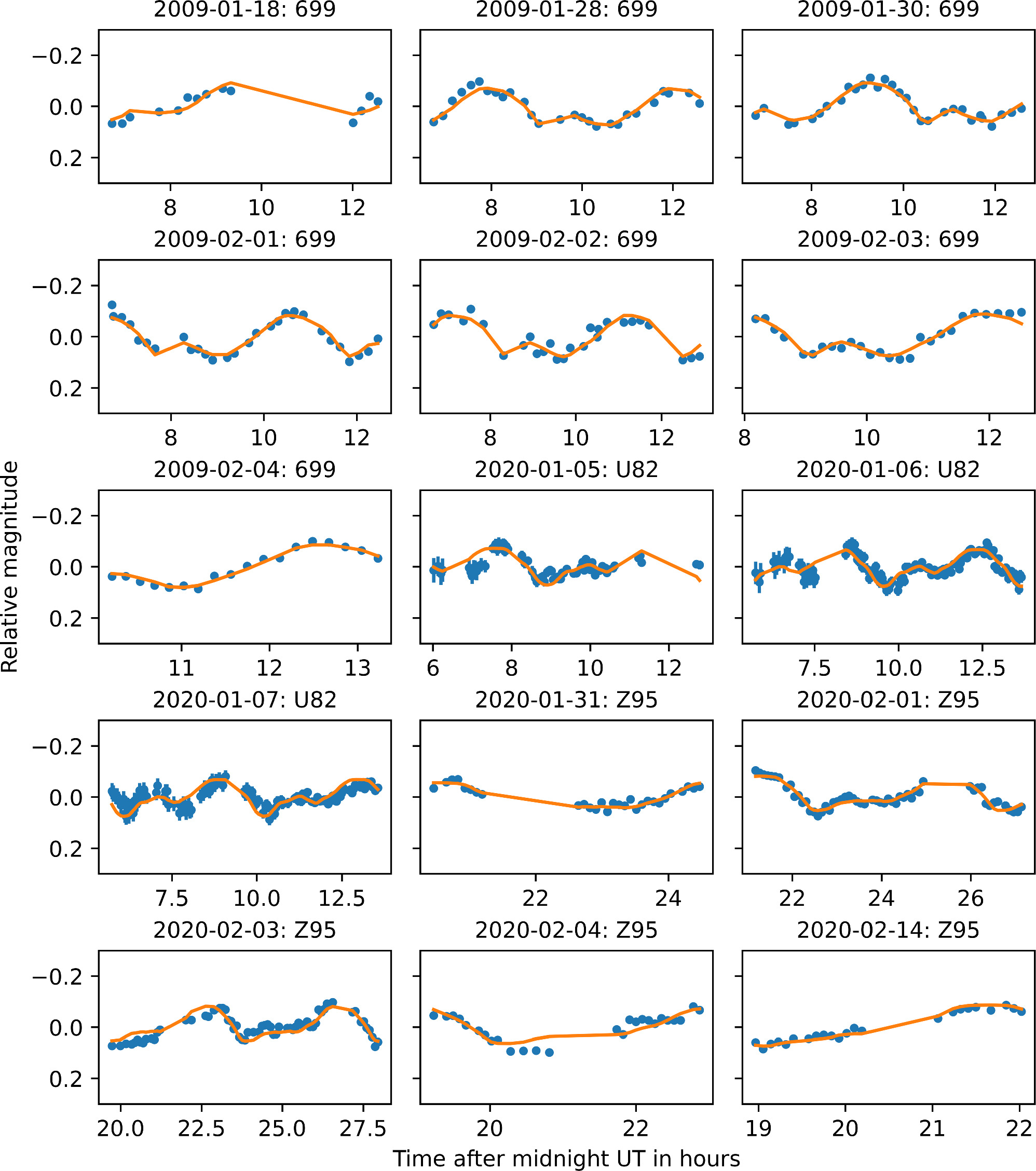
Figure A1.
Photometric light-curves of OR2 used for the shape model. The observations are represented with blue circles (the markers are usually larger than the error bars). The synthetic light-curves using the best shape model are displayed as an orange line on the observed data. (The complete figure set (5 images) is available.)
Download figure:
Standard image High-resolution image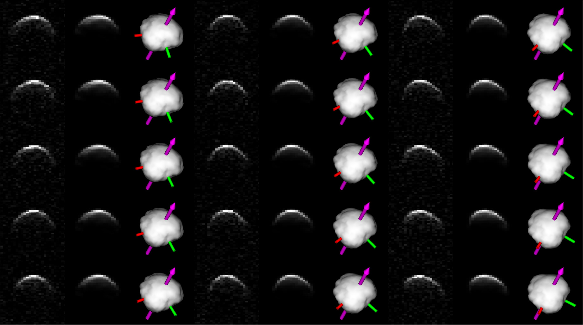
Figure A2.
1998 OR2 delay-Doppler observations of 2020 April 16 and shape model fit. Images are displayed in columns with time increase from top to bottom and left to right. The resolution is 75 m pixel–1 in range (y-axis) and 0.47 Hz in frequency (x-axis). (The complete figure set (16 images) is available.)
Download figure:
Standard image High-resolution image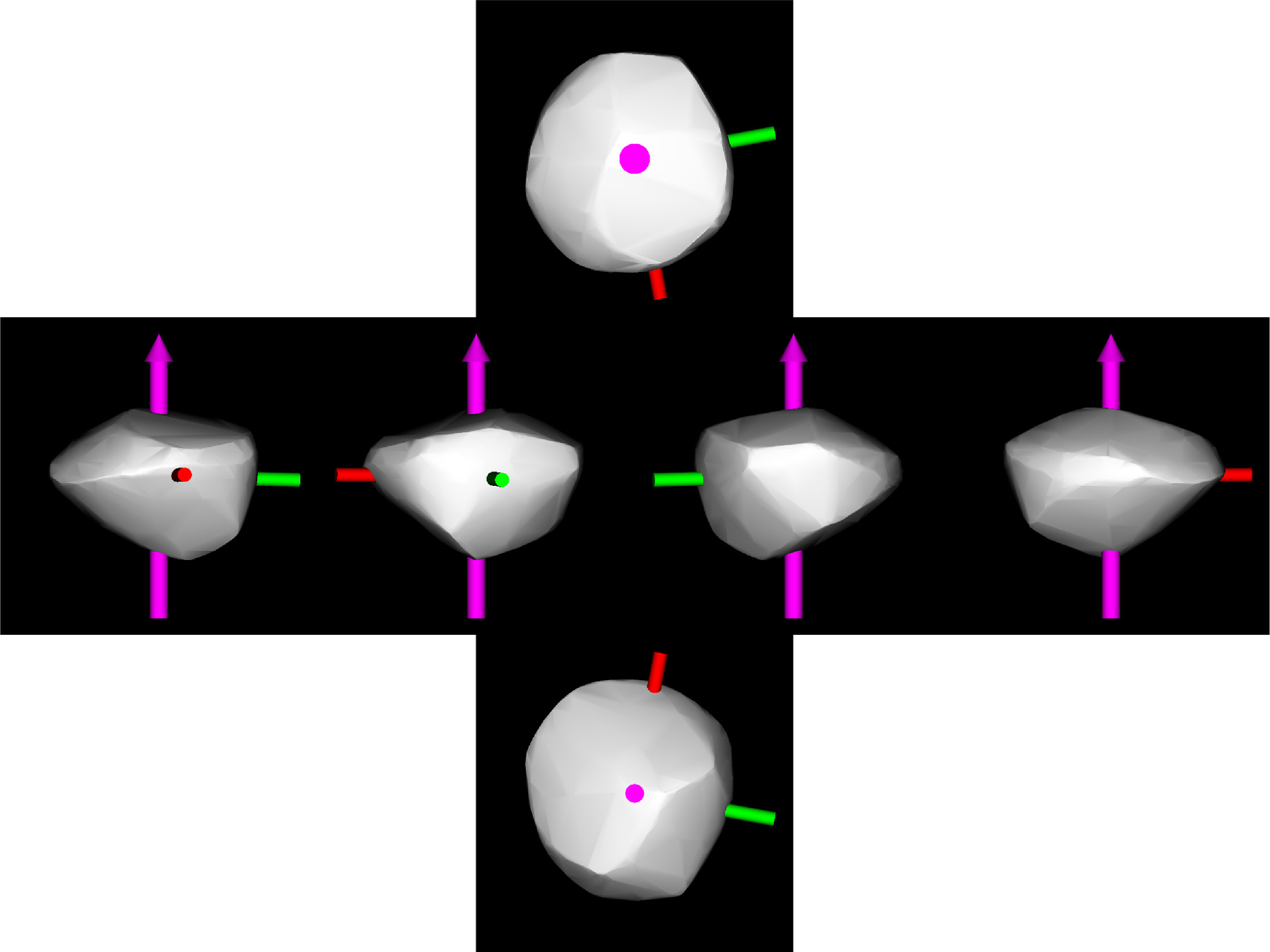
Figure A3. Visualization of the convex shape of 1998 OR2 obtained using light-curves only and the Kaasalainen inversion method. This shape has been used as the initial shape for the light-curve+radar nonconvex shape modeling. The top panel represents the object viewed from the north pole. The middle row represents the shape viewed from the equator on four different longitudes spaced by 90°. The bottom panel represents the shape viewed from the south pole.
Download figure:
Standard image High-resolution image
Footnotes
- 28
- 29
- 30
- 31