


1 Introduction
Generalized geometry was proposed by Hitchin [Reference HitchinH] as a framework unifying complex and symplectic structures. The two latter can be viewed as particular instances of the notion of a generalized complex structure, the theory of which was developed in [Reference GualtieriGu1, Reference GualtieriGu2] including a geometrization of Barannikov’s and Kontsevich’s extended deformation theory.
Similarly, pseudo-Riemannian metrics have a fruitful counterpart in generalized geometry, which can be used, for instance, to unify and geometrize the structures involved in type II supergravity [Reference Coimbra, Strickland-Constable and WaldramCSW]. A generalized pseudo-Riemannian metric together with a divergence operator is indeed sufficient to define a notion of generalized Ricci curvature and thus to pose a generalized Einstein equation as the vanishing of the generalized Ricci curvature [Reference García Fernández and StreetsGSt]. In the context of supergravity and string theory, the divergence operator is related to the dilaton field, which is itself subject to a field equation.
A generalized geometry formulation of minimal six-dimensional supergravity has been given in [Reference García Fernández and ShahbaziGS] with a particular case of the generalized Einstein equation as the main bosonic equation of motion. It would be interesting to classify left-invariant solutions on six-dimensional Lie groups using the theory developed in our present work. We note that by taking, for instance, the product of a pair of three-dimensional generalized Einstein Lie groups (as defined below in the introduction and classified in our paper), we obtain a six-dimensional generalized Einstein Lie group. If one imposes, in addition, a self-duality condition on the three-form, one arrives at (decomposable) solutions of the equation of motion mentioned above. Other (indecomposable) solutions on products of three-dimensional Lie groups have been constructed in [Reference Murcia and ShahbaziMS]. Examples of invariant Ricci-flat Bismut connections on compact homogeneous Riemannian manifolds have been constructed in [Reference García Fernández and StreetsGSt, Reference Podestà and RafferoPR1, Reference Podestà and RafferoPR2]. They include non-Bismut-flat examples [Reference Podestà and RafferoPR1, Reference Podestà and RafferoPR2] and give rise to invariant positive definite solutions of the generalized Einstein equation with Riemannian divergence operator.
In this paper, we focus on left-invariant generalized pseudo-Riemannian metrics on Lie groups G. We develop the theory on arbitrary Lie groups in Section 2 and, based on that theory, provide a complete classification of left-invariant solutions of the generalized Einstein equation on three-dimensional Lie groups in Section 3.
First, we show in Proposition 2.4 that, up to an isomorphism, the generalized metric
 $\mathcal {G}$
and the Courant algebroid structure are encoded in a pair
$\mathcal {G}$
and the Courant algebroid structure are encoded in a pair
 $(g,H)$
consisting of a left-invariant pseudo-Riemannian metric g and a left-invariant closed three-form H on G. Then we describe the space of left-invariant torsion-free and metric generalized connections D on
$(g,H)$
consisting of a left-invariant pseudo-Riemannian metric g and a left-invariant closed three-form H on G. Then we describe the space of left-invariant torsion-free and metric generalized connections D on
 $(G,\mathcal {G}_g,H)$
as a finite-dimensional affine space modeled on the generalized first prolongation of
$(G,\mathcal {G}_g,H)$
as a finite-dimensional affine space modeled on the generalized first prolongation of
 $\mathfrak {so}(\mathfrak {g}\oplus \mathfrak {g}^*)$
in Proposition 2.8, where
$\mathfrak {so}(\mathfrak {g}\oplus \mathfrak {g}^*)$
in Proposition 2.8, where
 $\mathcal {G}_g$
denotes the generalized metric determined by g. Such generalized connections D are called left-invariant Levi-Civita generalized connections. As part of the proof, we construct a canonical left-invariant Levi-Civita generalized connection
$\mathcal {G}_g$
denotes the generalized metric determined by g. Such generalized connections D are called left-invariant Levi-Civita generalized connections. As part of the proof, we construct a canonical left-invariant Levi-Civita generalized connection
 $D^0$
, which can serve as an origin in the above affine space.
$D^0$
, which can serve as an origin in the above affine space.
A left-invariant divergence operator on
 $\Gamma (\mathbb {T} G)$
, where
$\Gamma (\mathbb {T} G)$
, where
 $\mathbb {T}M$
denotes the generalized tangent bundle of a manifold M, can be identified with an element
$\mathbb {T}M$
denotes the generalized tangent bundle of a manifold M, can be identified with an element
 $\delta \in E^*$
, where
$\delta \in E^*$
, where
 $E=\mathfrak {g}\oplus \mathfrak {g}^*$
. We say that a left-invariant generalized connection D has divergence operator
$E=\mathfrak {g}\oplus \mathfrak {g}^*$
. We say that a left-invariant generalized connection D has divergence operator
 $\delta $
if
$\delta $
if
 $\delta _D = \delta $
, where
$\delta _D = \delta $
, where
![]() ,
,
 $v\in E$
. Here, D is identified with an element of
$v\in E$
. Here, D is identified with an element of
 $E^*\otimes \mathfrak {so}(E)$
,
$E^*\otimes \mathfrak {so}(E)$
,
 $E\ni u\mapsto D_u\in \mathfrak {so}(E)$
. For instance, we have
$E\ni u\mapsto D_u\in \mathfrak {so}(E)$
. For instance, we have
 $\delta _{D^0} =0$
for the canonical left-invariant Levi-Civita generalized connection
$\delta _{D^0} =0$
for the canonical left-invariant Levi-Civita generalized connection
 $D^0$
, compare Proposition 2.15. In Proposition 2.16, we specify for every
$D^0$
, compare Proposition 2.15. In Proposition 2.16, we specify for every
 $\delta \in E^*$
a left-invariant Levi-Civita generalized connection D such that
$\delta \in E^*$
a left-invariant Levi-Civita generalized connection D such that
 $\delta _D=\delta $
. We end Section 2.4 by observing that
$\delta _D=\delta $
. We end Section 2.4 by observing that
 $\delta =0$
is not the only canonical choice of left-invariant divergence operator on a Lie group. A more general choice is to take
$\delta =0$
is not the only canonical choice of left-invariant divergence operator on a Lie group. A more general choice is to take
 $\delta $
as a fixed multiple of the trace-form
$\delta $
as a fixed multiple of the trace-form
 $ \tau $
of
$ \tau $
of
 $ \mathfrak {g} $
. The choice
$ \mathfrak {g} $
. The choice
 $\delta ^{\mathcal {G}} =-\tau \circ \pi \in E^*$
, where
$\delta ^{\mathcal {G}} =-\tau \circ \pi \in E^*$
, where
 $\pi : E \rightarrow \mathfrak {g}$
is the canonical projection, corresponds precisely to the divergence operator associated with the generalized connection trivially extending the Levi-Civita connection of any left-invariant pseudo-Riemannian metric, as shown in Proposition 2.17. The latter choice does therefore coincide with what is called the Riemannian divergence operator [Reference García Fernández and StreetsGSt].
$\pi : E \rightarrow \mathfrak {g}$
is the canonical projection, corresponds precisely to the divergence operator associated with the generalized connection trivially extending the Levi-Civita connection of any left-invariant pseudo-Riemannian metric, as shown in Proposition 2.17. The latter choice does therefore coincide with what is called the Riemannian divergence operator [Reference García Fernández and StreetsGSt].
In Section 2.5, we define the Ricci curvature of any pseudo-Riemannian generalized Lie group
 $(G,\mathcal {G}_g,H,\delta )$
with prescribed divergence operator
$(G,\mathcal {G}_g,H,\delta )$
with prescribed divergence operator
 $\delta \in E^*$
as a certain element in
$\delta \in E^*$
as a certain element in
 $E^*\otimes E^*$
(see Definition 2.18). Then we express it in terms of the algebraic data on the Lie algebra
$E^*\otimes E^*$
(see Definition 2.18). Then we express it in terms of the algebraic data on the Lie algebra
 $\mathfrak {g}$
. The starting point is the computation of the tensorial part of the curvature of the canonical Levi-Civita generalized connection
$\mathfrak {g}$
. The starting point is the computation of the tensorial part of the curvature of the canonical Levi-Civita generalized connection
 $D^0$
in Proposition 2.19 as a homogeneous quadratic polynomial expression in the Dorfman bracket
$D^0$
in Proposition 2.19 as a homogeneous quadratic polynomial expression in the Dorfman bracket
 $\mathcal {B} = [ \cdot ,\cdot ]_H$
. The Ricci curvature of any pseudo-Riemannian generalized Lie group
$\mathcal {B} = [ \cdot ,\cdot ]_H$
. The Ricci curvature of any pseudo-Riemannian generalized Lie group
 $(G,\mathcal {G}_g,H,\delta =0)$
with zero divergence operator is then obtained as a Corollary 2.20. These results are then generalized to arbitrary
$(G,\mathcal {G}_g,H,\delta =0)$
with zero divergence operator is then obtained as a Corollary 2.20. These results are then generalized to arbitrary
 $\delta $
by considering
$\delta $
by considering
 $D=D^0 +S$
, where S is an arbitrary element of the first generalized prolongation of
$D=D^0 +S$
, where S is an arbitrary element of the first generalized prolongation of
 $\mathfrak {so}(E)$
, leading to Lemma 2.23, Proposition 2.24, and Theorem 2.25.
$\mathfrak {so}(E)$
, leading to Lemma 2.23, Proposition 2.24, and Theorem 2.25.
For illustration, we give here the explicit expression for the Ricci curvature
 $$\begin{align*}Ric_{\delta}\in E_-^*\otimes E_+^* \oplus E_+^*\otimes E_-^*\end{align*}$$
of a pseudo-Riemannian generalized Lie group
 $(G,\mathcal {G}_g,H,\delta )$
, where
$(G,\mathcal {G}_g,H,\delta )$
, where
 $E_{\pm }$
stands for the eigenspaces of the generalized metric. For
$E_{\pm }$
stands for the eigenspaces of the generalized metric. For
 $u_{\pm } \in E_{\pm }$
and using the projections
$u_{\pm } \in E_{\pm }$
and using the projections
 $\mathrm {pr}_{E_{\pm }}:E\rightarrow E_{\pm }$
, we consider the linear maps
$\mathrm {pr}_{E_{\pm }}:E\rightarrow E_{\pm }$
, we consider the linear maps
Theorem 1.1 Let
 $(G,\mathcal {G}_g,H,\delta )$
be any pseudo-Riemannian generalized Lie group. Then its Ricci curvature is given by
$(G,\mathcal {G}_g,H,\delta )$
be any pseudo-Riemannian generalized Lie group. Then its Ricci curvature is given by
 $$ \begin{align*} Ric_{\delta} (u_-,u_+) &=-\operatorname{\mathrm{tr}} \left( \Gamma_{u_-}\circ \Gamma_{u_+}\right) + \delta (\mathrm{pr}_{E_+}\mathcal{B}(u_-,u_+)),\\ Ric_{\delta} (u_+,u_-) &=-\operatorname{\mathrm{tr}} \left( \Gamma_{u_-}\circ \Gamma_{u_+}\right) + \delta (\mathrm{pr}_{E_-}\mathcal{B}(u_+,u_-)). \end{align*} $$
This implies that the tensor
 $Ric_{\delta }$
is polynomial of degree 2 and homogeneous in the pair
$Ric_{\delta }$
is polynomial of degree 2 and homogeneous in the pair
 $(\mathcal {B},\delta )$
. Note that it depends on the generalized metric and thus on g through the projections
$(\mathcal {B},\delta )$
. Note that it depends on the generalized metric and thus on g through the projections
 $\mathrm {pr}_{E_{\pm }}$
. An equivalent convenient component expression in an adapted basis is given in Theorem 2.25, where also symmetry properties of
$\mathrm {pr}_{E_{\pm }}$
. An equivalent convenient component expression in an adapted basis is given in Theorem 2.25, where also symmetry properties of
 $Ric_{\delta }$
are discussed.
$Ric_{\delta }$
are discussed.
To derive an explicit expression for
 $Ric_{\delta }$
in terms of the data
$Ric_{\delta }$
in terms of the data
 $(\mathfrak {g},g,H)$
rather than
$(\mathfrak {g},g,H)$
rather than
 $(\mathfrak {g},g,\mathcal {B}),$
it suffices to express the Dorfman bracket
$(\mathfrak {g},g,\mathcal {B}),$
it suffices to express the Dorfman bracket
 $\mathcal {B}$
in terms of the Lie bracket and the three-form H (see Proposition 2.26). In Proposition 2.27, we show that the underlying metric g of an Einstein generalized pseudo-Riemannian Lie group (i.e., a left-invariant solution of
$\mathcal {B}$
in terms of the Lie bracket and the three-form H (see Proposition 2.26). In Proposition 2.27, we show that the underlying metric g of an Einstein generalized pseudo-Riemannian Lie group (i.e., a left-invariant solution of
 $Ric_{\delta }=0$
) can be freely rescaled without changing the Einstein property, provided that the three-form and the divergence are appropriately rescaled. In Proposition 2.29, we relate the Ricci curvature
$Ric_{\delta }=0$
) can be freely rescaled without changing the Einstein property, provided that the three-form and the divergence are appropriately rescaled. In Proposition 2.29, we relate the Ricci curvature
 $Ric_{\delta }$
of the pseudo-Riemannian generalized Lie group to the Ricci curvature of the left-invariant pseudo-Riemannian metric g. We show that
$Ric_{\delta }$
of the pseudo-Riemannian generalized Lie group to the Ricci curvature of the left-invariant pseudo-Riemannian metric g. We show that
 $(G,\mathcal {G}_g,H=0,\delta =0 )$
is generalized Einstein if and only if g satisfies a certain gradient Ricci soliton equation (22) involving the trace-form
$(G,\mathcal {G}_g,H=0,\delta =0 )$
is generalized Einstein if and only if g satisfies a certain gradient Ricci soliton equation (22) involving the trace-form
 $\tau $
of
$\tau $
of
 $\mathfrak {g}$
. In particular, in the special case when
$\mathfrak {g}$
. In particular, in the special case when
 $\mathfrak {g}$
is unimodular, the generalized Einstein equation reduces to the Einstein (vacuum) equation for g.
$\mathfrak {g}$
is unimodular, the generalized Einstein equation reduces to the Einstein (vacuum) equation for g.
Next, we describe how, building on the general results of Section 2, in Section 3, we determine all left-invariant solutions
 $(H,\mathcal {G},\delta )$
to the Einstein equation on three-dimensional Lie groups G, up to isomorphism. Here, H stands for the three-form which, together with the Lie bracket, determines the exact Courant algebroid structure,
$(H,\mathcal {G},\delta )$
to the Einstein equation on three-dimensional Lie groups G, up to isomorphism. Here, H stands for the three-form which, together with the Lie bracket, determines the exact Courant algebroid structure,
 $\mathcal {G}$
stands for the generalized pseudo-Riemannian metric and
$\mathcal {G}$
stands for the generalized pseudo-Riemannian metric and
 $\delta $
for the divergence required to define the Ricci curvature uniquely. The data
$\delta $
for the divergence required to define the Ricci curvature uniquely. The data
 $(G,H,\mathcal {G},\delta )$
can be simply referred to as a generalized Einstein Lie group (three-dimensional in our case).
$(G,H,\mathcal {G},\delta )$
can be simply referred to as a generalized Einstein Lie group (three-dimensional in our case).
Up to isomorphism, we can assume from the start that
 $\mathcal {G}=\mathcal {G}_g$
is associated with a left-invariant pseudo-Riemannian metric g on G, compare Proposition 2.4. In the remaining part of the introduction, we will therefore simply speak of solutions
$\mathcal {G}=\mathcal {G}_g$
is associated with a left-invariant pseudo-Riemannian metric g on G, compare Proposition 2.4. In the remaining part of the introduction, we will therefore simply speak of solutions
 $(H,g,\delta )$
on
$(H,g,\delta )$
on
 $\mathfrak {g}$
, or more precisely as generalized Einstein structures on
$\mathfrak {g}$
, or more precisely as generalized Einstein structures on
 $\mathfrak {g}$
. In particular, we identify the left-invariant structures
$\mathfrak {g}$
. In particular, we identify the left-invariant structures
 $(H,g,\delta )$
with tensors
$(H,g,\delta )$
with tensors
 $$\begin{align*}H\in \bigwedge^3 \mathfrak{g}^*, \quad g\in \textrm{Sym}^2\mathfrak{g}^*\quad\mbox{and}\quad \delta \in E^*= (\mathfrak{g}\oplus \mathfrak{g}^*)^*.\end{align*}$$
As a preliminary, we explain in Section 3.1 how, using the metric g, the Lie bracket of
 $\mathfrak {g}$
can be encoded in an endomorphism
$\mathfrak {g}$
can be encoded in an endomorphism
 $L\in \textrm {End}\, \mathfrak {g}$
. Irrespective of the signature of g, the endomorphism L happens to be g-symmetric if and only if the Lie algebra is unimodular. This allows for the choice of an orthonormal basis of
$L\in \textrm {End}\, \mathfrak {g}$
. Irrespective of the signature of g, the endomorphism L happens to be g-symmetric if and only if the Lie algebra is unimodular. This allows for the choice of an orthonormal basis of
 $(\mathfrak {g},g)$
in which L takes one of five parameter-dependent normal forms, provided that
$(\mathfrak {g},g)$
in which L takes one of five parameter-dependent normal forms, provided that
 $\mathfrak {g}$
is unimodular (see Proposition 3.2). Moreover, the Jacobi identity does not impose any constraint on the normal form.
$\mathfrak {g}$
is unimodular (see Proposition 3.2). Moreover, the Jacobi identity does not impose any constraint on the normal form.
After these preliminaries, we give in Section 3.2, the classification of solutions with zero divergence, that is solutions of the type
 $(H,g,\delta =0)$
, beginning with the class of unimodular Lie algebras. The final results can be roughly summarized as follows (see Theorems 3.4 and 3.8 and Remark 3.6).
$(H,g,\delta =0)$
, beginning with the class of unimodular Lie algebras. The final results can be roughly summarized as follows (see Theorems 3.4 and 3.8 and Remark 3.6).
Theorem 1.2 Any
 $\mathrm {divergence}\text{-}\mathrm{free}$
generalized Einstein structure on a three-dimensional
$\mathrm {divergence}\text{-}\mathrm{free}$
generalized Einstein structure on a three-dimensional
 $\mathrm {unimodular}$
Lie algebra is isomorphic to one in the following classes (described explicitly in Theorem 3.4
).
$\mathrm {unimodular}$
Lie algebra is isomorphic to one in the following classes (described explicitly in Theorem 3.4
).
-
(1)
 $\mathfrak {g}$
is abelian and
$H=0$
. The metric g is flat of any signature.
$\mathfrak {g}$
is abelian and
$H=0$
. The metric g is flat of any signature. -
(2)
$\mathfrak {g}$
is simple,
$H\neq 0$
and the metric g is of nonzero constant curvature. It is definite if and only if
$\mathfrak {g}=\mathfrak {so}(3)$
and indefinite if and only if
$\mathfrak {g}=\mathfrak {so}(2,1)$
. -
(3)
$H=0$
, g is flat and
$\mathfrak {g}$
is one of the following metabelian Lie algebras:
$\mathfrak {g}=\mathfrak {e}(2)$
or
$\mathfrak {g}=\mathfrak {e}(1,1)$
, where
$\mathfrak {e}(p,q)$
denotes the Lie algebra of the isometry group of
$\mathbb {R}^{p,q}$
(the affine pseudo-orthogonal Lie algebra). The metric is definite on
$ [\mathfrak {g},\mathfrak {g}] $
if and only if
$\mathfrak {g}=\mathfrak {e}(2)$
. -
(4)
$\mathfrak {g}=\mathfrak {heis}$
is the Heisenberg algebra,
$H=0$
and g is flat and indefinite.


We note that the above list of Lie algebras,
 $$\begin{align*}\mathbb{R}^3, \mathfrak{so}(3), \mathfrak{so}(2,1), \mathfrak{e}(2), \mathfrak{e}(1,1), \mathfrak{heis},\end{align*}$$
is precisely the list of all unimodular three-dimensional Lie algebras.
Theorem 1.3 Any
 $\mathrm {divergence}\text{-}\mathrm{free}$
generalized Einstein structure on a three-dimensional
$\mathrm {divergence}\text{-}\mathrm{free}$
generalized Einstein structure on a three-dimensional
 $\mathrm {nonunimodular}$
Lie algebra is of the type
$\mathrm {nonunimodular}$
Lie algebra is of the type
 $(H=0,g)$
, where g is indefinite, nondegenerate on the unimodular kernel
$(H=0,g)$
, where g is indefinite, nondegenerate on the unimodular kernel
 $\mathfrak u = \ker \tau $
,
$\mathfrak u = \ker \tau $
,
 $\tau = \mathrm{tr} \circ \mathrm {ad}$
, and belongs to a certain one-parameter family of metrics on the metabelian Lie algebra
$\tau = \mathrm{tr} \circ \mathrm {ad}$
, and belongs to a certain one-parameter family of metrics on the metabelian Lie algebra
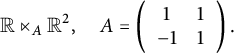 $$\begin{align*}\mathbb{R}\ltimes_A \mathbb{R}^2,\quad A=\left( \begin{array}{cc}1&1\\-1&1\end{array}\right). \end{align*}$$
The family of metrics (described in Theorem 3.8 ) consists of Ricci solitons which are not of constant curvature.
The classification in the case of nonzero divergence is the content of Section 3.3. The unimodular case is covered in Section 3.3, the nonunimodular case in Section 3.3. To keep the introduction succinct, we do only summarize the isomorphism types of the Lie algebras resulting from our classification without listing the detailed solutions, which can be found in Theorem 3.12 and Propositions 3.15 and 3.16.
Theorem 1.4 Any three-dimensional
 $\mathrm {unimodular}$
Lie algebra
$\mathrm {unimodular}$
Lie algebra
 $\mathfrak g$
admits a generalized Einstein structure with
$\mathfrak g$
admits a generalized Einstein structure with
 $\mathrm {nonzero\ divergence}$
as well as a divergence-free solution (see Theorem 3.12
).
$\mathrm {nonzero\ divergence}$
as well as a divergence-free solution (see Theorem 3.12
).
Theorem 1.5 Let
 $(H,g,\delta )$
be a generalized Einstein structure with
$(H,g,\delta )$
be a generalized Einstein structure with
 $\mathrm{nonzero} \mathrm{divergence}$
on a three-dimensional
$\mathrm{nonzero} \mathrm{divergence}$
on a three-dimensional
 $\mathrm {nonunimodular}$
Lie algebra
$\mathrm {nonunimodular}$
Lie algebra
 $\mathfrak g$
. Then either:
$\mathfrak g$
. Then either:
-
(1) The unimodular kernel of
$\mathfrak g$
is nondegenerate (with respect to g) and
$\mathfrak {g} = \mathbb {R}\ltimes _A \mathbb {R}^2$
, where
$$\begin{align*}A=\left( \begin{array}{cc}1&0\\ 0&\lambda\end{array}\right),\mbox{ }\lambda \in (-1,1],\mbox{ and }\, H \neq 0\end{align*}$$
(see Proposition 3.15 for a complete description of
$(H,g,\delta )$
). -
(2) Its unimodular kernel is degenerate,
$H=0$
and
$\mathfrak {g} = \mathbb {R}\ltimes _A \mathbb {R}^2$
, where
$A\in \mathfrak {gl}(2,\mathbb {R})$
is arbitrary with only real eigenvalues and such that
$\mathrm{tr}\, A \neq 0$
(see Proposition 3.16
).


In Proposition 3.17, we indicate for which of the left-invariant generalized Einstein structures the divergence
 $\delta $
coincides with the Riemannian divergence. We find that this is not only the case for all divergence-free solutions on unimodular Lie algebras but also for some of the nonunimodular cases with nonzero divergence. In the latter case, the unimodular kernel can be both degenerate or nondegenerate with respect to the metric g.
$\delta $
coincides with the Riemannian divergence. We find that this is not only the case for all divergence-free solutions on unimodular Lie algebras but also for some of the nonunimodular cases with nonzero divergence. In the latter case, the unimodular kernel can be both degenerate or nondegenerate with respect to the metric g.
For better overview, the results of our classification are summarized in the tables of Section 4.
2 Generalized Einstein metrics on Lie groups
In this section, we develop a general approach for the study of left-invariant generalized Einstein metrics on Lie groups.
2.1 Twisted generalized tangent bundle of a Lie group
Recall that the generalized tangent bundle of a smooth manifold M is the sum
of its tangent and its cotangent bundle and that any closed three-form H on M defines on
 $\mathbb {T}M$
the structure of a Courant algebroid (see, e.g., [Reference García FernándezG, Example 2.5]). We will write
$\mathbb {T}M$
the structure of a Courant algebroid (see, e.g., [Reference García FernándezG, Example 2.5]). We will write
 $\mathbb {T}_pM$
for the fiber at
$\mathbb {T}_pM$
for the fiber at
 $p\in M$
.
$p\in M$
.
Here, we consider only the special case when
 $M=G$
is a Lie group and the Courant algebroid structure is left-invariant.
$M=G$
is a Lie group and the Courant algebroid structure is left-invariant.
Let G be a Lie group with Lie algebra
 $\mathfrak {g}$
and H a closed left-invariant three-form on G. The H-twisted generalized tangent bundle of G is the vector bundle
$\mathfrak {g}$
and H a closed left-invariant three-form on G. The H-twisted generalized tangent bundle of G is the vector bundle
 $\mathbb {T}G\rightarrow G$
endowed with the Courant algebroid structure
$\mathbb {T}G\rightarrow G$
endowed with the Courant algebroid structure
 $(\pi , \langle \cdot ,\cdot \rangle , [\cdot ,\cdot ]_H)$
given by:
$(\pi , \langle \cdot ,\cdot \rangle , [\cdot ,\cdot ]_H)$
given by:
-
(1) The canonical projection
$\pi : \mathbb {T}G \rightarrow TG$
, called the anchor. -
(2) The canonical symmetric bilinear pairing
$\langle \cdot ,\cdot \rangle \in \Gamma (\mathrm {Sym}^2 (\mathbb {T}G)^*)$
, given by
$$\begin{align*}\langle X+\xi , Y+\eta \rangle = \frac12 (\xi (Y) + \eta (Y)),\end{align*}$$
called the scalar product.
-
(3) The (H-twisted) Dorfman bracket
$[\cdot ,\cdot ]_H : \Gamma ( \mathbb {T}G) \times \Gamma ( \mathbb {T}G) \rightarrow \Gamma ( \mathbb {T}G)$
, given by (1)
$$ \begin{align} [ X+\xi , Y + \eta ]_H = \mathcal{L}_X(Y+\eta ) -\iota_Yd\xi + H(X,Y,\cdot ),\end{align} $$
where
$X, Y \in \Gamma (TG)$
,
$\xi , \eta \in \Gamma (T^*G)$
,
$\mathcal {L}$
denotes the Lie derivative and
$\iota $
the interior product.


The above data satisfy the defining axioms of a Courant algebroid:
-
(C1)
$[u,[v,w]_H]_H = [[u,v]_H,w]_H+[v,[u,w]_H]_H$
, -
(C2)
$\pi (u) \langle v,w\rangle = \langle [u,v]_H,w\rangle + \langle v,[u,w]_H\rangle ,$
and -
(C3)
$\pi (u) \langle v,w\rangle = \langle u,[v,w]_H + [w,v]_H\rangle $
,


for all
 $u, v, w\in \Gamma ( \mathbb {T}G)$
. It is well known that the above axioms imply the following useful relations (compare [Reference Cortés and DavidCD, Definition 1] and the references therein), which are obvious from (1).
$u, v, w\in \Gamma ( \mathbb {T}G)$
. It is well known that the above axioms imply the following useful relations (compare [Reference Cortés and DavidCD, Definition 1] and the references therein), which are obvious from (1).
-
• The homomorphism of bundles
$\pi $
is a bracket-homomorphism, that is, where
$$\begin{align*}\pi [u,v]_H = [\pi u,\pi v],\end{align*}$$
$[\pi u,\pi v]= \mathcal {L}_{\pi u}(\pi v)$
denotes the Lie bracket of
$\pi u, \pi v \in \Gamma (TG)$
.
-
• The map
$[u,\cdot ]_H : \Gamma ( \mathbb {T}G) \rightarrow \Gamma ( \mathbb {T}G)$
satisfies the Leibniz rule:
$$\begin{align*}[u,fv ]_H = (\pi u) (f)v + f[u,v]_H,\quad \forall f\in C^{\infty} (M).\end{align*}$$


For notational simplicity, we define
We will identify left-invariant sections of
 $\mathbb {T}G$
(by evaluation at the neutral element
$\mathbb {T}G$
(by evaluation at the neutral element
 $e\in G$
) with elements
$e\in G$
) with elements
and use the same notation to denote them. Correspondingly, the three-form
 $H\in \Gamma ({\bigwedge }^3 T^*G)$
will be identified with an element
$H\in \Gamma ({\bigwedge }^3 T^*G)$
will be identified with an element
 $H\in {\bigwedge }^3 \mathfrak {g}^*$
. With these identifications,
$H\in {\bigwedge }^3 \mathfrak {g}^*$
. With these identifications,
 $\langle \cdot ,\cdot \rangle \in \mathrm {Sym}^2E^*$
and the Dorfman bracket of
$\langle \cdot ,\cdot \rangle \in \mathrm {Sym}^2E^*$
and the Dorfman bracket of
 $X+\xi $
and
$X+\xi $
and
 $Y +\eta \in \mathfrak {g} \oplus \mathfrak {g}^*$
is
$Y +\eta \in \mathfrak {g} \oplus \mathfrak {g}^*$
is
 $$ \begin{align} [ X+\xi , Y + \eta ]_H = [X,Y] -\mathrm{ad}_X^*\eta -\iota_Yd\xi + H(X,Y,\cdot ) \in \mathfrak{g} \oplus \mathfrak{g}^*,\end{align} $$
where
 $[X,Y]$
is the Lie bracket in
$[X,Y]$
is the Lie bracket in
 $\mathfrak {g}$
,
$\mathfrak {g}$
,
 $\mathrm {ad}_X^*\eta = \eta \circ \mathrm {ad}_X$
and d denotes the restriction of the de Rham differential to left-invariant forms, such that
$\mathrm {ad}_X^*\eta = \eta \circ \mathrm {ad}_X$
and d denotes the restriction of the de Rham differential to left-invariant forms, such that
 $-\iota _Yd\xi = \mathrm {ad}_Y^*\xi $
.
$-\iota _Yd\xi = \mathrm {ad}_Y^*\xi $
.
2.2 Generalized metrics on Lie groups
Definition 2.1 A generalized pseudo-Riemannian metric on a manifold M is a section
 $\mathcal G \in \Gamma (\mathrm {Sym}^2(\mathbb {T}M)^*)$
such that the endomorphism
$\mathcal G \in \Gamma (\mathrm {Sym}^2(\mathbb {T}M)^*)$
such that the endomorphism
 $\mathcal {G}^{\mathrm {end}} \in \Gamma (\mathrm {End}\, \mathbb {T}M)$
defined by
$\mathcal {G}^{\mathrm {end}} \in \Gamma (\mathrm {End}\, \mathbb {T}M)$
defined by
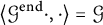 $$ \begin{align} \langle \mathcal{G}^{\mathrm{end}} \cdot ,\cdot \rangle = \mathcal{G}\end{align} $$
is an involution and
 $\mathcal G|_{\mathrm {Sym}^2(T^*M)}$
is nondegenerate. The pair
$\mathcal G|_{\mathrm {Sym}^2(T^*M)}$
is nondegenerate. The pair
 $(M,\mathcal G)$
is called a generalized pseudo-Riemannian manifold. The prefix pseudo will be omitted when
$(M,\mathcal G)$
is called a generalized pseudo-Riemannian manifold. The prefix pseudo will be omitted when
 $\mathcal G$
is positive definite.
$\mathcal G$
is positive definite.
Note that for a generalized metric, equation (5) is equivalent to
 $\mathcal {G}^{\mathrm {end}}=\mathcal {G}^{-1}\circ \langle \cdot ,\cdot \rangle $
, using the identification
$\mathcal {G}^{\mathrm {end}}=\mathcal {G}^{-1}\circ \langle \cdot ,\cdot \rangle $
, using the identification
 $(\mathbb {T}M)^*\otimes (\mathbb {T}M)^* = \mathrm {Hom}(\mathbb {T}M,(\mathbb {T}M)^*)$
given by evaluation in the first argument. We do also remark that the nondegeneracy of
$(\mathbb {T}M)^*\otimes (\mathbb {T}M)^* = \mathrm {Hom}(\mathbb {T}M,(\mathbb {T}M)^*)$
given by evaluation in the first argument. We do also remark that the nondegeneracy of
 $\mathcal G|_{\mathrm {Sym}^2(T^*M)}$
is automatic if
$\mathcal G|_{\mathrm {Sym}^2(T^*M)}$
is automatic if
 $\mathcal G$
is positive or negative definite.
$\mathcal G$
is positive or negative definite.
A left-invariant generalized metric on a Lie group G is identified (by evaluation at the neutral element
 $e\in G$
) with a generalized metric on
$e\in G$
) with a generalized metric on
 $\mathfrak {g} =\mathrm {Lie}\, G$
as defined in the following definition.
$\mathfrak {g} =\mathrm {Lie}\, G$
as defined in the following definition.
Definition 2.2 Let H be a left-invariant closed three-form on a Lie group G, which we identify (by evaluation at
 $e\in G$
) with an element
$e\in G$
) with an element
 $H\in \bigwedge ^3\mathfrak {g}^*$
. A generalized (pseudo-Riemannian) metric on its Lie algebra
$H\in \bigwedge ^3\mathfrak {g}^*$
. A generalized (pseudo-Riemannian) metric on its Lie algebra
 $\mathfrak {g} =\mathrm {Lie}\, G$
is a symmetric bilinear form
$\mathfrak {g} =\mathrm {Lie}\, G$
is a symmetric bilinear form
 $\mathcal G \in \mathrm {Sym}^2E^*$
(cf. (3)) such that
$\mathcal G \in \mathrm {Sym}^2E^*$
(cf. (3)) such that
 $\mathcal {G}^{\mathrm {end}}=\mathcal {G}^{-1}\circ \langle \cdot ,\cdot \rangle $
is an involution and
$\mathcal {G}^{\mathrm {end}}=\mathcal {G}^{-1}\circ \langle \cdot ,\cdot \rangle $
is an involution and
 $\mathcal G|_{\mathrm {Sym}^2\mathfrak g^*}$
is nondegenerate. The corresponding triple
$\mathcal G|_{\mathrm {Sym}^2\mathfrak g^*}$
is nondegenerate. The corresponding triple
 $(G,H,\mathcal G)$
will be called a pseudo-Riemannian generalized Lie group and
$(G,H,\mathcal G)$
will be called a pseudo-Riemannian generalized Lie group and
 $(\mathfrak g,H,\mathcal G)$
a pseudo-Riemannian generalized Lie algebra. The prefix pseudo will be omitted when
$(\mathfrak g,H,\mathcal G)$
a pseudo-Riemannian generalized Lie algebra. The prefix pseudo will be omitted when
 $\mathcal G$
is positive definite.
$\mathcal G$
is positive definite.
Two pseudo-Riemannian generalized Lie groups
 $(G,H,\mathcal G)$
and
$(G,H,\mathcal G)$
and
 $(G',H',\mathcal G')$
are called isomorphic if there exists an isomorphism of Lie groups
$(G',H',\mathcal G')$
are called isomorphic if there exists an isomorphism of Lie groups
 $\varphi : G \rightarrow G'$
and an isomorphism of bundles
$\varphi : G \rightarrow G'$
and an isomorphism of bundles
 $\Phi : \mathbb {T}G \rightarrow \mathbb {T}G '$
covering
$\Phi : \mathbb {T}G \rightarrow \mathbb {T}G '$
covering
 $\varphi $
such that
$\varphi $
such that
 $\Phi $
maps the Courant algebroid structure
$\Phi $
maps the Courant algebroid structure
 $(\pi , \langle \cdot , \cdot \rangle , [\cdot ,\cdot ]_H)$
on G determined by H to the Courant algebroid structure on
$(\pi , \langle \cdot , \cdot \rangle , [\cdot ,\cdot ]_H)$
on G determined by H to the Courant algebroid structure on
 $G'$
determined by
$G'$
determined by
 $H'$
and the generalized metric
$H'$
and the generalized metric
 $\mathcal {G}$
to the generalized metric
$\mathcal {G}$
to the generalized metric
 $\mathcal {G}'$
. The map
$\mathcal {G}'$
. The map
 $\Phi $
is called an isomorphism of pseudo-Riemannian generalized Lie groups.
$\Phi $
is called an isomorphism of pseudo-Riemannian generalized Lie groups.
Similarly, two pseudo-Riemannian generalized Lie algebras
 $(\mathfrak g,H,\mathcal G)$
and
$(\mathfrak g,H,\mathcal G)$
and
 $(\mathfrak g',H',\mathcal G')$
are called isomorphic if there exists an isomorphism of Lie algebras
$(\mathfrak g',H',\mathcal G')$
are called isomorphic if there exists an isomorphism of Lie algebras
 $\varphi : \mathfrak g \rightarrow \mathfrak g'$
and an isomorphism of vector spaces
$\varphi : \mathfrak g \rightarrow \mathfrak g'$
and an isomorphism of vector spaces
 $\phi : E(\mathfrak g )\rightarrow E(\mathfrak {g}')$
covering
$\phi : E(\mathfrak g )\rightarrow E(\mathfrak {g}')$
covering
 $\varphi $
which maps the data
$\varphi $
which maps the data
 $(\langle \cdot , \cdot \rangle , [\cdot ,\cdot ]_H, \mathcal G)$
on
$(\langle \cdot , \cdot \rangle , [\cdot ,\cdot ]_H, \mathcal G)$
on
 $\mathfrak {g}$
(cf. (4)) to the data
$\mathfrak {g}$
(cf. (4)) to the data
 $(\langle \cdot , \cdot \rangle ' , [\cdot ,\cdot ]_{H'}, \mathcal G')$
on
$(\langle \cdot , \cdot \rangle ' , [\cdot ,\cdot ]_{H'}, \mathcal G')$
on
 $\mathfrak {g}'$
. Here,
$\mathfrak {g}'$
. Here,
 $\langle \cdot ,\cdot \rangle '$
denotes the canonical symmetric pairing on
$\langle \cdot ,\cdot \rangle '$
denotes the canonical symmetric pairing on
 $E(\mathfrak g')$
induced by the duality between
$E(\mathfrak g')$
induced by the duality between
 $\mathfrak g'$
and
$\mathfrak g'$
and
 $(\mathfrak g')^*$
. The map
$(\mathfrak g')^*$
. The map
 $\phi $
is called an isomorphism of pseudo-Riemannian generalized Lie algebras.
$\phi $
is called an isomorphism of pseudo-Riemannian generalized Lie algebras.
Example 2.3 Let g be a left-invariant pseudo-Riemannian metric on G. We denote the corresponding bilinear form on the Lie algebra
 $\mathfrak g$
by the same symbol:
$\mathfrak g$
by the same symbol:
 $g\in \mathrm {Sym}^2\mathfrak g^*$
. It extends to a generalized metric
$g\in \mathrm {Sym}^2\mathfrak g^*$
. It extends to a generalized metric
 $\mathcal {G}_g\in \mathrm {Sym}^2E^*$
such that
$\mathcal {G}_g\in \mathrm {Sym}^2E^*$
such that
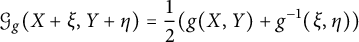 $$\begin{align*}\mathcal{G}_g(X+\xi , Y+\eta ) = \frac12 (g(X,Y) + g^{-1}(\xi ,\eta))\end{align*}$$
for all
 $X+\xi , Y+\eta \in E$
. The corresponding endomorphism
$X+\xi , Y+\eta \in E$
. The corresponding endomorphism
 $\mathcal {G}^{\mathrm {end}}$
is
$\mathcal {G}^{\mathrm {end}}$
is
 $$\begin{align*}\mathcal{G}^{\mathrm{end}}=g \oplus g^{-1} : E=\mathfrak g \oplus \mathfrak g^* \rightarrow E^* = \mathfrak g^* \oplus \mathfrak g.\end{align*}$$
Proposition 2.4 Let
 $(G,H,\mathcal G)$
be a pseudo-Riemannian generalized Lie group. Then there exist a left-invariant pseudo-Riemannian metric g on G and a closed left-invariant three-form
$(G,H,\mathcal G)$
be a pseudo-Riemannian generalized Lie group. Then there exist a left-invariant pseudo-Riemannian metric g on G and a closed left-invariant three-form
 $H'\in [H]\in H^3(\mathfrak {g})$
such that
$H'\in [H]\in H^3(\mathfrak {g})$
such that
 $(G,H,\mathcal G)$
is isomorphic to
$(G,H,\mathcal G)$
is isomorphic to
 $(G,H',\mathcal {G}_g)$
, by an isomorphism
$(G,H',\mathcal {G}_g)$
, by an isomorphism
 $\Phi $
covering the identity map of G.
$\Phi $
covering the identity map of G.
Proof The decomposition
 $E = \mathfrak g \oplus \mathfrak g^*$
gives rise to the following block decomposition
$E = \mathfrak g \oplus \mathfrak g^*$
gives rise to the following block decomposition
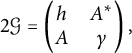 $$\begin{align*}2 \mathcal G = \left( \begin{array}{@{}cc@{}}h&A^*\\ A&\gamma \end{array}\right) ,\end{align*}$$
where
 $h\in \mathrm {Sym}^2\mathfrak g$
,
$h\in \mathrm {Sym}^2\mathfrak g$
,
 $A\in \mathrm {End} (\mathfrak g)$
and
$A\in \mathrm {End} (\mathfrak g)$
and
 $\gamma \in \mathrm {Sym}^2\mathfrak g^*$
is nondegenerate, as follows from the symmetry of
$\gamma \in \mathrm {Sym}^2\mathfrak g^*$
is nondegenerate, as follows from the symmetry of
 $\mathcal G$
and the nondegeneracy of
$\mathcal G$
and the nondegeneracy of
 $\mathcal G|_{\mathrm {Sym}^2 \mathfrak {g}^*}$
. In terms of
$\mathcal G|_{\mathrm {Sym}^2 \mathfrak {g}^*}$
. In terms of
![]() , we can write the necessary and sufficient conditions for
, we can write the necessary and sufficient conditions for
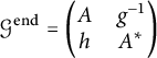 $$ \begin{align} \mathcal{G}^{\mathrm{end}} = \left( \begin{array}{@{}cc@{}}A&g^{-1}\\ h& A^* \end{array}\right)\end{align} $$
to be an involution as
 $$\begin{align*}A^2 + g^{-1}h= \mathbf{1},\quad gA = -A^*g,\quad h A =- A^*h,\end{align*}$$
where the last two equations mean that A is skew-symmetric for g and h. In particular, we can write
 $A = -g^{-1}\beta $
for some
$A = -g^{-1}\beta $
for some
 $\beta \in \bigwedge ^2\mathfrak g^*$
. Solving the first equation for h, we obtain
$\beta \in \bigwedge ^2\mathfrak g^*$
. Solving the first equation for h, we obtain
 $$\begin{align*}h = g -gA^2 = g +\beta A = g -\beta g^{-1} \beta .\end{align*}$$
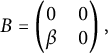
This implies that
 $\mathcal {G}^{\mathrm {end}} = \exp (B) (\mathcal {G}_g)^{\mathrm {end}} \exp (-B)$
, where
$\mathcal {G}^{\mathrm {end}} = \exp (B) (\mathcal {G}_g)^{\mathrm {end}} \exp (-B)$
, where
 $$\begin{align*}B = \left( \begin{array}{@{}cc@{}}0&0\\ \beta & 0 \end{array}\right),\end{align*}$$
or equivalently,
 $\mathcal {G} = \exp (-B)^*\mathcal {G}_g$
. Now it suffices to check that the map
$\mathcal {G} = \exp (-B)^*\mathcal {G}_g$
. Now it suffices to check that the map
 $$\begin{align*}\phi = \exp (-B) : E \rightarrow E,\quad X+\xi \mapsto X+\xi - \beta X,\end{align*}$$
defines an isomorphism of pseudo-Riemannian generalized Lie algebras from
 $(\mathfrak g, H,\mathcal G)$
to
$(\mathfrak g, H,\mathcal G)$
to
 $(\mathfrak g, H',\mathcal G_g)$
covering the identity map of
$(\mathfrak g, H',\mathcal G_g)$
covering the identity map of
 $\mathfrak g$
, where
$\mathfrak g$
, where
 $H'=H+d\beta $
. The corresponding isomorphism
$H'=H+d\beta $
. The corresponding isomorphism
 $\Phi $
of pseudo-Riemannian generalized Lie groups is also given by
$\Phi $
of pseudo-Riemannian generalized Lie groups is also given by
 $\exp (-B)$
, now considered as an endomorphism of
$\exp (-B)$
, now considered as an endomorphism of
 $\mathbb {T}G$
.
$\mathbb {T}G$
.
Remark 2.5 Clearly, a decomposition of the form (6) holds for any generalized pseudo-Riemannian metric
 $\mathcal {G}$
on a manifold M. This shows that
$\mathcal {G}$
on a manifold M. This shows that
 $\operatorname {\mathrm{tr}} \mathcal {G}^{\mathrm {end}}=0$
, since A is skew-symmetric with respect to g.
$\operatorname {\mathrm{tr}} \mathcal {G}^{\mathrm {end}}=0$
, since A is skew-symmetric with respect to g.
2.3 Space of left-invariant Levi-Civita generalized connections
Let H be a closed three-form on a smooth manifold M and consider
 $\mathbb {T}M$
with the Courant algebroid structure defined by H.
$\mathbb {T}M$
with the Courant algebroid structure defined by H.
Definition 2.6 A generalized connection on M is a linear map
 $$\begin{align*}D : \Gamma (\mathbb{T}M) \rightarrow \Gamma ((\mathbb{T}M)^*\otimes \mathbb{T}M),\quad v \mapsto Dv = (u\mapsto D_uv),\end{align*}$$
such that:
-
(1)
$D_u(fv) = u(f) v + fD_uv$
(anchored Leibniz rule), recall (2), and -
(2)
$u\langle v,w\rangle = \langle D_uv,w\rangle + \langle v,D_uw\rangle $


for all
 $u, v, w\in \Gamma (\mathbb {T}M)$
. The torsion of a generalized connection D (with respect to the Dorfman bracket
$u, v, w\in \Gamma (\mathbb {T}M)$
. The torsion of a generalized connection D (with respect to the Dorfman bracket
 $[\cdot ,\cdot ]_H$
) is the section
$[\cdot ,\cdot ]_H$
) is the section
 $T\in \Gamma (\bigwedge ^2 (\mathbb {T}M)^*\otimes \mathbb {T}M)$
defined by
$T\in \Gamma (\bigwedge ^2 (\mathbb {T}M)^*\otimes \mathbb {T}M)$
defined by
where
 $(Du)^*$
is the adjoint of
$(Du)^*$
is the adjoint of
 $Du$
with respect to the scalar product (cf. [Reference García FernándezG]). The generalized connection D is called torsion-free if
$Du$
with respect to the scalar product (cf. [Reference García FernándezG]). The generalized connection D is called torsion-free if
 $T=0$
.
$T=0$
.
Given a generalized pseudo-Riemannian metric
 $\mathcal G$
on M, we say that a generalized connection D is metric if
$\mathcal G$
on M, we say that a generalized connection D is metric if
 $D\mathcal G=0$
, where
$D\mathcal G=0$
, where
 $D_u : \Gamma (\mathbb {T}M)\rightarrow \Gamma (\mathbb {T}M)$
is extended to space of sections of the tensor algebra over
$D_u : \Gamma (\mathbb {T}M)\rightarrow \Gamma (\mathbb {T}M)$
is extended to space of sections of the tensor algebra over
 $\mathbb {T}M$
as a tensor derivation for all
$\mathbb {T}M$
as a tensor derivation for all
 $u\in \Gamma (\mathbb {T}M)$
. More explicitly, the latter condition is
$u\in \Gamma (\mathbb {T}M)$
. More explicitly, the latter condition is
 $$\begin{align*}u\mathcal{G}(v,w) = \mathcal{G}(D_uv,w) + \mathcal{G}(v,D_uw),\quad \forall u,v,w\in \Gamma (\mathbb{T}M).\end{align*}$$
This condition is satisfied if and only if D preserves the eigenbundles of
 $\mathcal {G}^{\mathrm {end}}$
.
$\mathcal {G}^{\mathrm {end}}$
.
Any metric and torsion-free generalized connection on a generalized pseudo-Riemannian manifold
 $(M,\mathcal G)$
(endowed with the three-form H) is called a Levi-Civita generalized connection.
$(M,\mathcal G)$
(endowed with the three-form H) is called a Levi-Civita generalized connection.
It is known [Reference García FernándezG] that the torsion of a generalized connection is totally skew, that is,
 $T\in \Gamma (\bigwedge ^2 (\mathbb {T}M)^*\otimes \mathbb {T}M)$
defines a section of
$T\in \Gamma (\bigwedge ^2 (\mathbb {T}M)^*\otimes \mathbb {T}M)$
defines a section of
 $\bigwedge ^3 (\mathbb {T}M)^*$
upon identification
$\bigwedge ^3 (\mathbb {T}M)^*$
upon identification
 $\mathbb {T}M\cong (\mathbb {T}M)^*$
using the scalar product.
$\mathbb {T}M\cong (\mathbb {T}M)^*$
using the scalar product.
Given a reduction of the structure group
 $\mathrm {O}(n,n)$
of
$\mathrm {O}(n,n)$
of
 $\mathbb {T}M$
,
$\mathbb {T}M$
,
 $n=\dim M$
, to a subgroup
$n=\dim M$
, to a subgroup
 $L= \mathrm {O}(n,n)_S\subset \mathrm {O}(n,n)$
defined by a tensor
$L= \mathrm {O}(n,n)_S\subset \mathrm {O}(n,n)$
defined by a tensor
 $S\in \bigoplus _{k=0}^{\infty } \bigotimes ^k \left (\mathbb {R}^n\oplus (\mathbb {R}^n)^*\right )$
, we consider the tensor field
$S\in \bigoplus _{k=0}^{\infty } \bigotimes ^k \left (\mathbb {R}^n\oplus (\mathbb {R}^n)^*\right )$
, we consider the tensor field
 $\mathcal S$
which in any frame of the reduction has the same coefficients as S in the standard basis of
$\mathcal S$
which in any frame of the reduction has the same coefficients as S in the standard basis of
 $\mathbb {R}^n\oplus (\mathbb {R}^n)^*$
. A generalized connection D is called compatible with the L-reduction if
$\mathbb {R}^n\oplus (\mathbb {R}^n)^*$
. A generalized connection D is called compatible with the L-reduction if
 $D\mathcal S =0$
. It was shown in [Reference Cortés and DavidCD] that a torsion-free generalized connection (on a Courant algebroid) compatible with an L-reduction exists if and only if its intrinsic torsion (defined in [Reference Cortés and DavidCD, Definition 15]) vanishes. In that case, it was also shown there that the space of compatible torsion-free generalized connections is an affine space modeled on the space of sections of the generalized first prolongation
$D\mathcal S =0$
. It was shown in [Reference Cortés and DavidCD] that a torsion-free generalized connection (on a Courant algebroid) compatible with an L-reduction exists if and only if its intrinsic torsion (defined in [Reference Cortés and DavidCD, Definition 15]) vanishes. In that case, it was also shown there that the space of compatible torsion-free generalized connections is an affine space modeled on the space of sections of the generalized first prolongation
 $(\mathfrak {so}(\mathbb {T}M)_{\mathcal {S}})^{\langle 1\rangle }$
(defined in [Reference Cortés and DavidCD, Definition 16]) of
$(\mathfrak {so}(\mathbb {T}M)_{\mathcal {S}})^{\langle 1\rangle }$
(defined in [Reference Cortés and DavidCD, Definition 16]) of
 $\mathfrak {so}(\mathbb {T}M)_{\mathcal {S}}$
. Note that the fiber of the bundle
$\mathfrak {so}(\mathbb {T}M)_{\mathcal {S}}$
. Note that the fiber of the bundle
 $\mathfrak {so}(\mathbb {T}M)_{\mathcal {S}}$
at a point
$\mathfrak {so}(\mathbb {T}M)_{\mathcal {S}}$
at a point
 $p\in M$
is
$p\in M$
is
 $\mathfrak {so}(\mathbb {T}_pM)_{\mathcal {S}_p}\cong \mathfrak {so}(n,n)_{S}=\mathfrak {l} = \mathrm {Lie}\, L$
, so that
$\mathfrak {so}(\mathbb {T}_pM)_{\mathcal {S}_p}\cong \mathfrak {so}(n,n)_{S}=\mathfrak {l} = \mathrm {Lie}\, L$
, so that
 $(\mathfrak {so}(\mathbb {T}M)_{\mathcal {S}})^{\langle 1\rangle }|_p\cong \mathfrak {l}^{\langle 1\rangle }$
.
$(\mathfrak {so}(\mathbb {T}M)_{\mathcal {S}})^{\langle 1\rangle }|_p\cong \mathfrak {l}^{\langle 1\rangle }$
.
As a special case, we can apply the above theory to the case when
 $\mathcal S = \mathcal G$
is a generalized pseudo-Riemannian metric. The existence of a Levi-Civita generalized connection shown in [Reference García FernándezG, Proposition 3.3] implies the following.
$\mathcal S = \mathcal G$
is a generalized pseudo-Riemannian metric. The existence of a Levi-Civita generalized connection shown in [Reference García FernándezG, Proposition 3.3] implies the following.
Proposition 2.7 Let
 $(M,\mathcal {G})$
be a generalized pseudo-Riemannian manifold and H a closed three-form on M. Then the space of Levi-Civita generalized connections (with respect to the H-twisted Dorfman bracket) is an affine space modeled on
$(M,\mathcal {G})$
be a generalized pseudo-Riemannian manifold and H a closed three-form on M. Then the space of Levi-Civita generalized connections (with respect to the H-twisted Dorfman bracket) is an affine space modeled on
 $(\mathfrak {so}(\mathbb {T}M)_{\mathcal {G}})^{\langle 1\rangle }$
.
$(\mathfrak {so}(\mathbb {T}M)_{\mathcal {G}})^{\langle 1\rangle }$
.
A generalized connection D on a Lie group G is called left-invariant if
 $D_uv\in \Gamma (\mathbb {T}G)$
is left-invariant for all left-invariant sections
$D_uv\in \Gamma (\mathbb {T}G)$
is left-invariant for all left-invariant sections
 $u,v\in \Gamma (\mathbb {T}G)$
. A left-invariant generalized connection on G can be identified with an element
$u,v\in \Gamma (\mathbb {T}G)$
. A left-invariant generalized connection on G can be identified with an element
 $D\in E^*\otimes \mathfrak {so}(E)$
, where we recall that
$D\in E^*\otimes \mathfrak {so}(E)$
, where we recall that
 $E=\mathfrak {g} \oplus \mathfrak {g}^*$
. Its torsion T is identified with an element
$E=\mathfrak {g} \oplus \mathfrak {g}^*$
. Its torsion T is identified with an element
 $T\in (\bigwedge ^2E^*\otimes E)\cap (E^*\otimes \mathfrak {so}(E))\cong \bigwedge ^3 E^*$
. We denote by
$T\in (\bigwedge ^2E^*\otimes E)\cap (E^*\otimes \mathfrak {so}(E))\cong \bigwedge ^3 E^*$
. We denote by
 $E_+$
and
$E_+$
and
 $E_-$
the eigenspaces of
$E_-$
the eigenspaces of
 $\mathcal {G}^{\mathrm {end}}\in \mathrm {End}(E)$
for the eigenvalues
$\mathcal {G}^{\mathrm {end}}\in \mathrm {End}(E)$
for the eigenvalues
 $\pm 1$
, respectively. Note that
$\pm 1$
, respectively. Note that
 $\dim E_+ =\dim E_- =\dim G =:n$
by Remark 2.5.
$\dim E_+ =\dim E_- =\dim G =:n$
by Remark 2.5.
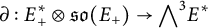
Proposition 2.8 Let
 $(G,H,\mathcal G)$
be a pseudo-Riemannian generalized Lie group. Then the space of left-invariant Levi-Civita generalized connections on G is an affine space modeled on
$(G,H,\mathcal G)$
be a pseudo-Riemannian generalized Lie group. Then the space of left-invariant Levi-Civita generalized connections on G is an affine space modeled on
 $\mathfrak {so}(E)^{\langle 1\rangle } = \Sigma _+ \oplus \Sigma _-$
, where
$\mathfrak {so}(E)^{\langle 1\rangle } = \Sigma _+ \oplus \Sigma _-$
, where
 $\Sigma _+ \subset E_+^*\otimes \mathfrak {so}(E_+)$
is the kernel of the map
$\Sigma _+ \subset E_+^*\otimes \mathfrak {so}(E_+)$
is the kernel of the map
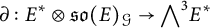
 $$\begin{align*}\partial : E_+^*\otimes \mathfrak{so}(E_+) \rightarrow {\bigwedge}^3 E^*\end{align*}$$
defined by
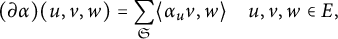 $$ \begin{align} (\partial \alpha ) (u,v,w) = \sum_{\mathfrak{S}} \langle \alpha_uv,w\rangle \quad u,v,w\in E, \end{align} $$
and similarly for
 $\Sigma _-\subset E_-^*\otimes \mathfrak {so}(E_-)$
. Here,
$\Sigma _-\subset E_-^*\otimes \mathfrak {so}(E_-)$
. Here,
 $\mathfrak {S}$
indicates the sum over the cyclic permutations and
$\mathfrak {S}$
indicates the sum over the cyclic permutations and
 $\alpha _u\in \mathfrak {so}(E_+)$
stands for evaluation of
$\alpha _u\in \mathfrak {so}(E_+)$
stands for evaluation of
 $\alpha \in E_+^*\otimes \mathfrak {so}(E_+) = \mathrm {Hom}(E_+,\mathfrak {so}(E_+))$
at u.
$\alpha \in E_+^*\otimes \mathfrak {so}(E_+) = \mathrm {Hom}(E_+,\mathfrak {so}(E_+))$
at u.
Moreover,
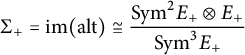 $$\begin{align*}\Sigma_+ = \mathrm{im} (\mathrm{alt}) \cong \frac{\mathrm{Sym}^2 E_+\otimes E_+}{\mathrm{Sym}^3E_+}\end{align*}$$
is the image of the map
 $$\begin{align*}\mathrm{alt} : \mathrm{Sym}^2 E_+^* \otimes E_+^*\rightarrow E_+^*\otimes \mathfrak{so}(E_+)\end{align*}$$
defined by
 $$\begin{align*}\langle \mathrm{alt}(\sigma)_uv,w\rangle = \sigma (u,v,w) -\sigma (u,w,v)\end{align*}$$
and similarly for
 $\Sigma _-$
.
$\Sigma _-$
.
Proof The first part of the proposition follows easily from the existence of a left-invariant Levi-Civita generalized connection (to be shown at the end of the proof), Proposition 2.7 and the definition of the generalized first prolongation [Reference Cortés and DavidCD] as the kernel of the natural map
 $$\begin{align*}\partial : E^*\otimes \mathfrak{so}(E)_{\mathcal{G}} \rightarrow {\bigwedge}^3 E^*\end{align*}$$
given by the formula (7). To compute the kernel, we can first observe that
 $\mathfrak {so}(E)_{\mathcal {G}} = \mathfrak {so}(E_+) \oplus \mathfrak {so}(E_-)\cong \bigwedge ^2 E_+^* \oplus \bigwedge ^2 E_-^*$
. Since
$\mathfrak {so}(E)_{\mathcal {G}} = \mathfrak {so}(E_+) \oplus \mathfrak {so}(E_-)\cong \bigwedge ^2 E_+^* \oplus \bigwedge ^2 E_-^*$
. Since
 $\partial $
maps
$\partial $
maps
 $E_{\epsilon _1}^*\otimes \mathfrak {so}(E_{\epsilon _2})$
to
$E_{\epsilon _1}^*\otimes \mathfrak {so}(E_{\epsilon _2})$
to
 $E_{\epsilon _1}^*\wedge E_{\epsilon _2}^*\wedge E_{\epsilon _2}^* \subset \bigwedge ^3 E^*$
,
$E_{\epsilon _1}^*\wedge E_{\epsilon _2}^*\wedge E_{\epsilon _2}^* \subset \bigwedge ^3 E^*$
,
 $\epsilon _1, \epsilon _2 \in \{ -1, 1\}$
, it suffices to consider the kernels of these four restrictions. On tensors of mixed type
$\epsilon _1, \epsilon _2 \in \{ -1, 1\}$
, it suffices to consider the kernels of these four restrictions. On tensors of mixed type
 $\partial $
is injective, such that
$\partial $
is injective, such that
 $\ker \partial = \Sigma _+ \oplus \Sigma _-$
. The last part of the corollary follows from the exact sequence
$\ker \partial = \Sigma _+ \oplus \Sigma _-$
. The last part of the corollary follows from the exact sequence
 $$ \begin{align} 0\rightarrow \mathrm{Sym}^3V\rightarrow \mathrm{Sym}^2V\otimes V \stackrel{\mathrm{alt}_V}{\longrightarrow} V \otimes {\bigwedge}^2 V \stackrel{\partial_V}{\longrightarrow} {\bigwedge}^3V\rightarrow 0\end{align} $$
that holds for any finite-dimensional vector space V and was used in [Reference García FernándezG]. Here,
 $\mathrm {alt}_V$
is given by
$\mathrm {alt}_V$
is given by
 $$\begin{align*}(u\otimes v + v\otimes u)\otimes w \mapsto u\otimes v\wedge w + v\otimes w \wedge u\end{align*}$$
and
 $\partial _V$
by
$\partial _V$
by
 $$\begin{align*}u\otimes v\wedge w \mapsto u\wedge v\wedge w.\end{align*}$$
We apply the sequence to
 $V=E_+$
(and similarly to
$V=E_+$
(and similarly to
 $V=E_-$
) using the metric identifications
$V=E_-$
) using the metric identifications
 $E_+ \cong E_+^*$
and
$E_+ \cong E_+^*$
and
 $\mathfrak {so}(E_+) \cong \bigwedge ^2E_+^*\cong \bigwedge ^2E_+$
, which allow to identify the natural maps
$\mathfrak {so}(E_+) \cong \bigwedge ^2E_+^*\cong \bigwedge ^2E_+$
, which allow to identify the natural maps
 $\mathrm {alt}_V$
and
$\mathrm {alt}_V$
and
 $\partial _V$
with
$\partial _V$
with
 $\mathrm {alt}: \mathrm {Sym}^2E_+^*\otimes E_+^* \rightarrow E_+^* \otimes \mathfrak {so}(E_+ )$
and
$\mathrm {alt}: \mathrm {Sym}^2E_+^*\otimes E_+^* \rightarrow E_+^* \otimes \mathfrak {so}(E_+ )$
and
 $\partial : E_+^* \otimes \mathfrak {so}(E_+ ) \rightarrow \bigwedge ^3 E_+^*$
, respectively.
$\partial : E_+^* \otimes \mathfrak {so}(E_+ ) \rightarrow \bigwedge ^3 E_+^*$
, respectively.
Now it suffices to show that there exists a left-invariant Levi-Civita generalized connection. We consider the tensor
 $\mathcal {B} \in \bigotimes ^3 E^*$
defined by
$\mathcal {B} \in \bigotimes ^3 E^*$
defined by
 $$ \begin{align} \mathcal{B}(u,v,w) = \langle [u,v]_H,w\rangle,\quad u,v,w\in E. \end{align} $$
Lemma 2.9
 $\mathcal {B}$
is totally skew.
$\mathcal {B}$
is totally skew.
Proof The skew-symmetry in
 $(u,v)$
follows from axiom
$(u,v)$
follows from axiom
 $C3$
in Section 2.1:
$C3$
in Section 2.1:
 $$\begin{align*}\mathcal{B}(u,v,w)+\mathcal{B}(v,u,w)= \langle w, [u,v]_H+[v,u]_H\rangle = w\langle u,v\rangle =0,\end{align*}$$
since
 $\langle u,v\rangle $
is a constant function. Using axiom C2, we obtain
$\langle u,v\rangle $
is a constant function. Using axiom C2, we obtain
 $$\begin{align*}\mathcal{B}(u,v,w) = \langle [u,v]_H,w\rangle = u\langle v,w\rangle -\langle v,[u,w]_H\rangle = -\mathcal{B}(u,w,v).\end{align*}$$
Now it suffices to observe that skew-symmetry in
 $(u,v)$
and
$(u,v)$
and
 $(v,w)$
implies total skew-symmetry.
$(v,w)$
implies total skew-symmetry.
Next, we define
As an element of
 $E^*\otimes \bigwedge ^2 E^*\cong E^*\otimes \mathfrak {so}(E)$
, it defines a left-invariant generalized connection. It is metric, since it takes values in the subalgebra
$E^*\otimes \bigwedge ^2 E^*\cong E^*\otimes \mathfrak {so}(E)$
, it defines a left-invariant generalized connection. It is metric, since it takes values in the subalgebra
 $\mathfrak {so}(E_+)\oplus \mathfrak {so}(E_-) \subset \mathfrak {so}(E)$
. Since
$\mathfrak {so}(E_+)\oplus \mathfrak {so}(E_-) \subset \mathfrak {so}(E)$
. Since
 $\partial \mathcal {B}|_{\bigwedge ^3E_{\pm }} = 3 \mathcal {B}|_{\bigwedge ^3E_{\pm }}$
and
$\partial \mathcal {B}|_{\bigwedge ^3E_{\pm }} = 3 \mathcal {B}|_{\bigwedge ^3E_{\pm }}$
and
 $\partial \mathcal {B}|_{E_{\mp }\otimes \bigwedge ^2 E_{\pm }}= \mathcal {B}|_{E_{\mp }\wedge E_{\pm }\wedge E_{\pm }}$
, the torsion
$\partial \mathcal {B}|_{E_{\mp }\otimes \bigwedge ^2 E_{\pm }}= \mathcal {B}|_{E_{\mp }\wedge E_{\pm }\wedge E_{\pm }}$
, the torsion
 $T^{D^0}= \partial D^0 -\mathcal {B}$
of
$T^{D^0}= \partial D^0 -\mathcal {B}$
of
 $D^0$
is given by
$D^0$
is given by
 $$\begin{align*}T^{D^0}= \left( \mathcal{B}|_{\bigwedge^3E_+} \oplus \mathcal{B}|_{\bigwedge^3E_-}\oplus \partial \mathcal{B}|_{E_+\otimes \bigwedge^2 E_-} \oplus \partial \mathcal{B}|_{E_-\otimes \bigwedge^2 E_+}\right) -\mathcal{B} = \mathcal{B} -\mathcal{B}=0.\end{align*}$$
Remark 2.10 Note that due to Lemma 2.9 and the Jacobi identity (axiom C1), the tensor
 $\mathcal {B}$
together with the scalar product
$\mathcal {B}$
together with the scalar product
 $\langle \cdot , \cdot \rangle $
defines on
$\langle \cdot , \cdot \rangle $
defines on
 $E(\mathfrak {g})$
the structure of a quadratic Lie algebra. Such algebras are examples of Courant algebroids with trivial anchor. Generalized metrics, generalized connections, and curvature on quadratic Lie algebras have been studied in [Reference Álvarez-Cónsul, De Arriba de La Hera and Garcia-FernandezADG]. Their formulas are consistent with ours.
$E(\mathfrak {g})$
the structure of a quadratic Lie algebra. Such algebras are examples of Courant algebroids with trivial anchor. Generalized metrics, generalized connections, and curvature on quadratic Lie algebras have been studied in [Reference Álvarez-Cónsul, De Arriba de La Hera and Garcia-FernandezADG]. Their formulas are consistent with ours.
2.4 Levi-Civita generalized connections with prescribed divergence
In this subsection, we show that every left-invariant divergence operator on the generalized tangent bundle of a generalized pseudo-Riemannian Lie group admits a compatible left-invariant Levi-Civita generalized connection. We then give an explicit construction of such a generalized connection in the case when
 $\mathcal G$
is associated with a left-invariant pseudo-Riemannian metric as in Example 2.3. In view of Proposition 2.4, there is no loss in generality by considering this special case.
$\mathcal G$
is associated with a left-invariant pseudo-Riemannian metric as in Example 2.3. In view of Proposition 2.4, there is no loss in generality by considering this special case.
Definition 2.11 A divergence operator on
 $\mathbb {T}M$
is a first-order differential operator
$\mathbb {T}M$
is a first-order differential operator
 $\delta : \Gamma (\mathbb {T}M) \rightarrow C^{\infty } (M)$
which satisfies
$\delta : \Gamma (\mathbb {T}M) \rightarrow C^{\infty } (M)$
which satisfies
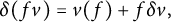 $$\begin{align*}\delta (fv) = v(f) + f\delta v,\end{align*}$$
for all
 $v\in \Gamma (\mathbb {T}M)$
,
$v\in \Gamma (\mathbb {T}M)$
,
 $f\in C^{\infty } (M)$
.
$f\in C^{\infty } (M)$
.
Example 2.12 Let D be a generalized connection on M. Then
 $$\begin{align*}\delta_Dv = \operatorname{\mathrm{tr}} Dv,\quad v\in \Gamma (\mathbb{T}M),\end{align*}$$
defines a divergence operator on
 $\mathbb {T}M$
.
$\mathbb {T}M$
.
When
 $M=G$
is a Lie group we can ask for a divergence operator
$M=G$
is a Lie group we can ask for a divergence operator
 $\delta $
on
$\delta $
on
 $\mathbb {T}G$
to be left-invariant, that is, for the function
$\mathbb {T}G$
to be left-invariant, that is, for the function
 $\delta v$
to be left-invariant (i.e., constant) for all left-invariant sections v of
$\delta v$
to be left-invariant (i.e., constant) for all left-invariant sections v of
 $\mathbb {T}G$
. Such operators can can be identified with elements of
$\mathbb {T}G$
. Such operators can can be identified with elements of
 $E^*=(\mathbb {T}_eG)^*$
.
$E^*=(\mathbb {T}_eG)^*$
.
It was proved in [Reference García FernándezG] that there always exists a Levi-Civita generalized connection with a prescribed divergence. We now give a proof for this in our setting.
Proposition 2.13 Let
 $(G,H,\mathcal G)$
be a generalized pseudo-Riemannian Lie group of dimension
$(G,H,\mathcal G)$
be a generalized pseudo-Riemannian Lie group of dimension
 $\dim G\ge 2$
and
$\dim G\ge 2$
and
 $\delta \in E^*$
. Then there exists a left-invariant Levi-Civita generalized connection D such that
$\delta \in E^*$
. Then there exists a left-invariant Levi-Civita generalized connection D such that
 $\delta _D=\delta $
.
$\delta _D=\delta $
.
Proof Let
 $D\in E^*\otimes \mathfrak {so}(E)$
be a left-invariant Levi-Civita generalized connection. Any other left-invariant Levi-Civita generalized connection can be written as
$D\in E^*\otimes \mathfrak {so}(E)$
be a left-invariant Levi-Civita generalized connection. Any other left-invariant Levi-Civita generalized connection can be written as
 $D'=D + S$
, where
$D'=D + S$
, where
 $S\in \mathfrak {so}(E)^{\langle 1\rangle }\subset E^*\otimes \mathfrak {so}(E)$
(see Proposition 2.8). The divergence operators are related by
$S\in \mathfrak {so}(E)^{\langle 1\rangle }\subset E^*\otimes \mathfrak {so}(E)$
(see Proposition 2.8). The divergence operators are related by
 $$ \begin{align} \delta_{D'}v - \delta_Dv = \operatorname{\mathrm{tr}} S v = \operatorname{\mathrm{tr}} (u\mapsto S_uv),\quad v\in E.\end{align} $$
We consider the linear form
 $\lambda _S \in E^*$
defined by
$\lambda _S \in E^*$
defined by
It suffices to show that the linear map
 $S \mapsto \lambda _S$
is surjective. Given
$S \mapsto \lambda _S$
is surjective. Given
 $\alpha , \beta \in E_+^*\cong (E_-)^0\subset E^*$
, the element
$\alpha , \beta \in E_+^*\cong (E_-)^0\subset E^*$
, the element
 $S=\mathrm {alt} (\alpha ^2 \otimes \beta )\in \Sigma _+ \subset \mathfrak {so}(E)^{\langle 1\rangle }=\Sigma _+\oplus \Sigma _-$
has
$S=\mathrm {alt} (\alpha ^2 \otimes \beta )\in \Sigma _+ \subset \mathfrak {so}(E)^{\langle 1\rangle }=\Sigma _+\oplus \Sigma _-$
has
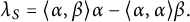 $$ \begin{align} \lambda_S = \langle \alpha,\beta \rangle \alpha -\langle \alpha ,\alpha\rangle \beta.\end{align} $$
Since
 $\dim E_+=\dim G\ge 2$
, this proves that
$\dim E_+=\dim G\ge 2$
, this proves that
 $\mathrm {span}\{ \lambda _S \mid S\in \Sigma _+\}=E_+^*$
, and similarly
$\mathrm {span}\{ \lambda _S \mid S\in \Sigma _+\}=E_+^*$
, and similarly
 $\mathrm {span}\{ \lambda _S \mid S\in \Sigma _-\}=E_-^*$
.
$\mathrm {span}\{ \lambda _S \mid S\in \Sigma _-\}=E_-^*$
.
Note that the condition
 $\dim G\ge 2$
is necessary. If
$\dim G\ge 2$
is necessary. If
 $\dim G =1$
, then the Levi-Civita generalized connection D is unique and
$\dim G =1$
, then the Levi-Civita generalized connection D is unique and
 $\delta _D\in E^*$
is zero.
$\delta _D\in E^*$
is zero.
From now on, we assume without loss of generality (see Proposition 2.4) that
 $\mathcal G = \mathcal G_g$
for some left-invariant pseudo-Riemannian metric g on G. We will first construct a particular left-invariant Levi-Civita generalized connection D with
$\mathcal G = \mathcal G_g$
for some left-invariant pseudo-Riemannian metric g on G. We will first construct a particular left-invariant Levi-Civita generalized connection D with
 $\delta _D=0\in E^*$
and later prescribe an arbitrary divergence operator by adding a suitable element of the generalized first prolongation.
$\delta _D=0\in E^*$
and later prescribe an arbitrary divergence operator by adding a suitable element of the generalized first prolongation.
Adapted bases and notation
Let
 $(v_a)=(v_1,\ldots ,v_n)$
be a g-orthonormal basis of
$(v_a)=(v_1,\ldots ,v_n)$
be a g-orthonormal basis of
 $\mathfrak {g}$
and set
$\mathfrak {g}$
and set
![]() . Then
. Then
defines a
 $\mathcal G$
-orthonormal basis
$\mathcal G$
-orthonormal basis
 $(e_a)_{a=1,\ldots ,n}$
of
$(e_a)_{a=1,\ldots ,n}$
of
 $E_+$
with
$E_+$
with
 $\mathcal {G}(e_a,e_a) = \varepsilon _a$
and
$\mathcal {G}(e_a,e_a) = \varepsilon _a$
and
defines a
 $\mathcal G$
-orthonormal basis
$\mathcal G$
-orthonormal basis
 $(e_i)_{i=n+1,\ldots ,2n}$
of
$(e_i)_{i=n+1,\ldots ,2n}$
of
 $E_-$
with
$E_-$
with
 $\mathcal {G}(e_{n+a},e_{n+a}) = \varepsilon _{a}$
. Remember that
$\mathcal {G}(e_{n+a},e_{n+a}) = \varepsilon _{a}$
. Remember that
 $\langle \cdot ,\cdot \rangle = \pm \mathcal G$
on the summands
$\langle \cdot ,\cdot \rangle = \pm \mathcal G$
on the summands
 $E_{\pm }$
of the decomposition
$E_{\pm }$
of the decomposition
 $E=E_+ \oplus E_-$
, which is orthogonal for both the generalized metric
$E=E_+ \oplus E_-$
, which is orthogonal for both the generalized metric
 $\mathcal G$
as well as the scalar product
$\mathcal G$
as well as the scalar product
 $\langle \cdot ,\cdot \rangle $
. Summarizing, we have an orthonormal basis
$\langle \cdot ,\cdot \rangle $
. Summarizing, we have an orthonormal basis
 $(e_A)_{A=1,\ldots ,2n}$
of E adapted to the decomposition
$(e_A)_{A=1,\ldots ,2n}$
of E adapted to the decomposition
 $E=E_+\oplus E_-$
. Note that
$E=E_+\oplus E_-$
. Note that
 $\langle e_A,e_B\rangle = \varepsilon _A\delta _{AB}$
, where
$\langle e_A,e_B\rangle = \varepsilon _A\delta _{AB}$
, where
 $\varepsilon _a = -\varepsilon _{n+a}$
for
$\varepsilon _a = -\varepsilon _{n+a}$
for
 $a=1,\ldots , n$
. From now on the indices
$a=1,\ldots , n$
. From now on the indices
 $a, b, \ldots $
will always range from
$a, b, \ldots $
will always range from
 $1$
to n,
$1$
to n,
 $i, j, \ldots $
will range from
$i, j, \ldots $
will range from
 $n+1$
to
$n+1$
to
 $2n$
and
$2n$
and
 $A, B, \ldots $
from
$A, B, \ldots $
from
 $1$
to
$1$
to
 $2n$
.
$2n$
.
A left-invariant generalized connection D is completely determined by its coefficients
 $\omega _{AB}^C$
with respect to the basis
$\omega _{AB}^C$
with respect to the basis
 $(e_A)$
:
$(e_A)$
:
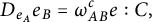 $$\begin{align*}D_{e_A}e_B= \omega_{AB}^ce:C,\end{align*}$$
where, from now on, we use Einstein’s summation convention, according to which the sum over an upper and a lower repeated index is understood. Equivalently, we may use
which has the advantage that it is skew-symmetric in
 $(B,C)$
. In fact, any tensor
$(B,C)$
. In fact, any tensor
 $(\omega _{ABC})$
skew-symmetric in
$(\omega _{ABC})$
skew-symmetric in
 $(B,C)$
defines a left-invariant generalized connection D by the formula (15). We will say that
$(B,C)$
defines a left-invariant generalized connection D by the formula (15). We will say that
 $(\omega _{ABC})$
are the connection coefficients of D.
$(\omega _{ABC})$
are the connection coefficients of D.
The next proposition follows from the fact that D is metric if and only if
 $DE_{\pm }\subset E_{\pm }$
.
$DE_{\pm }\subset E_{\pm }$
.
Proposition 2.14 A left-invariant generalized connection D is metric if and only if
 $\omega _{ABC}=0$
whenever
$\omega _{ABC}=0$
whenever
 $B\in \{1,\ldots ,n\}$
and
$B\in \{1,\ldots ,n\}$
and
 $C\in \{ n+1,\ldots ,2n\}$
.
$C\in \{ n+1,\ldots ,2n\}$
.
Using the orthonormal basis
 $(e_A)$
of E, we define
$(e_A)$
of E, we define
Proposition 2.15 Let
 $(G,H,\mathcal G_g)$
be a generalized pseudo-Riemannian Lie group. The following tensor
$(G,H,\mathcal G_g)$
be a generalized pseudo-Riemannian Lie group. The following tensor
 $(\omega _{ABC})$
defines the connection coefficients of a left-invariant Levi-Civita generalized connection
$(\omega _{ABC})$
defines the connection coefficients of a left-invariant Levi-Civita generalized connection
 $D^0$
with zero divergence
$D^0$
with zero divergence
 $\delta _{D^0}$
:
$\delta _{D^0}$
:
where
 $a,b,c\in \{ 1,\ldots ,n\}$
and
$a,b,c\in \{ 1,\ldots ,n\}$
and
 $i,j,k\in \{ n+1,\ldots ,2n\}$
and the remaining components are zero. The connection
$i,j,k\in \{ n+1,\ldots ,2n\}$
and the remaining components are zero. The connection
 $D^0$
does not depend on the choice of orthonormal basis
$D^0$
does not depend on the choice of orthonormal basis
 $(v_a)$
of
$(v_a)$
of
 $\mathfrak {g}$
, from which the orthonormal basis
$\mathfrak {g}$
, from which the orthonormal basis
 $(e_A)$
of
$(e_A)$
of
 $E=\mathfrak {g}\oplus \mathfrak {g}^*$
was constructed. It is therefore a canonical Levi-Civita generalized connection and will be called the canonical divergence-free Levi-Civita generalized connection.
$E=\mathfrak {g}\oplus \mathfrak {g}^*$
was constructed. It is therefore a canonical Levi-Civita generalized connection and will be called the canonical divergence-free Levi-Civita generalized connection.
Proof The formulas (17) are precisely the connection coefficients of the left-invariant Levi-Civita generalized connection
 $D^0$
defined in the proof of Proposition 2.8. In particular,
$D^0$
defined in the proof of Proposition 2.8. In particular,
 $D^0$
is independent of the basis
$D^0$
is independent of the basis
 $(v_a)$
. To show that the divergence
$(v_a)$
. To show that the divergence
 $\delta $
of
$\delta $
of
 $D^0$
vanishes, it suffices to remark that
$D^0$
vanishes, it suffices to remark that
 $\delta (e_B) = \omega _{AB}^A$
vanishes due to
$\delta (e_B) = \omega _{AB}^A$
vanishes due to
 $\omega _{ajc}=\omega _{ibk}=0$
and the total skew-symmetry of
$\omega _{ajc}=\omega _{ibk}=0$
and the total skew-symmetry of
 $\omega _{abc}$
and
$\omega _{abc}$
and
 $\omega _{ijk}$
(with the above index ranges), implied by Lemma 2.9.
$\omega _{ijk}$
(with the above index ranges), implied by Lemma 2.9.
Proposition 2.16 Let
 $(G,H,\mathcal G_g)$
be a generalized pseudo-Riemannian Lie group endowed with the canonical divergence-free Levi-Civita generalized connection
$(G,H,\mathcal G_g)$
be a generalized pseudo-Riemannian Lie group endowed with the canonical divergence-free Levi-Civita generalized connection
 $D^0$
of Proposition 2.15. Fix an element
$D^0$
of Proposition 2.15. Fix an element
 $\delta \in E^*$
. Then a left-invariant Levi-Civita generalized connection D with divergence
$\delta \in E^*$
. Then a left-invariant Levi-Civita generalized connection D with divergence
 $\delta _D=\delta $
can be obtained as follows. Choose, as above,Footnote
1
a left-invariant orthonormal basis
$\delta _D=\delta $
can be obtained as follows. Choose, as above,Footnote
1
a left-invariant orthonormal basis
 $(e_A)$
of E associated with an orthonormal basis of
$(e_A)$
of E associated with an orthonormal basis of
 $\mathfrak g$
. Define the tensor
$\mathfrak g$
. Define the tensor
 $ S:=S_+ +S_-$
, where
$ S:=S_+ +S_-$
, where
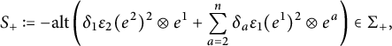
and similarly for
 $ S_- \in \Sigma _-$
. Here,
$ S_- \in \Sigma _-$
. Here,
 $(e^A)$
denotes the basis of
$(e^A)$
denotes the basis of
 $E^*$
dual to
$E^*$
dual to
 $(e_A)$
and
$(e_A)$
and
 $\delta _A = \delta (e_A)$
. Then the left-invariant Levi-Civita generalized connection
$\delta _A = \delta (e_A)$
. Then the left-invariant Levi-Civita generalized connection
 $D=D^0 +S$
has divergence
$D=D^0 +S$
has divergence
 $\delta $
.
$\delta $
.
Proof From (10)–(12), we see that
 $D=D^0 + S$
has divergence
$D=D^0 + S$
has divergence
 $ \delta $
, since
$ \delta $
, since
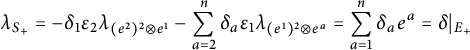 $$\begin{align*}\lambda_{S_+} = -\delta_1 \varepsilon_2\lambda_{(e^2)^2 \otimes e^1} -\sum_{a=2}^{n}\delta_a\varepsilon_1\lambda_{(e^1)^2\otimes e^a}=\sum_{a=1}^{n}\delta_ae^a=\delta|_{E_+}\end{align*}$$
and similarly
 $ \lambda _{S_-}=\delta |_{E_-} $
.
$ \lambda _{S_-}=\delta |_{E_-} $
.
We want to close this section by introducing a special divergence operator, the so-called Riemannian divergence, which is considered in the literature ([Reference García Fernández and StreetsGSt, Definition 2.46]). If
 $ (M,\mathcal {G}) $
is a generalized pseudo-Riemannian manifold, one defines for all
$ (M,\mathcal {G}) $
is a generalized pseudo-Riemannian manifold, one defines for all
 $v\in \Gamma (\mathbb {T}M),$
 $$ \begin{align*} \delta^{\mathcal{G}}(v)= \operatorname{\mathrm{tr}} \left(\nabla \pi v\right)=\operatorname{\mathrm{tr}}\left(\Gamma(TM)\ni Y \mapsto \nabla_Y\pi(v)\in \Gamma(TM)\right), \end{align*} $$
where
 $ \nabla $
is the Levi-Civita connection of the pseudo-Riemannian metric
$ \nabla $
is the Levi-Civita connection of the pseudo-Riemannian metric
 $ g $
associated with
$ g $
associated with
 $ \mathcal {G} $
via Proposition 2.4. Denoting by
$ \mathcal {G} $
via Proposition 2.4. Denoting by
 $ \mu $
the Riemannian density associated with
$ \mu $
the Riemannian density associated with
 $ g $
, we recall the well-known fact that the divergence
$ g $
, we recall the well-known fact that the divergence
 $\operatorname {\mathrm{tr}} \left (\nabla X\right )$
of a vector field X can also be expressed by
$\operatorname {\mathrm{tr}} \left (\nabla X\right )$
of a vector field X can also be expressed by
 $\frac {\mathcal {L}_X \mu }{\mu }$
, since
$\frac {\mathcal {L}_X \mu }{\mu }$
, since
 $$ \begin{align*} \mathcal{L}_X \mu = \nabla_X\mu -(\nabla X) \cdot \mu = \operatorname{\mathrm{tr}} (\nabla X)\mu. \end{align*} $$
The divergence operator
 $\delta ^{\mathcal {G}}$
can be recovered as the divergence of a generalized connection as in Example 2.12. For that one, first extends the Levi-Civita connection to a connection on
$\delta ^{\mathcal {G}}$
can be recovered as the divergence of a generalized connection as in Example 2.12. For that one, first extends the Levi-Civita connection to a connection on
 $ \mathbb {T}M $
and then pulls it back to a generalized connection
$ \mathbb {T}M $
and then pulls it back to a generalized connection
 $ \widetilde {\nabla } $
via the anchor
$ \widetilde {\nabla } $
via the anchor
 $\pi $
. Then
$\pi $
. Then
 $$ \begin{align*} \delta_{\widetilde{\nabla}}(v)=\operatorname{\mathrm{tr}}_{\mathbb{T}M}\left(\widetilde{\nabla}v\right)=\operatorname{\mathrm{tr}}_{TM}\left(\nabla\pi(v)\right)=\delta^{\mathcal{G}}(v), \end{align*} $$
since
 $ \widetilde {\nabla }v|_{T^*M}=0 $
and
$ \widetilde {\nabla }v|_{T^*M}=0 $
and
 $ \pi \circ \widetilde {\nabla }v|_{TM}=\nabla \pi (v)$
. Furthermore, note that
$ \pi \circ \widetilde {\nabla }v|_{TM}=\nabla \pi (v)$
. Furthermore, note that
 $ \widetilde {\nabla } $
is a Levi-Civita generalized connection of
$ \widetilde {\nabla } $
is a Levi-Civita generalized connection of
 $ \mathcal {G} $
, if
$ \mathcal {G} $
, if
 $ \mathcal {G}=\mathcal {G}^g $
and
$ \mathcal {G}=\mathcal {G}^g $
and
 $H=0$
.
$H=0$
.
Proposition 2.17 Let
 $(G, H,\mathcal G)$
be a generalized pseudo-Riemannian Lie group. Then the Riemannian divergence satisfies
$(G, H,\mathcal G)$
be a generalized pseudo-Riemannian Lie group. Then the Riemannian divergence satisfies
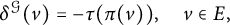 $$ \begin{align*} \delta^{\mathcal{G}}(v)=-\tau(\pi(v)), \quad v\in E, \end{align*} $$
where
 $\tau \in \mathfrak {g}^*$
is the trace-form defined by
$\tau \in \mathfrak {g}^*$
is the trace-form defined by
 $\tau (X) = \operatorname {\mathrm{tr}} \mathrm {ad}_{X}$
,
$\tau (X) = \operatorname {\mathrm{tr}} \mathrm {ad}_{X}$
,
 $X\in \mathfrak {g}$
. In particular, the Riemannian divergence is zero, if the Lie group
$X\in \mathfrak {g}$
. In particular, the Riemannian divergence is zero, if the Lie group
 $ G $
is unimodular.
$ G $
is unimodular.
Proof Let
 $ v=X+\xi \in E $
and
$ v=X+\xi \in E $
and
 $ (v_a) $
as usual a basis of
$ (v_a) $
as usual a basis of
 $ \mathfrak {g} $
, which is orthonormal with respect to
$ \mathfrak {g} $
, which is orthonormal with respect to
 $ g $
. Furthermore, let
$ g $
. Furthermore, let
 $ \nabla $
be the Levi-Civita connection of
$ \nabla $
be the Levi-Civita connection of
 $ g $
. It satisfies
$ g $
. It satisfies
 $$ \begin{align*} g\left(\nabla_XY,Z\right)=\frac12\left(g\left([X,Y],Z\right)-g\left([Y,Z],X\right)+g\left([Z,X],Y\right)\right) \end{align*} $$
for
 $ X,Y,Z\in \mathfrak {g} $
. We can thus compute
$ X,Y,Z\in \mathfrak {g} $
. We can thus compute
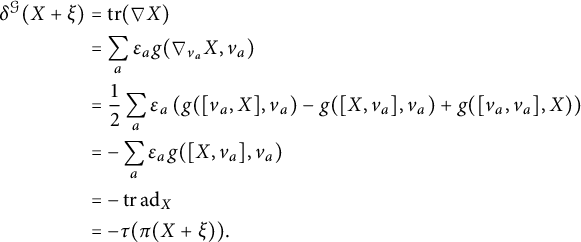 $$ \begin{align*} \delta^{\mathcal{G}}(X+\xi)&=\operatorname{\mathrm{tr}}(\nabla X)\\ &=\sum_a\varepsilon_ag(\nabla_{v_a}X,v_a)\\ &=\frac12\sum_a\varepsilon_a\left(g([v_a,X],v_a)-g([X,v_a],v_a)+g([v_a,v_a],X)\right)\\ &=-\sum_a\varepsilon_ag([X,v_a],v_a)\\ &=-\operatorname{\mathrm{tr}}\mathrm{ad}_X\\ &=-\tau(\pi(X+\xi)).\\[-35pt] \end{align*} $$
2.5 Ricci curvatures and generalized Einstein metrics
After fixing a left-invariant section
 $\delta $
of
$\delta $
of
 $(\mathbb {T}G)^*$
over a generalized pseudo-Riemannian Lie group
$(\mathbb {T}G)^*$
over a generalized pseudo-Riemannian Lie group
 $(G,H,\mathcal G)$
we define and compute two canonical Ricci curvature tensors
$(G,H,\mathcal G)$
we define and compute two canonical Ricci curvature tensors
 $Ric^+\in E_-^*\otimes E_+^*$
and
$Ric^+\in E_-^*\otimes E_+^*$
and
 $Ric^-\in E_+^*\otimes E_-^*$
, which depend only on the data
$Ric^-\in E_+^*\otimes E_-^*$
, which depend only on the data
 $(H,\mathcal G,\delta )$
. A left-invariant solution
$(H,\mathcal G,\delta )$
. A left-invariant solution
 $\mathcal {G}$
of the system
$\mathcal {G}$
of the system
 $Ric^+=0, Ric^-=0$
is what we will call a generalized Einstein metric on G with three-form H and dilaton
$Ric^+=0, Ric^-=0$
is what we will call a generalized Einstein metric on G with three-form H and dilaton
 $\delta $
.
$\delta $
.
Consider the generalized tangent bundle
 $\mathbb {T}M$
of a smooth manifold endowed with the Courant algebroid structure associated with a closed three-form H on M and a generalized pseudo-Riemannian metric
$\mathbb {T}M$
of a smooth manifold endowed with the Courant algebroid structure associated with a closed three-form H on M and a generalized pseudo-Riemannian metric
 $\mathcal G$
. We denote by
$\mathcal G$
. We denote by
 $(\mathbb {T}M)_{\pm }$
the eigenbundles of
$(\mathbb {T}M)_{\pm }$
the eigenbundles of
 $\mathcal G^{\mathrm {end}}$
.
$\mathcal G^{\mathrm {end}}$
.
Given a Levi-Civita generalized connection D on
 $\mathbb {T}M$
and two sections
$\mathbb {T}M$
and two sections
 $u,v\in \Gamma (\mathbb {T}M)$
, we consider the differential operator
$u,v\in \Gamma (\mathbb {T}M)$
, we consider the differential operator
 $R(u,v): \Gamma (\mathbb {T}M)\rightarrow \Gamma (\mathbb {T}M)$
defined by
$R(u,v): \Gamma (\mathbb {T}M)\rightarrow \Gamma (\mathbb {T}M)$
defined by
for all
 $w\in \Gamma (\mathbb {T}M)$
. It was observed in [Reference García FernándezG] that R restricts to tensor fields
$w\in \Gamma (\mathbb {T}M)$
. It was observed in [Reference García FernándezG] that R restricts to tensor fields
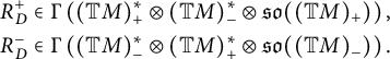 $$ \begin{align*} R_D^+&\in \Gamma \left((\mathbb{T}M)_+^*\otimes (\mathbb{T}M)_-^*\otimes \mathfrak{so}((\mathbb{T}M)_+)\right),\\ R_D^-&\in \Gamma \left((\mathbb{T}M)_-^*\otimes (\mathbb{T}M)_+^*\otimes \mathfrak{so}((\mathbb{T}M)_-)\right). \end{align*} $$
Hence there are tensor fields
 $Ric_D^+\in \Gamma ((\mathbb {T}M)_-^*\otimes (\mathbb {T}M)_+^*)$
and
$Ric_D^+\in \Gamma ((\mathbb {T}M)_-^*\otimes (\mathbb {T}M)_+^*)$
and
 $Ric_D^-\in \Gamma ((\mathbb {T}M)_+^*\otimes (\mathbb {T}M)_-^*)$
defined by
$Ric_D^-\in \Gamma ((\mathbb {T}M)_+^*\otimes (\mathbb {T}M)_-^*)$
defined by
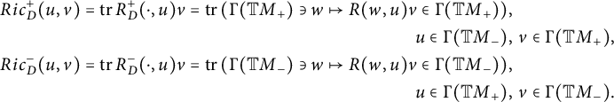 $$ \begin{align*} \begin{aligned} Ric_D^+(u,v) = \operatorname{\mathrm{tr}} R_D^+(\cdot , u)v = \operatorname{\mathrm{tr}} \left(\Gamma({\mathbb{T}M}_+)\ni w\mapsto R(w,u)v\in \Gamma({\mathbb{T}M}_+)\right)&,\\ u\in \Gamma({\mathbb{T}M}_-)&, \, v\in \Gamma({\mathbb{T}M}_+),\\ Ric_D^-(u,v) = \operatorname{\mathrm{tr}} R_D^-(\cdot , u)v = \operatorname{\mathrm{tr}} \left(\Gamma({\mathbb{T}M}_-)\ni w\mapsto R(w,u)v\in \Gamma({\mathbb{T}M}_-)\right)&,\\ u\in \Gamma({\mathbb{T}M}_+)&, \, v\in \Gamma({\mathbb{T}M}_-). \end{aligned} \end{align*} $$
It was also shown in [Reference García FernándezG] that the tensor fields
 $Ric_{D_1}^{\pm }$
and
$Ric_{D_1}^{\pm }$
and
 $Ric_{D_2}^{\pm }$
are the same for any pair of Levi-Civita generalized connections
$Ric_{D_2}^{\pm }$
are the same for any pair of Levi-Civita generalized connections
 $D_1$
,
$D_1$
,
 $D_2$
with the same divergence operator
$D_2$
with the same divergence operator
 $\delta _{D_1}=\delta _{D_2}$
.
$\delta _{D_1}=\delta _{D_2}$
.
As a consequence, the following definition is meaningful.
Definition 2.18 Let
 $(G,H,\mathcal G)$
be a generalized pseudo-Riemannian Lie group and
$(G,H,\mathcal G)$
be a generalized pseudo-Riemannian Lie group and
 $\delta \in E^*$
. Then the Ricci curvatures
$\delta \in E^*$
. Then the Ricci curvatures
 $$\begin{align*}Ric^+=Ric^+_{\delta}\in E_-^*\otimes E_+^*\quad\mbox{and}\quad Ric^-=Ric^-_{\delta}\in E_+^*\otimes E_-^*\\[-9pt]\end{align*}$$
of
 $(G,H,\mathcal G, \delta )$
(or of
$(G,H,\mathcal G, \delta )$
(or of
 $(\mathfrak {g},H,\mathcal G, \delta )$
) are defined by evaluation of
$(\mathfrak {g},H,\mathcal G, \delta )$
) are defined by evaluation of
 $Ric_D^+$
and
$Ric_D^+$
and
 $Ric_D^-$
at
$Ric_D^-$
at
 $e\in G$
, where D is any left-invariant Levi-Civita generalized connection D with divergence
$e\in G$
, where D is any left-invariant Levi-Civita generalized connection D with divergence
 $\delta $
.
$\delta $
.
 $(G,H,\mathcal G, \delta )$
is called generalized Einstein if
$(G,H,\mathcal G, \delta )$
is called generalized Einstein if
We will consider
 $Ric$
as a bilinear form on E vanishing on
$Ric$
as a bilinear form on E vanishing on
 $E_+\times E_+$
and
$E_+\times E_+$
and
 $E_-\times E_-$
.
$E_-\times E_-$
.
Next, we compute the Ricci curvatures in the case
 $\delta =0$
using the canonical divergence-free Levi-Civita generalized connection of Proposition 2.15, which in the following we denote by
$\delta =0$
using the canonical divergence-free Levi-Civita generalized connection of Proposition 2.15, which in the following we denote by
 $D^0$
. The case of general divergence is then obtained by computing how the Ricci curvatures change under addition of an element of the generalized first prolongation. We denote by
$D^0$
. The case of general divergence is then obtained by computing how the Ricci curvatures change under addition of an element of the generalized first prolongation. We denote by
 $R^{\pm }_{D^0}\in E_{\pm }^*\otimes E_{\mp }^*\otimes \mathfrak {so}(E_{\pm })$
the tensors which correspond to the left-invariant tensor fields
$R^{\pm }_{D^0}\in E_{\pm }^*\otimes E_{\mp }^*\otimes \mathfrak {so}(E_{\pm })$
the tensors which correspond to the left-invariant tensor fields
 $R^{\pm }_{D^0}\in \Gamma \left ( (\mathbb {T}G)_{\pm }^*\otimes (\mathbb {T}G)_{\mp }^*\otimes \mathfrak {so}((\mathbb {T}G)_{\pm })\right )$
.
$R^{\pm }_{D^0}\in \Gamma \left ( (\mathbb {T}G)_{\pm }^*\otimes (\mathbb {T}G)_{\mp }^*\otimes \mathfrak {so}((\mathbb {T}G)_{\pm })\right )$
.
Proposition 2.19 Let
 $D^0$
be the canonical divergence-free Levi-Civita generalized connection of a generalized pseudo-Riemannian Lie group
$D^0$
be the canonical divergence-free Levi-Civita generalized connection of a generalized pseudo-Riemannian Lie group
 $(G,H,\mathcal G_g)$
, defined in Proposition 2.15. The components
$(G,H,\mathcal G_g)$
, defined in Proposition 2.15. The components
![]() ,
,
 $A,B,C,D\in \{ 1,\ldots ,2n\}$
, of the tensors
$A,B,C,D\in \{ 1,\ldots ,2n\}$
, of the tensors
 $R^{\pm }_{D^0}$
are given by
$R^{\pm }_{D^0}$
are given by
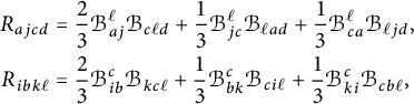 $$ \begin{align*} R_{ajcd} &= \frac23 \mathcal{B}_{aj}^{\ell} \mathcal{B}_{c\ell d} +\frac13 \mathcal{B}_{jc}^{\ell} \mathcal{B}_{\ell a d} +\frac13 \mathcal{B}_{ca}^{\ell} \mathcal{B}_{\ell j d},\\ R_{ibk\ell } &= \frac23 \mathcal{B}_{ib}^c \mathcal{B}_{kc \ell} +\frac13 \mathcal{B}_{bk}^c\mathcal{B}_{ci\ell } +\frac13 \mathcal{B}_{ki}^c\mathcal{B}_{cb\ell },\\[-9pt] \end{align*} $$
where
 $a,b,c,d\in \{ 1,\ldots ,n\}$
and
$a,b,c,d\in \{ 1,\ldots ,n\}$
and
 $i,j,k,\ell \in \{ n+1,\ldots ,2n\}$
.
$i,j,k,\ell \in \{ n+1,\ldots ,2n\}$
.
Proof We denote by
 $\eta _{AB} =\langle e_A,e_B\rangle $
the coefficients of the scalar product with respect to the orthonormal basis
$\eta _{AB} =\langle e_A,e_B\rangle $
the coefficients of the scalar product with respect to the orthonormal basis
 $(e_A)$
and by
$(e_A)$
and by
 $\omega _{ABC}$
and
$\omega _{ABC}$
and
 $\omega _{AB}^C=\sum _{D} \eta ^{CD} \omega _{ABD}$
the connection coefficients of
$\omega _{AB}^C=\sum _{D} \eta ^{CD} \omega _{ABD}$
the connection coefficients of
 $D^0$
. Here,
$D^0$
. Here,
 $\eta ^{AB}=\eta _{AB}$
are the coefficients of the induced scalar product on
$\eta ^{AB}=\eta _{AB}$
are the coefficients of the induced scalar product on
 $E^*$
. Then (taking into account the agreed index ranges) we compute
$E^*$
. Then (taking into account the agreed index ranges) we compute
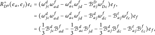 $$ \begin{align*} R_{D^0}^+(e_a,e_j)e_c&=(\omega_{jc}^d\omega_{ad}^f -\omega_{ac}^d\omega_{jd}^f - \mathcal{B}_{aj}^D\omega_{Dc}^f)e_f,\\ &=(\omega_{jc}^d\omega_{ad}^f -\omega_{ac}^d\omega_{jd}^f - \mathcal{B}_{aj}^d\omega_{dc}^f- \mathcal{B}_{aj}^{\ell} \omega_{\ell c}^f)e_f\\ &=(\frac13 \mathcal{B}_{jc}^d\mathcal{B}_{ad}^f -\frac13 \mathcal{B}_{ac}^d\mathcal{B}_{jd}^f - \frac13 \mathcal{B}_{aj}^d\mathcal{B}_{dc}^f- \mathcal{B}_{aj}^{\ell} \mathcal{B}_{\ell c}^f)e_f,\\[-9pt] \end{align*} $$
where the index f runs from
 $1$
to n and
$1$
to n and
 $\mathcal {B}_{AB}^C=\mathcal {B}_{ABD}\eta ^{DC}$
. Next, we observe that the axiom (C1), the Jacobi identity for the Dorfman bracket, can be written in components as
$\mathcal {B}_{AB}^C=\mathcal {B}_{ABD}\eta ^{DC}$
. Next, we observe that the axiom (C1), the Jacobi identity for the Dorfman bracket, can be written in components as
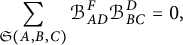 $$\begin{align*}\sum_{\mathfrak{S}(A,B,C)} \mathcal{B}_{AD}^F\mathcal{B}_{BC}^D=0,\\[-9pt]\end{align*}$$
where the cyclic sum is over
 $(A,B,C)$
. Specializing to
$(A,B,C)$
. Specializing to
 $(A,B,C,F)=(a,j,c,f),$
we get
$(A,B,C,F)=(a,j,c,f),$
we get
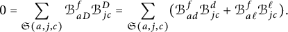 $$\begin{align*}0=\sum_{\mathfrak{S}(a,j,c)} \mathcal{B}_{aD}^f\mathcal{B}_{jc}^D=\sum_{\mathfrak{S}(a,j,c)}(\mathcal{B}_{ad}^f\mathcal{B}_{jc}^d +\mathcal{B}_{a\ell }^f\mathcal{B}_{jc}^{\ell} ).\\[-9pt]\end{align*}$$
So we obtain
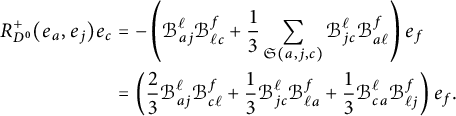 $$ \begin{align*} R_{D^0}^+(e_a,e_j)e_c&= -\left( \mathcal{B}_{aj}^{\ell} \mathcal{B}_{\ell c}^f +\frac13 \sum_{\mathfrak{S}(a,j,c)} \mathcal{B}_{jc}^{\ell} \mathcal{B}_{a\ell }^f \right) e_f\\ &=\left( \frac23 \mathcal{B}_{aj}^{\ell} \mathcal{B}_{c\ell }^f +\frac13 \mathcal{B}_{jc}^{\ell} \mathcal{B}_{\ell a}^f +\frac13 \mathcal{B}_{ca}^{\ell} \mathcal{B}_{\ell j}^f\right) e_f. \\[-9pt]\end{align*} $$
Taking the scalar product with
 $e_d$
gives the claimed formula for
$e_d$
gives the claimed formula for
 $R_{ajcd}$
. The other formula is obtained similarly.
$R_{ajcd}$
. The other formula is obtained similarly.
Corollary 2.20 Let
 $(G,H,\mathcal G_g)$
be a generalized pseudo-Riemannian Lie group. Then the Ricci curvature of
$(G,H,\mathcal G_g)$
be a generalized pseudo-Riemannian Lie group. Then the Ricci curvature of
 $(G,H,\mathcal G_g,\delta =0)$
is symmetric, in the sense that
$(G,H,\mathcal G_g,\delta =0)$
is symmetric, in the sense that
 $Ric^+(u,v)=Ric^-(v,u)$
for all
$Ric^+(u,v)=Ric^-(v,u)$
for all
 $u\in E_-$
,
$u\in E_-$
,
 $v\in E_+$
. The components
$v\in E_+$
. The components
![]() of
of
 $Ric^+$
are given by
$Ric^+$
are given by
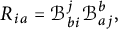 $$\begin{align*}R_{ia} = \mathcal{B}_{bi}^j \mathcal{B}_{aj}^b,\\[-9pt] \end{align*}$$
where
 $a,b\in \{ 1,\ldots ,n\}$
and
$a,b\in \{ 1,\ldots ,n\}$
and
 $i,j\in \{ n+1,\ldots ,2n\}$
.
$i,j\in \{ n+1,\ldots ,2n\}$
.
Proof From Proposition 2.19, by taking the trace using the complete skew-symmetry of
 $\mathcal {B}_{ABC}$
(see Lemma 2.9), we get
$\mathcal {B}_{ABC}$
(see Lemma 2.9), we get
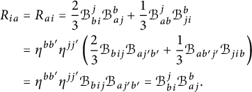 $$ \begin{align*} R_{ia} &= R_{ai}= \frac23 \mathcal{B}_{bi}^j \mathcal{B}_{aj}^b +\frac13 \mathcal{B}_{ab}^j \mathcal{B}_{j i}^b\\ &= \eta^{bb'} \eta^{jj'}\left( \frac23 \mathcal{B}_{bij} \mathcal{B}_{aj'b'} +\frac13 \mathcal{B}_{ab'j'} \mathcal{B}_{j ib}\right)\\ &= \eta^{bb'} \eta^{jj'} \mathcal{B}_{bij} \mathcal{B}_{aj'b'} = \mathcal{B}_{bi}^j \mathcal{B}_{aj}^b.\\[-35pt] \end{align*} $$
For
 $u_{\pm } \in E_{\pm }$
, we define
$u_{\pm } \in E_{\pm }$
, we define
Corollary 2.21 A necessary and sufficient condition for
 $(G,H,\mathcal G_g,\delta =0)$
to be generalized Einstein is that the subspace
$(G,H,\mathcal G_g,\delta =0)$
to be generalized Einstein is that the subspace
 $$\begin{align*}\Gamma_{E_+} \subset \mathrm{Hom}(E_-,E_+)\quad \mbox{is perpendicular to}\quad \Gamma_{E_-} \subset \mathrm{Hom}(E_+,E_-),\end{align*}$$
with respect to the nondegenerate pairing
 $\mathrm {Hom}(E_-,E_+)\times \mathrm {Hom}(E_+,E_-)\rightarrow \mathbb {R}$
given by
$\mathrm {Hom}(E_-,E_+)\times \mathrm {Hom}(E_+,E_-)\rightarrow \mathbb {R}$
given by
 $(A,B) \mapsto \operatorname {\mathrm{tr}} (AB) = \operatorname {\mathrm{tr}} (BA)$
. A sufficient condition in terms of the subspaces
$(A,B) \mapsto \operatorname {\mathrm{tr}} (AB) = \operatorname {\mathrm{tr}} (BA)$
. A sufficient condition in terms of the subspaces
 $\Gamma _{E_{\pm }}E_{\mp } \subset E_{\pm }$
is that
$\Gamma _{E_{\pm }}E_{\mp } \subset E_{\pm }$
is that
 $$ \begin{align} \Gamma_{E_+}E_-\perp [E_-,E_-]_H\quad\mbox{or}\quad \Gamma_{E_-}E_+\perp [E_+,E_+]_H.\\[-9pt]\nonumber\end{align} $$
Proof The necessary and sufficient condition follows immediately from
 $$\begin{align*}R_{ia} = R_{ai}= \mathcal{B}_{bi}^j \mathcal{B}_{aj}^b=-\operatorname{\mathrm{tr}} (\Gamma_{e_a}\circ \Gamma_{e_i}).\\[-9pt]\end{align*}$$
Any of the two (nonequivalent) conditions
 $\Gamma _{E_+} \circ \Gamma _{E_-}=0$
or
$\Gamma _{E_+} \circ \Gamma _{E_-}=0$
or
 $\Gamma _{E_-} \circ \Gamma _{E_+}=0$
is clearly sufficient. These can be reformulated as (19), since, by Lemma 2.9,
$\Gamma _{E_-} \circ \Gamma _{E_+}=0$
is clearly sufficient. These can be reformulated as (19), since, by Lemma 2.9,
 $$\begin{align*}\langle \Gamma_{u_+}v_-,w_+\rangle = -\langle v_-,[u_+,w_+]_H\rangle\quad\mbox{and}\quad \langle \Gamma_{u_-}v_+,w_-\rangle = -\langle v_+,[u_-,w_-]_H\rangle,\end{align*}$$
for all
 $u_+,v_+, w_+\in E_+$
,
$u_+,v_+, w_+\in E_+$
,
 $u_-,v_-,w_-\in E_-$
.
$u_-,v_-,w_-\in E_-$
.
Next, we will compute the Ricci curvature of an arbitrary left-invariant Levi-Civita generalized connection
 $D=D^0 + S$
on
$D=D^0 + S$
on
 $(G,H,\mathcal G_g)$
, where
$(G,H,\mathcal G_g)$
, where
 $D^0$
is the canonical divergence-free Levi-Civita generalized connection and S is an arbitrary element of the first generalized prolongation of
$D^0$
is the canonical divergence-free Levi-Civita generalized connection and S is an arbitrary element of the first generalized prolongation of
 $\mathfrak {so}(E)$
.
$\mathfrak {so}(E)$
.
Lemma 2.22 The curvature tensors
 $R^{\pm }_D\in \mathrm {Hom}(E_{\pm } \otimes E_{\mp }\otimes E_{\pm },E_{\pm })$
of D are given by
$R^{\pm }_D\in \mathrm {Hom}(E_{\pm } \otimes E_{\mp }\otimes E_{\pm },E_{\pm })$
of D are given by
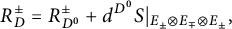 $$ \begin{align} R_{D}^{\pm} = R_{D^0}^{\pm} + d^{D^0}S|_{E_{\pm} \otimes E_{\mp}\otimes E_{\pm}},\\[-9pt]\nonumber\end{align} $$
where
Proof A straightforward calculation shows that
 $$\begin{align*}R_{D}^{\pm } = R_{D^0}^{\pm } + (d^{D^0}S + [S,S])|_{E_{\pm } \otimes E_{\mp }\otimes E_{\pm }},\end{align*}$$
where
We observe that the map
 $[S,S]: (u,v,w) \mapsto [S_u,S_v]w$
vanishes on
$[S,S]: (u,v,w) \mapsto [S_u,S_v]w$
vanishes on
 $E_+ \otimes E_-\otimes E_+$
and on
$E_+ \otimes E_-\otimes E_+$
and on
 $E_-\otimes E_+ \otimes E_-$
, since
$E_-\otimes E_+ \otimes E_-$
, since
 $S_EE_{\pm } \subset E_{\pm }$
and
$S_EE_{\pm } \subset E_{\pm }$
and
 $S_{E_{\pm }}E_{\mp }=0$
. This proves (20).
$S_{E_{\pm }}E_{\mp }=0$
. This proves (20).
In the following, we denote by
 $(d^{D^0}S)^{\pm }$
the restriction of
$(d^{D^0}S)^{\pm }$
the restriction of
 $d^{D^0}S$
to an element
$d^{D^0}S$
to an element
 $$\begin{align*}(d^{D^0}S)^{\pm}\in \mathrm{Hom}(E_{\pm} \otimes E_{\mp}\otimes E_{\pm},E_{\pm})\cong \mathrm{Hom}(E_{\pm} \otimes E_{\mp}, \mathrm{End}\, E_{\pm}).\end{align*}$$
Lemma 2.23 We have
 $R_{D}^{\pm } = R_{D^0}^{\pm } + (d^{D^0}S)^{\pm }$
and
$R_{D}^{\pm } = R_{D^0}^{\pm } + (d^{D^0}S)^{\pm }$
and
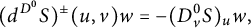 $$\begin{align*}(d^{D^0}S)^{\pm} (u,v)w = -(D^0_vS)_uw,\end{align*}$$
for all
 $(u,v,w)\in E_{\pm } \times E_{\mp }\times E_{\pm }$
.
$(u,v,w)\in E_{\pm } \times E_{\mp }\times E_{\pm }$
.
Proof The first formula is just (20). Since
 $D^0E_{\pm } \subset E_{\pm }$
and
$D^0E_{\pm } \subset E_{\pm }$
and
 $S_{E_{\pm }}E_{\mp }=0$
, we have
$S_{E_{\pm }}E_{\mp }=0$
, we have
 $$\begin{align*}(d^{D^0}S)^{\pm} (u,v)w = -D^0_{v}(S_{u})w -S_{{[}u,v{]}_H}w= -(D^0_{v}S)_{u}w -S_{D^0_vu}w -S_{{[}u,v{]}_H}w.\end{align*}$$
Using that
 $D^0$
is torsion-free, we can write
$D^0$
is torsion-free, we can write
 $[u,v]_H= D^0_uv-D^0_vu$
, since
$[u,v]_H= D^0_uv-D^0_vu$
, since
 $(D^0u)^*v=0$
for all
$(D^0u)^*v=0$
for all
 $(u,v)\in E_{\pm } \times E_{\mp }$
. Hence,
$(u,v)\in E_{\pm } \times E_{\mp }$
. Hence,
 $$\begin{align*}-S_{D^0_vu}w -S_{{[}u,v{]}_H}w= -S_{D^0_uv}w=0,\end{align*}$$
again because
 $D^0E_{\pm } \subset E_{\pm }$
and
$D^0E_{\pm } \subset E_{\pm }$
and
 $S_{E_{\pm }}E_{\mp }=0$
. This proves the lemma.
$S_{E_{\pm }}E_{\mp }=0$
. This proves the lemma.
Proposition 2.24 Let
 $ \delta $
be a divergence operator on
$ \delta $
be a divergence operator on
 $ E $
and
$ E $
and
 $ S\in \mathfrak {so}(E)^{\langle 1\rangle } $
such that the Levi-Civita generalized connection
$ S\in \mathfrak {so}(E)^{\langle 1\rangle } $
such that the Levi-Civita generalized connection
 $ D^0+S $
has divergence
$ D^0+S $
has divergence
 $ \delta $
. Then the Ricci curvatures
$ \delta $
. Then the Ricci curvatures
 $Ric^{\pm }_{\delta }$
of a generalized pseudo-Riemannian Lie group
$Ric^{\pm }_{\delta }$
of a generalized pseudo-Riemannian Lie group
 $(G,H,\mathcal G_g,\delta )$
with arbitrary divergence
$(G,H,\mathcal G_g,\delta )$
with arbitrary divergence
 $\delta \in E^*$
are related to the Ricci curvatures
$\delta \in E^*$
are related to the Ricci curvatures
 $Ric^{\pm }_0$
of
$Ric^{\pm }_0$
of
 $(G,H,\mathcal G_g,0)$
by
$(G,H,\mathcal G_g,0)$
by
 $$ \begin{align} Ric^{\pm}_{\delta} = Ric^{\pm}_0 + \operatorname{\mathrm{tr}}_{E_{\pm}}(d^{D^0}S)^{\pm} = Ric^{\pm}_0-D^0\delta|_{E_{\mp} \otimes E_{\pm}} ,\end{align} $$
where
 $$\begin{align*}(\operatorname{\mathrm{tr}}_{E_+}\alpha)(e_i,e_b) = \operatorname{\mathrm{tr}} (u\mapsto \alpha (u,e_i)e_b),\end{align*}$$
for any
 $\alpha \in E_+^*\otimes E_-^*\otimes E_+^*\otimes E_+$
and, similarly,
$\alpha \in E_+^*\otimes E_-^*\otimes E_+^*\otimes E_+$
and, similarly,
 $$\begin{align*}(\operatorname{\mathrm{tr}}_{E_-}\beta)(e_a,e_j) = \operatorname{\mathrm{tr}} (u\mapsto \beta(u,e_a)e_j),\end{align*}$$
when
 $\beta \in E_-^*\otimes E_+^*\otimes E_-^*\otimes E_-$
. Here, we are assuming the usual index ranges for
$\beta \in E_-^*\otimes E_+^*\otimes E_-^*\otimes E_-$
. Here, we are assuming the usual index ranges for
 $a,b$
and
$a,b$
and
 $i,j$
.
$i,j$
.
Proof An element
 $ S $
of the first generalized prolongation of
$ S $
of the first generalized prolongation of
 $\mathfrak {so}(E)$
such that
$\mathfrak {so}(E)$
such that
 $ D^0+S $
has divergence
$ D^0+S $
has divergence
 $ \delta $
exists due to Proposition 2.13. The first equation follows from Lemma 2.22 by taking traces. The formula
$ \delta $
exists due to Proposition 2.13. The first equation follows from Lemma 2.22 by taking traces. The formula
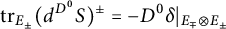 $$\begin{align*}\operatorname{\mathrm{tr}}_{E_{\pm}}(d^{D^0}S)^{\pm} = -D^0\delta|_{E_{\mp} \otimes E_{\pm}}\end{align*}$$
is a consequence of Lemma 2.23, since the trace maps
 $\operatorname {\mathrm{tr}}_{E_+}$
and
$\operatorname {\mathrm{tr}}_{E_+}$
and
 $\operatorname {\mathrm{tr}}_{E_-}$
are parallel for any metric generalized connection. In fact, for instance,
$\operatorname {\mathrm{tr}}_{E_-}$
are parallel for any metric generalized connection. In fact, for instance,
 $$\begin{align*}\operatorname{\mathrm{tr}}_{E_+}(d^{D^0}S)^+(e_i,e_b) = -\operatorname{\mathrm{tr}}_{E_+} \left((D^0_{e_i}S)e_b\right)= -D^0_{e_i}\left(\operatorname{\mathrm{tr}}_{E_+} S\right) e_b=-(D^0_{e_i}\delta) e_b,\end{align*}$$
where the
 $\operatorname {\mathrm{tr}}_{E_+} S\in E^*$
is defined by
$\operatorname {\mathrm{tr}}_{E_+} S\in E^*$
is defined by
![]() for all
for all
 $v\in E$
and we have used that
$v\in E$
and we have used that
 $\operatorname {\mathrm{tr}}_{E_+}(Sv)=\operatorname {\mathrm{tr}} (Sv)=\delta (v)$
for all
$\operatorname {\mathrm{tr}}_{E_+}(Sv)=\operatorname {\mathrm{tr}} (Sv)=\delta (v)$
for all
 $v\in E_+$
.
$v\in E_+$
.
Summarizing, we obtain the following theorem.
Theorem 2.25 The components
 $R_{ia}^{\delta }=Ric^+_{\delta } (e_i,e_a)$
and
$R_{ia}^{\delta }=Ric^+_{\delta } (e_i,e_a)$
and
 $R_{ai}^{\delta }=Ric^-_{\delta } (e_a,e_i)$
of the Ricci curvature tensors
$R_{ai}^{\delta }=Ric^-_{\delta } (e_a,e_i)$
of the Ricci curvature tensors
 $Ric^{\pm }_{\delta }$
of a generalized pseudo-Riemannian Lie group
$Ric^{\pm }_{\delta }$
of a generalized pseudo-Riemannian Lie group
 $(G,H,\mathcal G_g,\delta )$
with arbitrary divergence
$(G,H,\mathcal G_g,\delta )$
with arbitrary divergence
 $\delta \in E^*$
are given as follows:
$\delta \in E^*$
are given as follows:
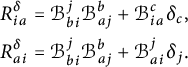 $$ \begin{align*} R_{ia}^{\delta}&= \mathcal{B}_{bi}^j \mathcal{B}_{aj}^b +\mathcal{B}_{ia}^c\delta_c,\\ R_{ai}^{\delta} &= \mathcal{B}_{bi}^j \mathcal{B}_{aj}^b + \mathcal{B}_{ai}^j\delta_j. \end{align*} $$
In particular, the Ricci tensor
 $Ric_{\delta } = Ric_{\delta }^+ \oplus Ric_{\delta }^-$
is symmetric if and only if,
$Ric_{\delta } = Ric_{\delta }^+ \oplus Ric_{\delta }^-$
is symmetric if and only if,
 $\delta $
satisfies the equation
$\delta $
satisfies the equation
 $\mathcal {B}_{ia}^c\delta _c = \mathcal {B}_{ai}^j\delta _j$
. It is skew-symmetric if
$\mathcal {B}_{ia}^c\delta _c = \mathcal {B}_{ai}^j\delta _j$
. It is skew-symmetric if
 $(G,H,\mathcal G_g,0)$
is generalized Einstein and
$(G,H,\mathcal G_g,0)$
is generalized Einstein and
 $\mathcal {B}_{ia}^c\delta _c = -\mathcal {B}_{ai}^j\delta _j$
. (Recall that we are always assuming the usual index ranges for
$\mathcal {B}_{ia}^c\delta _c = -\mathcal {B}_{ai}^j\delta _j$
. (Recall that we are always assuming the usual index ranges for
 $a, b$
and
$a, b$
and
 $i,j$
.)
$i,j$
.)
In terms of the linear maps
 $\Gamma _{u_{\pm }}: E_{\mp } \rightarrow E_{\pm }$
defined in (
18
) for
$\Gamma _{u_{\pm }}: E_{\mp } \rightarrow E_{\pm }$
defined in (
18
) for
 $u_{\pm } \in E_{\pm }$
, we have
$u_{\pm } \in E_{\pm }$
, we have
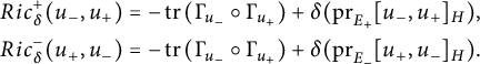 $$ \begin{align*} Ric_{\delta}^+ (u_-,u_+) &=-\operatorname{\mathrm{tr}} \left( \Gamma_{u_-}\circ \Gamma_{u_+}\right) + \delta (\mathrm{pr}_{E_+}[u_-,u_+]_H),\\ Ric_{\delta}^- (u_+,u_-) &= -\operatorname{\mathrm{tr}} \left( \Gamma_{u_-}\circ \Gamma_{u_+}\right) + \delta (\mathrm{pr}_{E_-}[u_+,u_-]_H). \end{align*} $$
The theorem shows that the Ricci curvature is completely determined by the one-form
 $\delta $
and the coefficients
$\delta $
and the coefficients
 $\mathcal {B}_{ajk}$
and
$\mathcal {B}_{ajk}$
and
 $\mathcal {B}_{ibc}$
of the Dorfman bracket in the orthonormal basis
$\mathcal {B}_{ibc}$
of the Dorfman bracket in the orthonormal basis
 $(e_A)=(e_a,e_i)$
. For future use, we do now compute the latter coefficients in terms of the coefficients of the Lie bracket (the structure constants) and the coefficients of the three-form H using (4). Recall that
$(e_A)=(e_a,e_i)$
. For future use, we do now compute the latter coefficients in terms of the coefficients of the Lie bracket (the structure constants) and the coefficients of the three-form H using (4). Recall that
 $(v_a)$
was a g-orthonormal basis of
$(v_a)$
was a g-orthonormal basis of
 $\mathfrak g$
. More precisely, we have
$\mathfrak g$
. More precisely, we have
 $g_{ab}=g(v_a,v_b) = \langle e_a,e_b\rangle = \eta _{ab}$
. We denote the corresponding structure constants of the Lie algebra
$g_{ab}=g(v_a,v_b) = \langle e_a,e_b\rangle = \eta _{ab}$
. We denote the corresponding structure constants of the Lie algebra
 $\mathfrak g$
by
$\mathfrak g$
by
 $\kappa _{ab}^c$
, such that
$\kappa _{ab}^c$
, such that
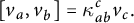 $$\begin{align*}[v_a,v_b]= \kappa_{ab}^cv_c.\end{align*}$$
Note that
 $\kappa _{abc} = \kappa _{ab}^dg_{dc}=\kappa _{ab}^d\eta _{dc}$
for
$\kappa _{abc} = \kappa _{ab}^dg_{dc}=\kappa _{ab}^d\eta _{dc}$
for
![]() .
.
Proposition 2.26 The Dorfman coefficients
 $\mathcal {B}_{ajk}$
,
$\mathcal {B}_{ajk}$
,
 $\mathcal {B}_{ibc}$
,
$\mathcal {B}_{ibc}$
,
 $\mathcal {B}_{abc}$
, and
$\mathcal {B}_{abc}$
, and
 $\mathcal {B}_{ijk}$
(
$\mathcal {B}_{ijk}$
(
 $a,b,c\in \{ 1,\ldots ,n\}$
,
$a,b,c\in \{ 1,\ldots ,n\}$
,
 $i,j,k\in \{ n+1,\ldots ,2n\}$
) are related to the structure constant
$i,j,k\in \{ n+1,\ldots ,2n\}$
) are related to the structure constant
 $\kappa _{abc}$
as follows:
$\kappa _{abc}$
as follows:
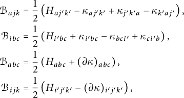 $$ \begin{align*} \mathcal{B}_{ajk} &= \frac12\left( H_{aj'k'}-\kappa_{aj'k'}+\kappa_{j'k'a}-\kappa_{k'aj'}\right),\\ \mathcal{B}_{ibc} &= \frac12\left( H_{i'bc}+\kappa_{i'bc}-\kappa_{bci'}+\kappa_{ci'b}\right),\\ \mathcal{B}_{abc} &= \frac12\left( H_{abc}+(\partial\kappa)_{abc}\right),\\ \mathcal{B}_{ijk} &= \frac12\left( H_{i'j'k'}-(\partial\kappa)_{i'j'k'} \right), \end{align*} $$
where
 $i'=i-n$
, for
$i'=i-n$
, for
 $i\in \{ n+1,\ldots , 2n\}$
and
$i\in \{ n+1,\ldots , 2n\}$
and
 $(\partial \kappa )_{abc}=\kappa _{abc}+\kappa _{bca}+\kappa _{cab}$
.
$(\partial \kappa )_{abc}=\kappa _{abc}+\kappa _{bca}+\kappa _{cab}$
.
Proof Using (4),we compute
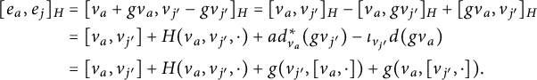 $$ \begin{align*} [e_a,e_j]_H &= [v_a+gv_a,v_{j'}-gv_{j'}]_H = [v_a,v_{j'}]_H -[v_a,gv_{j'}]_H+[gv_a,v_{j'}]_H\\ &= [v_a,v_{j'}] + H(v_a,v_{j'},\cdot ) +ad_{v_a}^*(gv_{j'}) -\iota_{v_{j'}}d(gv_a)\\ &=[v_a,v_{j'}] + H(v_a,v_{j'},\cdot ) +g(v_{j'},[v_a,\cdot ])+ g(v_a,[v_{j'}, \cdot ]). \end{align*} $$
It follows that
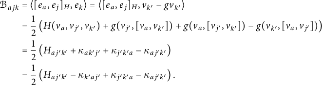 $$ \begin{align*} \mathcal{B}_{ajk} &= \langle [e_a,e_j]_H,e_k\rangle = \langle [e_a,e_j]_H,v_{k'}-gv_{k'}\rangle\\ &= \frac12 \left( H(v_a,v_{j'},v_{k'}) +g(v_{j'},[v_a,v_{k'} ])+ g(v_a,[v_{j'}, v_{k'} ])-g(v_{k'},[v_a,v_{j'}])\right)\\ &=\frac12 \left( H_{aj'k'} +\kappa_{ak'j'}+ \kappa_{j'k'a}-\kappa_{aj'k'}\right)\\ &=\frac12 \left( H_{aj'k'} -\kappa_{k'aj'}+ \kappa_{j'k'a}-\kappa_{aj'k'}\right). \end{align*} $$
The proof of the second formula is similar, where now
 $$\begin{align*}[e_i,e_b]_H = [v_{i'},v_b] + H(v_{i'},v_b,\cdot ) -g(v_b,[v_{i'},\cdot ]) -g(v_{i'},[v_b,\cdot ]).\end{align*}$$
The remaining equations are obtained in the same way.
The next result shows that the underlying metric g of an Einstein generalized pseudo-Riemannian Lie group can be freely rescaled without changing the Einstein property, provided that the three-form and the divergence are appropriately rescaled.
Proposition 2.27 Let g be a left-invariant pseudo-Riemannian metric and H a closed left-invariant three-form on a Lie group G. Consider
 $g'=\varepsilon \mu ^{-2}g$
and
$g'=\varepsilon \mu ^{-2}g$
and
 $H'=\varepsilon \mu ^{-2}H$
, where
$H'=\varepsilon \mu ^{-2}H$
, where
 $\varepsilon \in \{\pm 1\}$
and
$\varepsilon \in \{\pm 1\}$
and
 $\mu>0$
. Then the generalized pseudo-Riemannian Lie group
$\mu>0$
. Then the generalized pseudo-Riemannian Lie group
 $(G, H,\mathcal G_g)$
is Einstein with divergence
$(G, H,\mathcal G_g)$
is Einstein with divergence
 $\delta \in E^*$
if and only if
$\delta \in E^*$
if and only if
 $(G,H',\mathcal G_{g'})$
is Einstein with divergence
$(G,H',\mathcal G_{g'})$
is Einstein with divergence
 $\delta ' = \mu \delta $
.
$\delta ' = \mu \delta $
.
Proof Let
 $(v_a)$
be a g-orthonormal basis of
$(v_a)$
be a g-orthonormal basis of
 $\mathfrak {g}$
. Then
$\mathfrak {g}$
. Then
 $v_a' = \mu v_a$
defines a
$v_a' = \mu v_a$
defines a
 $g'$
-orthonormal basis
$g'$
-orthonormal basis
 $(v_a')$
. The corresponding basis
$(v_a')$
. The corresponding basis
 $(e_A')$
of E, where
$(e_A')$
of E, where
 $e_a'=v_a'+g'v_a'$
and
$e_a'=v_a'+g'v_a'$
and
 $e_i = v_i-g'v_i'$
, is still orthonormal with respect to the scalar product:
$e_i = v_i-g'v_i'$
, is still orthonormal with respect to the scalar product:
 $\langle e_A',e_B'\rangle = \varepsilon \langle e_A,e_B\rangle $
. The structure constants
$\langle e_A',e_B'\rangle = \varepsilon \langle e_A,e_B\rangle $
. The structure constants
![]() with respect to the basis
with respect to the basis
 $(v_a')$
are
$(v_a')$
are
 $\kappa _{abc}' = \varepsilon \mu \kappa _{abc}$
. Similarly,
$\kappa _{abc}' = \varepsilon \mu \kappa _{abc}$
. Similarly,
 $H'(v_a',v_b',v_c') = \varepsilon \mu H(v_a,v_b,v_c)$
. Finally, from these formulas and Proposition 2.26, we see that
$H'(v_a',v_b',v_c') = \varepsilon \mu H(v_a,v_b,v_c)$
. Finally, from these formulas and Proposition 2.26, we see that
![]() . Taking into account that
. Taking into account that
 $\langle e_A',e_B'\rangle = \varepsilon \langle e_A,e_B\rangle $
, we conclude that
$\langle e_A',e_B'\rangle = \varepsilon \langle e_A,e_B\rangle $
, we conclude that
![]() . Now Theorem 2.25 together with Proposition 2.15 shows that the coefficients of the Ricci curvatures
. Now Theorem 2.25 together with Proposition 2.15 shows that the coefficients of the Ricci curvatures
 $Ric$
of
$Ric$
of
 $(G, H,\mathcal G_g,\delta )$
and
$(G, H,\mathcal G_g,\delta )$
and
 $Ric'$
of
$Ric'$
of
 $(G,H',\mathcal G_{g'},\delta ')$
are related by
$(G,H',\mathcal G_{g'},\delta ')$
are related by
 $Ric'(e_A',e_B') = \mu ^2 Ric(e_A,e_B)$
.
$Ric'(e_A',e_B') = \mu ^2 Ric(e_A,e_B)$
.
Remark 2.28 Denote by
 $ \nabla $
the Levi-Civita connection of the pseudo-Riemannian metric
$ \nabla $
the Levi-Civita connection of the pseudo-Riemannian metric
 $ g $
and define its coefficients with respect to the orthonormal frame
$ g $
and define its coefficients with respect to the orthonormal frame
 $ (v_a) $
as
$ (v_a) $
as
![]() Then
Then
 $$\begin{align*}\Gamma_{abc}=\frac12\left(g([v_a,v_b],v_c)-g([v_b,v_c],v_a)+g([v_c,v_a],v_b) \right)=\frac12 (\kappa_{abc}-\kappa_{bca}+\kappa_{cab}) \end{align*}$$
and hence the Dorfman coefficients
 $\mathcal {B}_{ajk}$
and
$\mathcal {B}_{ajk}$
and
 $\mathcal {B}_{ibc}$
can be expressed by
$\mathcal {B}_{ibc}$
can be expressed by
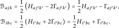 $$ \begin{align*} \mathcal{B}_{ajk}&=\frac12\left(H_{aj'k'}-2\Gamma_{aj'k'}\right)=\frac12H_{aj'k'}-\Gamma_{aj'k'},\\ \mathcal{B}_{ibc}&=\frac12\left(H_{i'bc}+2\Gamma_{i'bc}\right)=\frac12H_{i'bc}+\Gamma_{i'bc}. \end{align*} $$
Proposition 2.29 Let g be a left-invariant pseudo-Riemannian metric on a Lie group G. Consider the generalized pseudo-Riemannian Lie group
 $(G, H=0,\mathcal G_g)$
. Then the Ricci curvature
$(G, H=0,\mathcal G_g)$
. Then the Ricci curvature
 $Ric^+ _0={Ric^{\pm }_{\delta }|}_{\delta =0}$
of the generalized metric
$Ric^+ _0={Ric^{\pm }_{\delta }|}_{\delta =0}$
of the generalized metric
 $\mathcal G_g$
is related to the Ricci curvature
$\mathcal G_g$
is related to the Ricci curvature
 $Ric^g$
of the metric g by
$Ric^g$
of the metric g by
 $$\begin{align*}Ric^+_0(v-gv,u+gu) = Ric^-_0(u+gu,v-gv)=Ric^g(u,v) + (\nabla_u \tau)(v),\quad u,v\in \mathfrak{g}, \end{align*}$$
where
 $\tau \in \mathfrak {g}^*$
is the trace-form defined by
$\tau \in \mathfrak {g}^*$
is the trace-form defined by
 $\tau (v) = \operatorname {\mathrm {tr}} \mathrm {ad}_{v}$
.
$\tau (v) = \operatorname {\mathrm {tr}} \mathrm {ad}_{v}$
.
Proof The symmetry of the Ricci tensor of
 $\mathcal G_g$
follows from
$\mathcal G_g$
follows from
 $\delta =0$
. Therefore, it suffices to compute
$\delta =0$
. Therefore, it suffices to compute
 $R_{ia}=Ric^+(e_i,e_a)$
from Theorem 2.25 and to compare with
$R_{ia}=Ric^+(e_i,e_a)$
from Theorem 2.25 and to compare with
 $R^g_{ai'}=Ric^g(v_a,v_{i'})$
,
$R^g_{ai'}=Ric^g(v_a,v_{i'})$
,
 $i'=i-n$
. Note first that, by Remark 2.28, we have
$i'=i-n$
. Note first that, by Remark 2.28, we have
 $$\begin{align*}\mathcal{B}_{aj}^k = \Gamma_{aj'}^{k'},\quad \mathcal{B}_{ib}^c=\Gamma_{i'b}^c,\end{align*}$$
since
 $H=0$
and
$H=0$
and
 $\langle e_j,e_k\rangle = -\langle e_{j'},e_{k'}\rangle = -g(v_{j'},v_{k'})$
. Hence, using Lemma 2.9 and the fact that the Levi-Civita connection has zero torsion, we obtain
$\langle e_j,e_k\rangle = -\langle e_{j'},e_{k'}\rangle = -g(v_{j'},v_{k'})$
. Hence, using Lemma 2.9 and the fact that the Levi-Civita connection has zero torsion, we obtain
 $$\begin{align*}R_{ia} = \mathcal{B}_{bi}^j \mathcal{B}_{aj}^b= -\Gamma_{bi'}^{j'}\Gamma_{j'a}^b=-\Gamma_{bi'}^{j'}(\Gamma_{aj'}^b+ \kappa_{j'a}^b).\end{align*}$$
On the other hand, we have
 $$\begin{align*}R^g_{ai'}=\Gamma_{ai'}^d\Gamma_{fd}^f -\Gamma_{fi'}^d\Gamma_{ad}^f-\kappa_{fa}^d\Gamma_{di'}^f= \Gamma_{ai'}^d\Gamma_{fd}^f+R_{ia}.\end{align*}$$
To compute the first term, we note that since the Levi-Civita connection is metric, we have
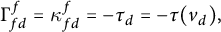 $$\begin{align*}\Gamma_{fd}^f = \kappa_{fd}^f = -\tau_d=-\tau (v_d),\end{align*}$$
and hence
 $$\begin{align*}\Gamma_{ai'}^d\Gamma_{fd}^f = -\Gamma_{ai'}^d\tau_d = (\nabla \tau)_{ai'}=(\nabla_{v_a}\tau)v_{i'}.\\[-35pt] \end{align*}$$
Corollary 2.30 Let g be a left-invariant pseudo-Riemannian metric on a Lie group G. Then the generalized pseudo-Riemannian Lie group
 $(G, H=0,\mathcal G_g)$
is Einstein with divergence
$(G, H=0,\mathcal G_g)$
is Einstein with divergence
 $\delta =0$
if and only if g satisfies the following Ricci soliton equation
$\delta =0$
if and only if g satisfies the following Ricci soliton equation
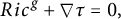 $$ \begin{align} Ric^g+\nabla \tau =0, \end{align} $$
where
 $\tau $
is the trace-form. The form
$\tau $
is the trace-form. The form
 $\tau $
is always closed and, hence, the solutions of the above equation are gradient Ricci solitons, if the first Betti number of the manifold G vanishes.
$\tau $
is always closed and, hence, the solutions of the above equation are gradient Ricci solitons, if the first Betti number of the manifold G vanishes.
Proof For all
 $u,v\in \mathfrak {g}$
, we have
$u,v\in \mathfrak {g}$
, we have
 $$\begin{align*}(d\tau )(u,v) = -\tau ([u,v]) = -\mathrm{tr}\, \mathrm{ad}_{[u,v]}= -\mathrm{tr}\, [\mathrm{ad}_u,\mathrm{ad}_v] =0.\\[-35pt] \end{align*}$$
Corollary 2.31 Let g be a left-invariant pseudo-Riemannian metric on a unimodular Lie group G. Then the generalized pseudo-Riemannian Lie group
 $(G, H=0,\mathcal G_g)$
is Einstein with divergence
$(G, H=0,\mathcal G_g)$
is Einstein with divergence
 $\delta =0$
if and only if g is Ricci-flat.
$\delta =0$
if and only if g is Ricci-flat.
3 Classification results in dimension 3
3.1 Preliminaries
Let G be a three-dimensional Lie group endowed with a left-invariant pseudo-Riemannian metric g and an orientation. We will identify g with a nondegenerate symmetric bilinear form
 $g\in \mathrm {Sym}^2\mathfrak {g}^*$
. We begin by showing that the Lie bracket can be encoded in an endomorphism L of
$g\in \mathrm {Sym}^2\mathfrak {g}^*$
. We begin by showing that the Lie bracket can be encoded in an endomorphism L of
 $\mathfrak {g}$
and study its properties.
$\mathfrak {g}$
and study its properties.
Following Milnor [Reference MilnorM], but allowing indefinite metrics, we denote by
 $L\in \mathrm {End}\, \mathfrak {g}$
the endomorphism such that
$L\in \mathrm {End}\, \mathfrak {g}$
the endomorphism such that
 $$ \begin{align} [u,v] = L(u\times v),\quad \forall u,v\in \mathfrak{g},\end{align} $$
where the cross-product
 $\times \in \bigwedge ^2\mathfrak {g}^*\otimes \mathfrak {g}$
is defined by
$\times \in \bigwedge ^2\mathfrak {g}^*\otimes \mathfrak {g}$
is defined by
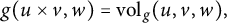 $$ \begin{align} g(u\times v,w) = \mathrm{vol}_g(u,v,w),\end{align} $$
using the metric volume form
 $\mathrm {vol}_g$
. In terms of an oriented orthonormal basis
$\mathrm {vol}_g$
. In terms of an oriented orthonormal basis
 $(v_a)$
, we have
$(v_a)$
, we have
 $$\begin{align*}v_a\times v_b = \varepsilon_c v_c,\quad \varepsilon_c=g(v_c,v_c),\end{align*}$$
for every cyclic permutation
 $(a,b,c)$
of
$(a,b,c)$
of
 $\{ 1,2,3\}$
. This implies that
$\{ 1,2,3\}$
. This implies that
 $$ \begin{align} [v_a,v_b] = \varepsilon_c Lv_c,\quad\forall\quad\mbox{cyclic}\quad (a,b,c)\in \mathfrak{S}_3.\end{align} $$
We denote by
 $(L^a_{\phantom {a}b})$
the matrix of L in the above basis,
$(L^a_{\phantom {a}b})$
the matrix of L in the above basis,
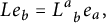 $$\begin{align*}Le_b= L^a_{\phantom{a}b}e_a,\end{align*}$$
and by
 $L^{ab}=L^a_{\phantom {a}c}g^{cb}$
, the coefficients of the corresponding tensor
$L^{ab}=L^a_{\phantom {a}c}g^{cb}$
, the coefficients of the corresponding tensor
 $L \circ g^{-1} \in \mathrm {Hom}(\mathfrak {g}^*,\mathfrak {g}) \cong \mathfrak {g}\otimes \mathfrak {g}$
.
$L \circ g^{-1} \in \mathrm {Hom}(\mathfrak {g}^*,\mathfrak {g}) \cong \mathfrak {g}\otimes \mathfrak {g}$
.
From (25), we see that the structure constants
 $\kappa _{ab}^c$
of
$\kappa _{ab}^c$
of
 $\mathfrak {g}$
with respect to the basis
$\mathfrak {g}$
with respect to the basis
 $(v_a)$
can be written as
$(v_a)$
can be written as
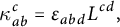 $$\begin{align*}\kappa_{ab}^c = \varepsilon_{abd}L^{cd},\end{align*}$$
where
 $\varepsilon _{abd}=\mathrm {vol}_g(v_a,v_b,v_d)$
(in particular,
$\varepsilon _{abd}=\mathrm {vol}_g(v_a,v_b,v_d)$
(in particular,
 $\varepsilon _{123}=1$
).
$\varepsilon _{123}=1$
).
The following lemma is a straightforward generalization of [Reference MilnorM, Lemma 4.1].
Lemma 3.1 The endomorphism L is symmetric with respect to g if and only if
 $\mathfrak {g}$
is unimodular.
$\mathfrak {g}$
is unimodular.
Proof Note first that L is symmetric with respect to g if and only if the matrix
 $(L^{ab})$
is symmetric. Therefore, the calculation
$(L^{ab})$
is symmetric. Therefore, the calculation
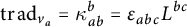 $$\begin{align*}\operatorname{\mathrm{tr}} \mathrm{ad}_{v_a} = \kappa_{ab}^b = \varepsilon_{abc}L^{bc}\end{align*}$$
shows that L is symmetric if and only if
 $\operatorname {\mathrm{tr}} \mathrm {ad}_{v_a}=0$
for all a, i.e., if and only if
$\operatorname {\mathrm{tr}} \mathrm {ad}_{v_a}=0$
for all a, i.e., if and only if
 $\mathfrak g$
is unimodular.
$\mathfrak g$
is unimodular.
Proposition 3.2 Let g be a nondegenerate symmetric bilinear form on an oriented three-dimensional unimodular Lie algebra
 $ \mathfrak {g} $
. Then there exists an orthonormal basis
$ \mathfrak {g} $
. Then there exists an orthonormal basis
 $(v_a)$
of
$(v_a)$
of
 $(\mathfrak {g},g)$
such that
$(\mathfrak {g},g)$
such that
 $g(v_1,v_1)=g(v_2,v_2)$
and such that the symmetric endomorphism L defined in Equation (23) is represented by one of the following matrices:
$g(v_1,v_1)=g(v_2,v_2)$
and such that the symmetric endomorphism L defined in Equation (23) is represented by one of the following matrices:
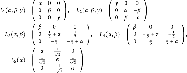 $$ \begin{align*}L_1(\alpha , \beta, \gamma ) &= \left( \begin{array}{ccc}\alpha &0&0\\ 0&\beta& 0\\ 0&0&\gamma \end{array}\right),\quad L_2(\alpha , \beta,\gamma )=\left( \begin{array}{ccc} \gamma &0&0\\ 0&\alpha &-\beta\\ 0&\beta&\alpha \end{array}\right),\\ L_3(\alpha , \beta)&=\left( \begin{array}{ccc}\beta&0&0\\0&\frac12+\alpha &\frac12\\ 0&-\frac12&-\frac12 +\alpha\\ \end{array}\right),\quad L_4(\alpha , \beta)= \left( \begin{array}{ccc} \beta&0&0\\0&-\frac12+\alpha &-\frac12\\ 0&\frac12&\frac12 +\alpha\\ \end{array}\right),\\ L_5(\alpha) &=\left( \begin{array}{ccc}\alpha&\frac{1}{\sqrt{2}}&0\\ \frac{1}{\sqrt{2}}&\alpha& \frac{1}{\sqrt{2}}\\ 0&-\frac{1}{\sqrt{2}}&\alpha\end{array}\right), \end{align*} $$
where
 $\alpha , \beta ,\gamma \in \mathbb {R}$
and
$\alpha , \beta ,\gamma \in \mathbb {R}$
and
 $g(v_3,v_3)=-g(v_2,v_2)$
for the normal forms
$g(v_3,v_3)=-g(v_2,v_2)$
for the normal forms
 $L_2,\ldots , L_5$
. If g is definite, then the orthonormal basis can be chosen such that L is represented by a diagonal matrix
$L_2,\ldots , L_5$
. If g is definite, then the orthonormal basis can be chosen such that L is represented by a diagonal matrix
 $L_1(\alpha , \beta , \gamma )$
and each diagonal matrix is realized in this way. If g is indefinite, then each of the above normal forms is realized by some unimodular Lie bracket.
$L_1(\alpha , \beta , \gamma )$
and each diagonal matrix is realized in this way. If g is indefinite, then each of the above normal forms is realized by some unimodular Lie bracket.
Proof It is well known that every symmetric endomorphism on a Euclidean vector space can be diagonalized. According to [Reference Cortés, Ehlert, Haupt and LindemannCEHL, Lemma 2.2] and the references therein, for an indefinite scalar product on a three-dimensional vector space, there are the five normal forms of a symmetric bilinear form, from which one easily obtains the five normal forms
 $L_1(\alpha , \beta , \gamma ), L_2(\alpha , \beta , \gamma ), L_3(\alpha , \beta ), L_4(\alpha , \beta )$
, and
$L_1(\alpha , \beta , \gamma ), L_2(\alpha , \beta , \gamma ), L_3(\alpha , \beta ), L_4(\alpha , \beta )$
, and
 $L_5(\alpha )$
for a symmetric endomorphism. It remains to check that for each of these normal forms
$L_5(\alpha )$
for a symmetric endomorphism. It remains to check that for each of these normal forms
 $(L^a_{\phantom {a}b})$
, the bracket with structure constants
$(L^a_{\phantom {a}b})$
, the bracket with structure constants
 $\kappa _{ab}^c = \varepsilon _{abd}L^{cd}$
satisfies the Jacobi identity.
$\kappa _{ab}^c = \varepsilon _{abd}L^{cd}$
satisfies the Jacobi identity.
All the cases can be treated simultaneously by considering
 $(L^a_{\phantom {a}b})$
of the form
$(L^a_{\phantom {a}b})$
of the form
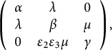 $$\begin{align*}\left(\begin{array}{ccc}\alpha &\lambda &0\\ \lambda &\beta &\mu \\ 0&\varepsilon_2\varepsilon_3\mu&\gamma\end{array} \right), \\[-9pt]\end{align*}$$
where
 $\lambda ,\mu \in \mathbb {R}$
. For the corresponding endomorphism L, we have
$\lambda ,\mu \in \mathbb {R}$
. For the corresponding endomorphism L, we have

where we have used that
 $\varepsilon _1=\varepsilon _2$
.
$\varepsilon _1=\varepsilon _2$
.
3.2 Classification in the case of zero divergence
3.2.1 Unimodular Lie groups
Proposition 3.3 If
 $(H,\mathcal G_g,\delta =0)$
is a divergence-free generalized Einstein structure on an oriented three-dimensional unimodular Lie group G, then there exists a
$(H,\mathcal G_g,\delta =0)$
is a divergence-free generalized Einstein structure on an oriented three-dimensional unimodular Lie group G, then there exists a
 $ g $
-orthonormal basis
$ g $
-orthonormal basis
 $(v_a)$
of
$(v_a)$
of
 $\mathfrak g$
such that
$\mathfrak g$
such that
 $g(v_1,v_1)=g(v_2,v_2)$
and such that the symmetric endomorphism L defined in equation (
23
) is either of the form
$g(v_1,v_1)=g(v_2,v_2)$
and such that the symmetric endomorphism L defined in equation (
23
) is either of the form
 $ L_1(\alpha ,\beta ,\gamma ) $
, that is
$ L_1(\alpha ,\beta ,\gamma ) $
, that is
 $ L $
is diagonalizable by an orthonormal basis, or of one of the forms
$ L $
is diagonalizable by an orthonormal basis, or of one of the forms
 $ L_3(0,0) $
or
$ L_3(0,0) $
or
 $ L_4(0,0) $
. In the nondiagonalizable case, the three-form
$ L_4(0,0) $
. In the nondiagonalizable case, the three-form
 $ H $
is zero.
$ H $
is zero.
Proof In the Euclidean case, any symmetric endomorphism is always diagonalizable by an orthonormal basis. So we may assume that the scalar product is indefinite. By Proposition 3.2, there is an orthonormal basis
 $ (v_a) $
, such that the endomorphism
$ (v_a) $
, such that the endomorphism
 $ L $
takes one of the normal forms
$ L $
takes one of the normal forms
 $L_1(\alpha , \beta , \gamma ), L_2(\alpha , \beta , \gamma ), L_3(\alpha , \beta ), L_4(\alpha , \beta )$
, or
$L_1(\alpha , \beta , \gamma ), L_2(\alpha , \beta , \gamma ), L_3(\alpha , \beta ), L_4(\alpha , \beta )$
, or
 $L_5(\alpha )$
from said proposition. As in the proof of Proposition 3.2, we can treat all cases at once by considering the matrix
$L_5(\alpha )$
from said proposition. As in the proof of Proposition 3.2, we can treat all cases at once by considering the matrix
 $$\begin{align*}\left(\begin{array}{ccc}\alpha &\lambda &0\\ \lambda &\beta &\mu \\ 0&-\mu&\gamma\end{array} \right). \end{align*}$$
Recall that we assume
 $ \varepsilon _{1}=\varepsilon _2=-\varepsilon _{3} $
, where
$ \varepsilon _{1}=\varepsilon _2=-\varepsilon _{3} $
, where
 $ \varepsilon _a=g(v_a,v_a) $
. Using equation (25), we obtain the structure constants
$ \varepsilon _a=g(v_a,v_a) $
. Using equation (25), we obtain the structure constants
 $ \kappa _{abc}=\varepsilon _c\kappa _{ab}^c $
of the Lie algebra in the following way. The bracket is given by
$ \kappa _{abc}=\varepsilon _c\kappa _{ab}^c $
of the Lie algebra in the following way. The bracket is given by
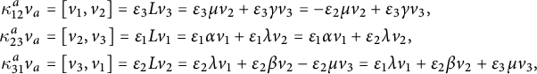 $$\begin{align*}\begin{aligned} \kappa_{12}^av_a&=[v_1,v_2]=\varepsilon_{3}Lv_3=\varepsilon_3\mu v_2+\varepsilon_3\gamma v_3=-\varepsilon_2\mu v_2+\varepsilon_3\gamma v_3,\\ \kappa_{23}^av_a&=[v_2,v_3]=\varepsilon_{1}Lv_1=\varepsilon_{1}\alpha v_1+\varepsilon_{1}\lambda v_2=\varepsilon_{1}\alpha v_1+\varepsilon_{2}\lambda v_2,\\ \kappa_{31}^av_a&=[v_3,v_1]=\varepsilon_{2}Lv_2=\varepsilon_{2}\lambda v_1+\varepsilon_{2}\beta v_2-\varepsilon_{2}\mu v_3=\varepsilon_{1}\lambda v_1+\varepsilon_{2}\beta v_2+\varepsilon_{3}\mu v_3, \end{aligned}\end{align*}$$
and hence
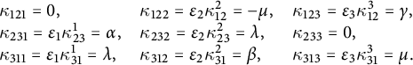 $$\begin{align*}\begin{array}{lll} \kappa_{121}=0,&\kappa_{122}=\varepsilon_{2}\kappa_{12}^2=-\mu,&\kappa_{123}=\varepsilon_{3}\kappa_{12}^3=\gamma,\\ \kappa_{231}=\varepsilon_{1}\kappa_{23}^1=\alpha,&\kappa_{232}=\varepsilon_{2}\kappa_{23}^2=\lambda,&\kappa_{233}=0,\\ \kappa_{311}=\varepsilon_{1}\kappa_{31}^1=\lambda,&\kappa_{312}=\varepsilon_{2}\kappa_{31}^2=\beta,&\kappa_{313}=\varepsilon_{3}\kappa_{31}^3=\mu.\end{array} \end{align*}$$
The remaining structure constants are determined by the skew-symmetry of
 $ \kappa _{abc} $
in the first two components.
$ \kappa _{abc} $
in the first two components.
By Proposition 2.26, the Dorfman coefficients are given as follows:
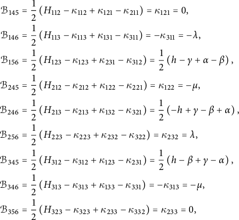 $$ \begin{align*} \mathcal{B}_{145}&=\frac12\left(H_{112}-\kappa_{112}+\kappa_{121}-\kappa_{211}\right)=\kappa_{121}=0,\\ \mathcal{B}_{146}&=\frac12\left(H_{113}-\kappa_{113}+\kappa_{131}-\kappa_{311}\right)=-\kappa_{311}=-\lambda,\\ \mathcal{B}_{156}&=\frac12\left(H_{123}-\kappa_{123}+\kappa_{231}-\kappa_{312}\right)=\frac12\left(h-\gamma+\alpha-\beta\right),\\ \mathcal{B}_{245}&=\frac12\left(H_{212}-\kappa_{212}+\kappa_{122}-\kappa_{221}\right)=\kappa_{122}=-\mu,\\ \mathcal{B}_{246}&=\frac12\left(H_{213}-\kappa_{213}+\kappa_{132}-\kappa_{321}\right)=\frac12\left(-h+\gamma-\beta+\alpha\right),\\ \mathcal{B}_{256}&=\frac12\left(H_{223}-\kappa_{223}+\kappa_{232}-\kappa_{322}\right)=\kappa_{232}=\lambda,\\ \mathcal{B}_{345}&=\frac12\left(H_{312}-\kappa_{312}+\kappa_{123}-\kappa_{231}\right)=\frac12\left(h-\beta+\gamma-\alpha\right),\\ \mathcal{B}_{346}&=\frac12\left(H_{313}-\kappa_{313}+\kappa_{133}-\kappa_{331}\right)=-\kappa_{313}=-\mu,\\ \mathcal{B}_{356}&=\frac12\left(H_{323}-\kappa_{323}+\kappa_{233}-\kappa_{332}\right)=\kappa_{233}=0, \end{align*} $$
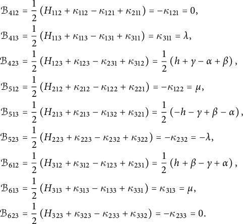 $$ \begin{align*} \mathcal{B}_{412}&=\frac12\left(H_{112}+\kappa_{112}-\kappa_{121}+\kappa_{211}\right)=-\kappa_{121}=0,\\ \mathcal{B}_{413}&=\frac12\left(H_{113}+\kappa_{113}-\kappa_{131}+\kappa_{311}\right)=\kappa_{311}=\lambda,\\ \mathcal{B}_{423}&=\frac12\left(H_{123}+\kappa_{123}-\kappa_{231}+\kappa_{312}\right)=\frac12\left(h+\gamma-\alpha+\beta\right),\\ \mathcal{B}_{512}&=\frac12\left(H_{212}+\kappa_{212}-\kappa_{122}+\kappa_{221}\right)=-\kappa_{122}=\mu,\\ \mathcal{B}_{513}&=\frac12\left(H_{213}+\kappa_{213}-\kappa_{132}+\kappa_{321}\right)=\frac12\left(-h-\gamma+\beta-\alpha\right),\\ \mathcal{B}_{523}&=\frac12\left(H_{223}+\kappa_{223}-\kappa_{232}+\kappa_{322}\right)=-\kappa_{232}=-\lambda,\\ \mathcal{B}_{612}&=\frac12\left(H_{312}+\kappa_{312}-\kappa_{123}+\kappa_{231}\right)=\frac12\left(h+\beta-\gamma+\alpha\right),\\ \mathcal{B}_{613}&=\frac12\left(H_{313}+\kappa_{313}-\kappa_{133}+\kappa_{331}\right)=\kappa_{313}=\mu,\\ \mathcal{B}_{623}&=\frac12\left(H_{323}+\kappa_{323}-\kappa_{233}+\kappa_{332}\right)=-\kappa_{233}=0.\\[-15pt] \end{align*} $$
Now, Theorem 2.25 allows us to compute the Ricci curvature (for zero divergence
 $\delta $
) with respect to the orthonormal basis
$\delta $
) with respect to the orthonormal basis
 $(e_A)=(e_a,e_i)$
,
$(e_A)=(e_a,e_i)$
,
 $e_a = v_a + gv_a$
,
$e_a = v_a + gv_a$
,
 $e_i=v_{i'}-gv_{i'}$
, of
$e_i=v_{i'}-gv_{i'}$
, of
 $E=\mathfrak g \oplus \mathfrak g^*$
as
$E=\mathfrak g \oplus \mathfrak g^*$
as
 $$ \begin{align} R_{ia} = \sum_{j,b}\mathcal{B}_{bi}^j \mathcal{B}_{aj}^b = \sum_{j,b} \mathcal{B}_{bij} \mathcal{B}_{ajb}(-\varepsilon_{j'})\varepsilon_b = \sum_{j,b} \mathcal{B}_{bij} \mathcal{B}_{jab}\varepsilon_{j'}\varepsilon_b,\\[-15pt]\nonumber \end{align} $$
where we have used that
 $\langle e_i,e_i\rangle = -\langle e_{i'},e_{i'}\rangle = -\varepsilon _{i'}$
and the standard index ranges
$\langle e_i,e_i\rangle = -\langle e_{i'},e_{i'}\rangle = -\varepsilon _{i'}$
and the standard index ranges
 $a,b\in \{ 1,2,3\}$
,
$a,b\in \{ 1,2,3\}$
,
 $i,j\in \{ 4,5,6\}$
.
$i,j\in \{ 4,5,6\}$
.
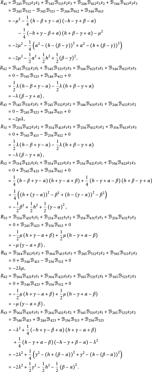 $$ \begin{align*} R_{41}&=\mathcal{B}_{245}\mathcal{B}_{512}\varepsilon_{2}\varepsilon_2+\mathcal{B}_{345}\mathcal{B}_{513}\varepsilon_{2}\varepsilon_3+\mathcal{B}_{246}\mathcal{B}_{612}\varepsilon_{3}\varepsilon_2+\mathcal{B}_{346}\mathcal{B}_{613}\varepsilon_{3}\varepsilon_3\\ &=\mathcal{B}_{245}\mathcal{B}_{512}-\mathcal{B}_{345}\mathcal{B}_{513}-\mathcal{B}_{246}\mathcal{B}_{612}+\mathcal{B}_{346}\mathcal{B}_{613}\\ &=-\mu^2-\frac14\left(h-\beta+\gamma-\alpha\right)\left(-h-\gamma+\beta-\alpha\right)\\ &\qquad-\frac14\left(-h+\gamma-\beta+\alpha\right)\left(h+\beta-\gamma+\alpha\right)-\mu^2\\ &=-2\mu^2-\frac14\left(\alpha^2-\left(h-\left(\beta-\gamma\right)\right)^2+\alpha^2-\left(h+\left(\beta-\gamma\right)\right)^2\right)\\ &=-2\mu^2-\frac12\alpha^2+\frac12h^2+\frac12(\beta-\gamma)^2,\\ R_{42}&=\mathcal{B}_{145}\mathcal{B}_{521}\varepsilon_{2}\varepsilon_1+\mathcal{B}_{345}\mathcal{B}_{523}\varepsilon_{2}\varepsilon_3+\mathcal{B}_{146}\mathcal{B}_{621}\varepsilon_{3}\varepsilon_1+\mathcal{B}_{346}\mathcal{B}_{623}\varepsilon_{3}\varepsilon_3\\ &=0-\mathcal{B}_{345}\mathcal{B}_{523}+\mathcal{B}_{146}\mathcal{B}_{612}+0\\ &=\frac12\lambda\left(h-\beta+\gamma-\alpha\right)-\frac12\lambda\left(h+\beta-\gamma+\alpha\right)\\ &=-\lambda\left(\beta-\gamma+\alpha\right),\\ R_{43}&=\mathcal{B}_{145}\mathcal{B}_{531}\varepsilon_{2}\varepsilon_1+\mathcal{B}_{245}\mathcal{B}_{532}\varepsilon_{2}\varepsilon_2+\mathcal{B}_{146}\mathcal{B}_{631}\varepsilon_{3}\varepsilon_1+\mathcal{B}_{246}\mathcal{B}_{632}\varepsilon_{3}\varepsilon_2\\ &=0-\mathcal{B}_{245}\mathcal{B}_{523}+\mathcal{B}_{146}\mathcal{B}_{613}+0\\ &=-2\mu\lambda,\\ R_{51}&=\mathcal{B}_{254}\mathcal{B}_{412}\varepsilon_{1}\varepsilon_2+\mathcal{B}_{354}\mathcal{B}_{413}\varepsilon_{1}\varepsilon_3+\mathcal{B}_{256}\mathcal{B}_{612}\varepsilon_{3}\varepsilon_2+\mathcal{B}_{356}\mathcal{B}_{613}\varepsilon_{3}\varepsilon_3\\ &=0+\mathcal{B}_{345}\mathcal{B}_{413}-\mathcal{B}_{256}\mathcal{B}_{612}+0\\ &=\frac12\lambda\left(h-\beta+\gamma-\alpha\right)-\frac12\lambda\left(h+\beta-\gamma+\alpha\right)\\ &=-\lambda\left(\beta-\gamma+\alpha\right),\\ R_{52}&=\mathcal{B}_{154}\mathcal{B}_{421}\varepsilon_{1}\varepsilon_1+\mathcal{B}_{354}\mathcal{B}_{423}\varepsilon_{1}\varepsilon_3+\mathcal{B}_{156}\mathcal{B}_{621}\varepsilon_{3}\varepsilon_1+\mathcal{B}_{356}\mathcal{B}_{623}\varepsilon_{3}\varepsilon_3\\ &=0+\mathcal{B}_{345}\mathcal{B}_{423}+\mathcal{B}_{156}\mathcal{B}_{612}+0\\ &=\frac14\left(h-\beta+\gamma-\alpha\right)\left(h+\gamma-\alpha+\beta\right)+\frac14\left(h-\gamma+\alpha-\beta\right)\left(h+\beta-\gamma+\alpha\right)\\ &=\frac14\left(\left(h+\left(\gamma-\alpha\right)\right)^2-\beta^2+\left(h-\left(\gamma-\alpha\right)\right)^2-\beta^2\right)\\ &=-\frac12\beta^2+\frac12h^2+\frac12\left(\gamma-\alpha\right)^2,\\ R_{53}&=\mathcal{B}_{154}\mathcal{B}_{431}\varepsilon_{1}\varepsilon_1+\mathcal{B}_{254}\mathcal{B}_{432}\varepsilon_{1}\varepsilon_2+\mathcal{B}_{156}\mathcal{B}_{631}\varepsilon_{3}\varepsilon_1+\mathcal{B}_{256}\mathcal{B}_{632}\varepsilon_{3}\varepsilon_2\\ &=0+\mathcal{B}_{245}\mathcal{B}_{423}+\mathcal{B}_{156}\mathcal{B}_{613}+0\\ &=-\frac12\mu\left(h+\gamma-\alpha+\beta\right)+\frac12\mu\left(h-\gamma+\alpha-\beta\right)\\ &=-\mu\left(\gamma-\alpha+\beta\right),\\ R_{61}&=\mathcal{B}_{264}\mathcal{B}_{412}\varepsilon_{1}\varepsilon_2+\mathcal{B}_{364}\mathcal{B}_{413}\varepsilon_{1}\varepsilon_3+\mathcal{B}_{265}\mathcal{B}_{512}\varepsilon_{2}\varepsilon_2+\mathcal{B}_{365}\mathcal{B}_{513}\varepsilon_{2}\varepsilon_3\\ &=0+\mathcal{B}_{346}\mathcal{B}_{413}-\mathcal{B}_{256}\mathcal{B}_{512}+0\\ &=-2\lambda\mu,\\ R_{62}&=\mathcal{B}_{164}\mathcal{B}_{421}\varepsilon_{1}\varepsilon_1+\mathcal{B}_{364}\mathcal{B}_{423}\varepsilon_{1}\varepsilon_3+\mathcal{B}_{165}\mathcal{B}_{521}\varepsilon_{2}\varepsilon_1+\mathcal{B}_{365}\mathcal{B}_{523}\varepsilon_{2}\varepsilon_3\\ &=0+\mathcal{B}_{346}\mathcal{B}_{423}+\mathcal{B}_{156}\mathcal{B}_{512}+0\\ &=-\frac12\mu\left(h+\gamma-\alpha+\beta\right)+\frac12\mu\left(h-\gamma+\alpha-\beta\right)\\ &=-\mu\left(\gamma-\alpha+\beta\right),\\ R_{63}&=\mathcal{B}_{164}\mathcal{B}_{431}\varepsilon_{1}\varepsilon_1+\mathcal{B}_{264}\mathcal{B}_{432}\varepsilon_{1}\varepsilon_2+\mathcal{B}_{165}\mathcal{B}_{531}\varepsilon_{2}\varepsilon_1+\mathcal{B}_{265}\mathcal{B}_{532}\varepsilon_{2}\varepsilon_2\\ &=\mathcal{B}_{146}\mathcal{B}_{413}+\mathcal{B}_{246}\mathcal{B}_{423}+\mathcal{B}_{156}\mathcal{B}_{513}+\mathcal{B}_{256}\mathcal{B}_{523}\\ &=-\lambda^2+\frac14\left(-h+\gamma-\beta+\alpha\right)\left(h+\gamma-\alpha+\beta\right)\\ &\quad+\frac14\left(h-\gamma+\alpha-\beta\right)\left(-h-\gamma+\beta-\alpha\right)-\lambda^2\\ &=-2\lambda^2+\frac14\left(\gamma^2-\left(h+\left(\beta-\alpha\right)\right)^2+\gamma^2-\left(h-\left(\beta-\alpha\right)\right)^2\right)\\ &=-2\lambda^2+\frac12\gamma^2-\frac12h^2-\frac12\left(\beta-\alpha\right)^2. \end{align*} $$
We see that the Einstein equations yield a system of homogeneous quadratic equations in the real variables
 $ \alpha ,\beta ,\gamma ,\lambda , $
and
$ \alpha ,\beta ,\gamma ,\lambda , $
and
 $ \mu $
.
$ \mu $
.
The normal form
 $ L_5(\alpha ) $
is excluded by equation
$ L_5(\alpha ) $
is excluded by equation
 $ R_{43}=0 $
for any
$ R_{43}=0 $
for any
 $ \alpha \in \mathbb {R} $
.
$ \alpha \in \mathbb {R} $
.
Equation
 $ R_{53}=0 $
for the normal form
$ R_{53}=0 $
for the normal form
 $ L_2(\alpha ,\beta ,\gamma ) $
reads as
$ L_2(\alpha ,\beta ,\gamma ) $
reads as
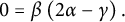 $$\begin{align*}0=\beta\left(2\alpha-\gamma\right). \end{align*}$$
If
 $ \beta =0 $
, then the matrix is diagonal, so assume that
$ \beta =0 $
, then the matrix is diagonal, so assume that
 $ \gamma =2\alpha $
. Then
$ \gamma =2\alpha $
. Then
 $ R_{52}=0 $
yields
$ R_{52}=0 $
yields
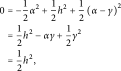 $$ \begin{align*} 0&=-\frac12\alpha^2+\frac12h^2+\frac12\left(\alpha-\gamma\right)^2\\ &=\frac12h^2-\alpha\gamma+\frac12\gamma^2\\ &=\frac12h^2, \end{align*} $$
and hence
 $ h=0 $
. Therefore, equation
$ h=0 $
. Therefore, equation
 $ R_{41}=0 $
is
$ R_{41}=0 $
is
 $$ \begin{align*} 0=-2\beta^2-\frac12\gamma^2, \end{align*} $$
which gives
 $ \beta =\gamma =0 $
. Hence,
$ \beta =\gamma =0 $
. Hence,
 $ L $
is diagonalizable by an orthonormal basis.
$ L $
is diagonalizable by an orthonormal basis.
If we consider the normal form
 $ L_3(\alpha ,\beta ) $
, the equation
$ L_3(\alpha ,\beta ) $
, the equation
 $ R_{53}=0 $
is
$ R_{53}=0 $
is
 $$ \begin{align*} 0=-\frac12\left(\alpha-\frac12-\beta+\alpha+\frac12\right)=-\frac12\left(2\alpha-\beta\right), \end{align*} $$
and hence
 $ 2\alpha =\beta $
. Now, the equation for
$ 2\alpha =\beta $
. Now, the equation for
 $ R_{41} $
yields
$ R_{41} $
yields
 $$ \begin{align*} 0&=-2\left(\frac12\right)^2-\frac12\beta^2+\frac12h^2+\frac12\left(\alpha+\frac12-\alpha+\frac12\right)^2\\ &=-\frac12-\frac12\beta^2+\frac12h^2+\frac12\\ &=-\frac12\beta^2+\frac12h^2, \end{align*} $$
and hence
 $ \beta ^2=h^2 $
. Applying this to the equation
$ \beta ^2=h^2 $
. Applying this to the equation
 $ R_{52}=0 $
gives
$ R_{52}=0 $
gives
 $$ \begin{align*} 0&=-\frac12\left(\frac12+\alpha\right)^2+\frac12h^2+\frac12\left(\alpha-\frac12-\beta\right)^2\\ &=-\frac12\left(\frac12+\alpha\right)^2+\frac12h^2+\frac12\left(-\alpha-\frac12\right)^2\\ &=\frac12h^2. \end{align*} $$
From that, see
 $ h=0 $
, and therefore
$ h=0 $
, and therefore
 $ \alpha =\beta =0 $
.
$ \alpha =\beta =0 $
.
A similar computation for
 $ L_4(\alpha ,\beta ) $
shows that the only possibility is
$ L_4(\alpha ,\beta ) $
shows that the only possibility is
 $ L_4(0,0) $
with
$ L_4(0,0) $
with
 $ h=0 $
.
$ h=0 $
.
Theorem 3.4 Let
 $(H,\mathcal {G}_g)$
be a divergence-free generalized Einstein structure on an oriented three-dimensional unimodular Lie group G. If the endomorphism
$(H,\mathcal {G}_g)$
be a divergence-free generalized Einstein structure on an oriented three-dimensional unimodular Lie group G. If the endomorphism
 $L\in \mathrm {End}\, \mathfrak g$
defined in (
24
) is diagonalizable, then there exists an oriented g-orthonormal basis
$L\in \mathrm {End}\, \mathfrak g$
defined in (
24
) is diagonalizable, then there exists an oriented g-orthonormal basis
 $(v_a)$
of
$(v_a)$
of
 $\mathfrak g = \mathrm {Lie}\, G$
and
$\mathfrak g = \mathrm {Lie}\, G$
and
 $\alpha _1,\alpha _2,\alpha _3, h \in \mathbb {R}$
such that
$\alpha _1,\alpha _2,\alpha _3, h \in \mathbb {R}$
such that
 $$ \begin{align} [v_a,v_b] = \alpha_c \varepsilon_cv_c,\quad \forall\quad\mbox{cyclic}\quad(a,b,c)\in \mathfrak{S}_3,\quad H=h\mathrm{vol}_g, \end{align} $$
where
 $\varepsilon _a=g(v_a,v_a)$
satisfies
$\varepsilon _a=g(v_a,v_a)$
satisfies
 $\varepsilon _1= \varepsilon _2$
. The constants
$\varepsilon _1= \varepsilon _2$
. The constants
 $(\alpha _1,\alpha _2,\alpha _3,h)$
can take the following values:
$(\alpha _1,\alpha _2,\alpha _3,h)$
can take the following values:
-
(1)
$\alpha _1=\alpha _2=\alpha _3 = \pm h$
, in which case
$\mathfrak g$
is either abelian and g is flat (the case
$h=0$
) or
$\mathfrak g$
is isomorphic to
$\mathfrak {so}(2,1)$
or
$\mathfrak {so}(3)$
. The case
$\mathfrak {so}(3)$
occurs precisely when g is definite (and
$h\neq 0$
). -
(2) There exists a cyclic permutation
$\sigma \in \mathfrak {S}_3$
such that
$$\begin{align*}\alpha_{\sigma (1)}=\alpha_{\sigma (2)} \neq0\quad\mbox{and}\quad h=\alpha_{\sigma (3)}=0.\end{align*}$$
In this case, g is flat and
$[\mathfrak g, \mathfrak g]$
is abelian of dimension
$2$
, that is,
$\mathfrak g$
is metabelian. More precisely,
$\mathfrak g$
is isomorphic to
$\mathfrak {e}(2)$
(g definite on
$ [\mathfrak {g},\mathfrak {g}] $
) or
$\mathfrak {e}(1,1)$
(g indefinite on
$ [\mathfrak {g},\mathfrak {g}] $
), where
$\mathfrak {e}(p,q)$
denotes the Lie algebra of the isometry group of the pseudo-Euclidean space
$\mathbb {R}^{p,q}$
.


If the endomorphism is not diagonalizable (
 $ g $
is necessarily indefinite in this case), then
$ g $
is necessarily indefinite in this case), then
 $ h=0 $
and the Lie group
$ h=0 $
and the Lie group
 $ G $
is isomorphic to the Heisenberg group.
$ G $
is isomorphic to the Heisenberg group.
Proof Assume first that
 $ L $
is diagonalizable. Note that the existence of
$ L $
is diagonalizable. Note that the existence of
 $(\alpha _1,\alpha _2,\alpha _3,h)$
such that (27) is an immediate consequence of the diagonalizability of L. The corresponding structure constants
$(\alpha _1,\alpha _2,\alpha _3,h)$
such that (27) is an immediate consequence of the diagonalizability of L. The corresponding structure constants
 $\kappa _{abc}$
are given by
$\kappa _{abc}$
are given by
 $$\begin{align*}\kappa_{abc}= \alpha_c,\quad \forall\quad\mbox{cyclic}\quad(a,b,c)\in \mathfrak{S}_3.\\[-15pt]\end{align*}$$
In virtue of Proposition 2.26, this implies the following:Footnote 2
-
(1) For all
$a,b,c\in \{1,2,3\}$
,
$$\begin{align*}\mathcal{B}_{abc} = \frac12 (h+\alpha_1+\alpha_2+\alpha_3)\varepsilon_{abc},\\[-15pt]\end{align*}$$
where
$\varepsilon _{abc} = \mathrm {vol}_g(v_a,v_b,v_c)$
. -
(2) For all
$i,j,k \in \{4,5,6\}$
,
$$\begin{align*}\mathcal{B}_{ijk}=\frac12 (h-\alpha_1-\alpha_2-\alpha_3)\varepsilon_{i'j'k'},\end{align*}$$
where
$i'=i-3$
for all
$i\in \{4,5,6\}$
. -
(3) For
$a\in \{1,2,3\}$
and
$j,k\in \{4,5,6\},$
the coefficients
$$\begin{align*}\mathcal{B}_{ajk} = \frac12 (H_{aj'k'} -\kappa_{aj'k'} +\kappa_{j'k'a} -\kappa_{k'aj'})\end{align*}$$
are given explicitly by
$$ \begin{align*} \mathcal{B}_{156}&=-\mathcal{B}_{165} = \frac12 (h -\alpha_{3} +\alpha_{1} -\alpha_{2})=:\frac12 X_1,\\ \mathcal{B}_{264}&=-\mathcal{B}_{246}= \frac12 (h -\alpha_{1} +\alpha_{2} -\alpha_{3})=:\frac12 X_2,\\ \mathcal{B}_{345} &= - \mathcal{B}_{354}= \frac12 (h -\alpha_{2} +\alpha_{3} -\alpha_{1})=:\frac12 X_3, \end{align*} $$
with all other components equal to zero.
-
(4) For
$i\in \{ 4,5,6\}$
and
$b,c\in \{ 1,2,3\},$
the coefficients
$$\begin{align*}\mathcal{B}_{ibc} = \frac12 (H_{i'bc} +\kappa_{i'bc} -\kappa_{bci'} +\kappa_{ci'b})\end{align*}$$
are given explicitly by
$$ \begin{align*} \mathcal{B}_{423} &= - \mathcal{B}_{432} = \frac12 (h +\alpha_{3} -\alpha_{1} +\alpha_{2}) =: \frac12 Y_1,\\ \mathcal{B}_{531} &= - \mathcal{B}_{513} = \frac12 (h+\alpha_{1} -\alpha_{2} +\alpha_{3}) =: \frac12 Y_2,\\ \mathcal{B}_{612} &= - \mathcal{B}_{621} = \frac12 (h+\alpha_{2} -\alpha_{3} +\alpha_{1}) =: \frac12 Y_3, \end{align*} $$
with all other components equal to zero.


From these formulas and equation (26), we can now compute the components
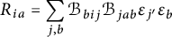 $$\begin{align*}R_{ia} = \sum_{j,b} \mathcal{B}_{bij} \mathcal{B}_{jab}\varepsilon_{j'}\varepsilon_b \end{align*}$$
of the Ricci curvature (for zero divergence
 $\delta =0$
) with respect to the orthonormal basis
$\delta =0$
) with respect to the orthonormal basis
 $(e_A)=(e_a,e_i)$
,
$(e_A)=(e_a,e_i)$
,
 $e_a = v_a + gv_a$
,
$e_a = v_a + gv_a$
,
 $e_i=v_{i'}-gv_{i'}$
, of
$e_i=v_{i'}-gv_{i'}$
, of
 $E=\mathfrak g \oplus \mathfrak g^*$
. Explicitly, we obtain
$E=\mathfrak g \oplus \mathfrak g^*$
. Explicitly, we obtain
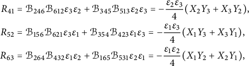 $$ \begin{align*} R_{41} &= \mathcal{B}_{246}\mathcal{B}_{612}\varepsilon_3\varepsilon_2 + \mathcal{B}_{345}\mathcal{B}_{513}\varepsilon_2\varepsilon_3=-\frac{\varepsilon_2\varepsilon_3}{4}(X_2Y_3+X_3Y_2),\\ R_{52}&=\mathcal{B}_{156} \mathcal{B}_{621}\varepsilon_{3}\varepsilon_1 + \mathcal{B}_{354} \mathcal{B}_{423}\varepsilon_{1}\varepsilon_3= -\frac{\varepsilon_1\varepsilon_3}{4}(X_1Y_3+X_3Y_1),\\ R_{63}&= \mathcal{B}_{264} \mathcal{B}_{432}\varepsilon_{1}\varepsilon_2 + \mathcal{B}_{165} \mathcal{B}_{531}\varepsilon_{2}\varepsilon_1 =-\frac{\varepsilon_1\varepsilon_2}{4}(X_1Y_2+X_2Y_1), \end{align*} $$
with all other components equal to zero. We conclude that the generalized Einstein equations reduce to a system of three homogeneous quadratic equations in the variables
 $X_a$
and
$X_a$
and
 $Y_a$
:
$Y_a$
:
 $$\begin{align*}X_1Y_2+X_2Y_1=X_1Y_3+X_3Y_1=X_2Y_3+X_3Y_2=0.\end{align*}$$
A priori, we can distinguish four types of solutions depending on how many components of the vector
 $(X_1,X_2,X_3)$
are equal to zero: 0, 1, 2, or 3.
$(X_1,X_2,X_3)$
are equal to zero: 0, 1, 2, or 3.
Solutions of type
 $0$
:
$0$
:
 $X_1X_2X_3\neq 0$
implies
$X_1X_2X_3\neq 0$
implies
 $Y_1=Y_2=Y_3=0$
and finally
$Y_1=Y_2=Y_3=0$
and finally
 $$\begin{align*}\alpha_1=\alpha_2=\alpha_3=-h\neq0.\end{align*}$$
In this case, the Lie algebra
 $\mathfrak g$
is isomorphic to
$\mathfrak g$
is isomorphic to
 $\mathfrak {so}(2,1)$
or
$\mathfrak {so}(2,1)$
or
 $\mathfrak {so}(3)$
. The latter case happens if and only if the metric g is definite.
$\mathfrak {so}(3)$
. The latter case happens if and only if the metric g is definite.
Solutions of type
 $1$
: assume, for example, that
$1$
: assume, for example, that
 $X_1X_2\neq 0$
,
$X_1X_2\neq 0$
,
 $X_3=0$
. This implies that
$X_3=0$
. This implies that
 $Y_3=0$
and, hence,
$Y_3=0$
and, hence,
 $\alpha _3=\alpha _1+\alpha _2$
and
$\alpha _3=\alpha _1+\alpha _2$
and
 $h=0$
. But then, the equation
$h=0$
. But then, the equation
 $X_1Y_2+X_2Y_1=0$
reduces to
$X_1Y_2+X_2Y_1=0$
reduces to
 $\alpha _1\alpha _2=0$
, which is inconsistent with
$\alpha _1\alpha _2=0$
, which is inconsistent with
 $X_1X_2\neq 0$
. This shows that solutions of type
$X_1X_2\neq 0$
. This shows that solutions of type
 $1$
do not exist.
$1$
do not exist.
Solutions of type
 $2$
: assume, for example, that
$2$
: assume, for example, that
 $X_1\neq 0$
,
$X_1\neq 0$
,
 $X_2=X_3=0$
. This implies
$X_2=X_3=0$
. This implies
 $Y_2=Y_3=0$
and finally
$Y_2=Y_3=0$
and finally
 $h=\alpha _1=0$
,
$h=\alpha _1=0$
,
 $\alpha _2=\alpha _3\neq 0$
. So the solutions of type
$\alpha _2=\alpha _3\neq 0$
. So the solutions of type
 $2$
are of the following form. There exists a cyclic permutation
$2$
are of the following form. There exists a cyclic permutation
 $\sigma \in \mathfrak {S}_3$
such that
$\sigma \in \mathfrak {S}_3$
such that
 $$\begin{align*}\alpha_{\sigma (1)}=\alpha_{\sigma (2)}\neq0\quad\mbox{and}\quad h=\alpha_{\sigma (3)}=0.\end{align*}$$
We conclude, for solutions of type 2, that g is flat (see Corollary 2.31) and
 $\mathfrak g$
is metabelian.
$\mathfrak g$
is metabelian.
 $[\mathfrak g,\mathfrak g]= \mathrm {span}\{ v_{\sigma (1)},v_{\sigma (2)}\}$
is two-dimensional and
$[\mathfrak g,\mathfrak g]= \mathrm {span}\{ v_{\sigma (1)},v_{\sigma (2)}\}$
is two-dimensional and
 $\mathrm {ad}_{v_{\sigma (3)}}$
acts on it by a nonzero g-skew-symmetric endomorphism. This implies that
$\mathrm {ad}_{v_{\sigma (3)}}$
acts on it by a nonzero g-skew-symmetric endomorphism. This implies that
 $\mathfrak g$
is isomorphic to
$\mathfrak g$
is isomorphic to
 $\mathfrak {e}(2)$
or
$\mathfrak {e}(2)$
or
 $\mathfrak {e}(1,1)$
.
$\mathfrak {e}(1,1)$
.
Solutions of type
 $3$
: assume
$3$
: assume
 $X_1=X_2=X_3=0$
. This implies
$X_1=X_2=X_3=0$
. This implies
 $$\begin{align*}\alpha_1=\alpha_2=\alpha_3=h.\end{align*}$$
In this case,
 $\mathfrak g$
is either abelian and g is flat (the case
$\mathfrak g$
is either abelian and g is flat (the case
 $h=0$
again by Corollary 2.31) or
$h=0$
again by Corollary 2.31) or
 $\mathfrak g$
is isomorphic to
$\mathfrak g$
is isomorphic to
 $\mathfrak {so}(2,1)$
or
$\mathfrak {so}(2,1)$
or
 $\mathfrak {so}(3)$
, as for type
$\mathfrak {so}(3)$
, as for type
 $ 0 $
.
$ 0 $
.
If
 $ L $
is not diagonalizable, then
$ L $
is not diagonalizable, then
 $ g $
is indefinite and there exists an orthonormal basis
$ g $
is indefinite and there exists an orthonormal basis
 $ (v_a)_a $
with
$ (v_a)_a $
with
 $g(v_1,v_1)=g(v_2,v_2)=-g(v_3,v_3)$
such that
$g(v_1,v_1)=g(v_2,v_2)=-g(v_3,v_3)$
such that
 $ L $
is either of the form
$ L $
is either of the form
 $ L_3(0,0) $
or
$ L_3(0,0) $
or
 $ L_4(0,0) $
, and
$ L_4(0,0) $
, and
 $ h=0 $
by Proposition 3.3. We consider first the case
$ h=0 $
by Proposition 3.3. We consider first the case
 $ L_3(0,0) $
. To prove that
$ L_3(0,0) $
. To prove that
 $ G $
is isomorphic to the Heisenberg group, we show, using equation (25), that the generators
$ G $
is isomorphic to the Heisenberg group, we show, using equation (25), that the generators
![]() and
and
![]() of its Lie algebra
of its Lie algebra
 $ \mathfrak {g} $
satisfy the relations
$ \mathfrak {g} $
satisfy the relations
 $ [P, Q] = R $
and
$ [P, Q] = R $
and
 $[P, R] = [Q, R] = 0 $
:
$[P, R] = [Q, R] = 0 $
:
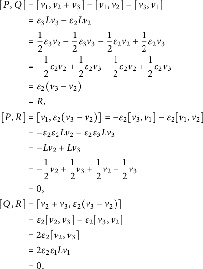 $$ \begin{align*} \left[P,Q\right]&=[v_1,v_2+v_3]=[v_1,v_2]-[v_3,v_1]\\ &=\varepsilon_3Lv_3-\varepsilon_2Lv_2\\ &=\frac12\varepsilon_3v_2-\frac12\varepsilon_3v_3-\frac12\varepsilon_2v_2+\frac12\varepsilon_2v_3\\ &=-\frac12\varepsilon_2v_2+\frac12\varepsilon_2v_3-\frac12\varepsilon_2v_2+\frac12\varepsilon_2v_3\\ &=\varepsilon_2(v_3-v_2)\\ &=R,\\ \left[P,R\right]&=[v_1,\varepsilon_2(v_3-v_2)]=-\varepsilon_2[v_3,v_1]-\varepsilon_2[v_1,v_2]\\ &=-\varepsilon_2\varepsilon_2Lv_2-\varepsilon_2\varepsilon_3Lv_3\\ &=-Lv_2+Lv_3\\ &=-\frac12v_2+\frac12v_3+\frac12v_2-\frac12v_3\\ &=0,\\ \left[Q,R\right]&=[v_2+v_3,\varepsilon_2(v_3-v_2)]\\ &=\varepsilon_2[v_2,v_3]-\varepsilon_2[v_3,v_2]\\ &=2\varepsilon_2[v_2,v_3]\\ &=2\varepsilon_2\varepsilon_1Lv_1\\ &=0. \end{align*} $$
In the case that
 $ L $
takes the form
$ L $
takes the form
 $ L_4(0,0) $
, we see analogously that the generators
$ L_4(0,0) $
, we see analogously that the generators
 $ P=v_1, Q=v_2+v_3 $
and
$ P=v_1, Q=v_2+v_3 $
and
 $ R=\varepsilon _2(v_2-v_3) $
satisfy the relations
$ R=\varepsilon _2(v_2-v_3) $
satisfy the relations
 $ [P, Q] = R $
and
$ [P, Q] = R $
and
 $[P, R] = [Q, R] = 0 $
.
$[P, R] = [Q, R] = 0 $
.
3.2.2 Nonunimodular Lie groups
We assume now that the Lie group
 $ G $
is not unimodular. Let
$ G $
is not unimodular. Let
![]() be the unimodular kernel of
be the unimodular kernel of
 $ \mathfrak {g} $
. It can be easily checked that
$ \mathfrak {g} $
. It can be easily checked that
 $ \mathfrak {u} $
is a two-dimensional abelian ideal of
$ \mathfrak {u} $
is a two-dimensional abelian ideal of
 $ \mathfrak {g} $
, containing the commutator ideal
$ \mathfrak {g} $
, containing the commutator ideal
 $ [\mathfrak {g},\mathfrak {g}] $
. This means that the Lie algebra
$ [\mathfrak {g},\mathfrak {g}] $
. This means that the Lie algebra
 $ \mathfrak {g} $
is a semidirect product of
$ \mathfrak {g} $
is a semidirect product of
 $ \mathbb {R} $
and
$ \mathbb {R} $
and
 $ \mathbb {R}^2 $
, where
$ \mathbb {R}^2 $
, where
 $ \mathbb {R} $
is acting on
$ \mathbb {R} $
is acting on
 $ \mathbb {R}^2 $
by an endomorphism with nonzero trace. For details on the classification of nonunimodular, three-dimensional Lie algebras in terms of the Jordan normal form of this endomorphism, we refer to [Reference Gorbatsevich, Onishchik and VinbergGOV, Chapter 7, Theorem 1.4].
$ \mathbb {R}^2 $
by an endomorphism with nonzero trace. For details on the classification of nonunimodular, three-dimensional Lie algebras in terms of the Jordan normal form of this endomorphism, we refer to [Reference Gorbatsevich, Onishchik and VinbergGOV, Chapter 7, Theorem 1.4].
We first treat the case that the restriction
 $ g|_{\mathfrak {u}\times \mathfrak {u}} $
of the metric
$ g|_{\mathfrak {u}\times \mathfrak {u}} $
of the metric
 $ g $
to
$ g $
to
 $ \mathfrak {u} $
is nondegenerate.
$ \mathfrak {u} $
is nondegenerate.
Proposition 3.5 Let
 $(H,\mathcal G_g,\delta =0)$
be a divergence-free generalized Einstein structure on a three-dimensional nonunimodular Lie group G. Let
$(H,\mathcal G_g,\delta =0)$
be a divergence-free generalized Einstein structure on a three-dimensional nonunimodular Lie group G. Let
 $ \mathfrak {u} $
be the unimodular kernel of the Lie algebra
$ \mathfrak {u} $
be the unimodular kernel of the Lie algebra
 $ \mathfrak {g} $
and assume that
$ \mathfrak {g} $
and assume that
 $ g|_{\mathfrak {u}\times \mathfrak {u}} $
is nondegenerate. Then
$ g|_{\mathfrak {u}\times \mathfrak {u}} $
is nondegenerate. Then
 $ H=0 $
and
$ H=0 $
and
 $ g $
is indefinite. Furthermore, there exists an orthonormal basis
$ g $
is indefinite. Furthermore, there exists an orthonormal basis
 $(v_a)$
of
$(v_a)$
of
 $(\mathfrak {g},g)$
such that
$(\mathfrak {g},g)$
such that
 $ v_1,v_3\in \mathfrak {u} $
and
$ v_1,v_3\in \mathfrak {u} $
and
 $g(v_1,v_1)=g(v_2,v_2)=-g(v_3,v_3)$
and a positive constant
$g(v_1,v_1)=g(v_2,v_2)=-g(v_3,v_3)$
and a positive constant
 $ \theta>0 $
such that
$ \theta>0 $
such that
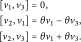 $$ \begin{align*} [v_1,v_3]&=0,\\ \left[v_2,v_1\right]&=\theta v_1-\theta v_3,\\ \left[v_2,v_3\right]&=\theta v_1+\theta v_3. \end{align*} $$
Proof A
 $ g $
-orthonormal basis
$ g $
-orthonormal basis
 $ (v_a)_a $
of
$ (v_a)_a $
of
 $ \mathfrak g $
such that
$ \mathfrak g $
such that
 $ v_1,v_3\in \mathfrak {u} $
exists, because
$ v_1,v_3\in \mathfrak {u} $
exists, because
 $ g|_{\mathfrak {u}\times \mathfrak {u}} $
is nondegenerate. Since
$ g|_{\mathfrak {u}\times \mathfrak {u}} $
is nondegenerate. Since
 $ \mathfrak {u} $
is an abelian ideal, there are
$ \mathfrak {u} $
is an abelian ideal, there are
 $ \lambda ,\mu ,\nu ,\rho \in \mathbb {R}$
such that
$ \lambda ,\mu ,\nu ,\rho \in \mathbb {R}$
such that
 $$ \begin{align*} [v_3,v_1]&=0,\\ \left[v_2,v_1\right]&=\varepsilon_1\lambda v_1+\varepsilon_3\mu v_3,\\ \left[v_2,v_3\right]&=\varepsilon_1\nu v_1+\varepsilon_{3}\rho v_3, \end{align*} $$
with
 $ 0\neq \operatorname {\mathrm{tr}} \mathrm {ad}_{v_2}=\varepsilon _1\lambda +\varepsilon _{3}\rho $
. Using
$ 0\neq \operatorname {\mathrm{tr}} \mathrm {ad}_{v_2}=\varepsilon _1\lambda +\varepsilon _{3}\rho $
. Using
 $ \lambda =\kappa _{211},\mu =\kappa _{213},\nu =\kappa _{231} $
and
$ \lambda =\kappa _{211},\mu =\kappa _{213},\nu =\kappa _{231} $
and
 $ \rho =\kappa _{233} $
, we can compute the Dorfman coefficients
$ \rho =\kappa _{233} $
, we can compute the Dorfman coefficients
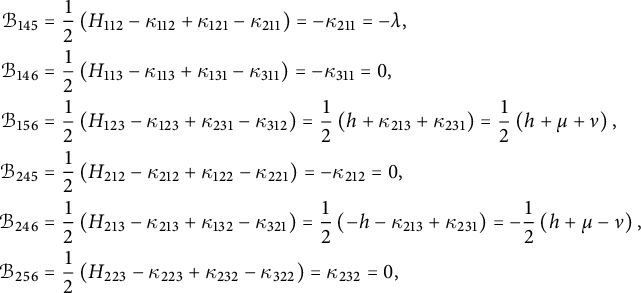 $$ \begin{align*} \mathcal B_{145}&=\frac12\left(H_{112}-\kappa_{112}+\kappa_{121}-\kappa_{211}\right)=-\kappa_{211}=-\lambda,\\ \mathcal B_{146}&=\frac12\left(H_{113}-\kappa_{113}+\kappa_{131}-\kappa_{311}\right)=-\kappa_{311}=0,\\ \mathcal B_{156}&=\frac12\left(H_{123}-\kappa_{123}+\kappa_{231}-\kappa_{312}\right)=\frac12\left(h+\kappa_{213}+\kappa_{231}\right)=\frac12\left(h+\mu+\nu\right),\\ \mathcal B_{245}&=\frac12\left(H_{212}-\kappa_{212}+\kappa_{122}-\kappa_{221}\right)=-\kappa_{212}=0,\\ \mathcal B_{246}&=\frac12\left(H_{213}-\kappa_{213}+\kappa_{132}-\kappa_{321}\right)=\frac12\left(-h-\kappa_{213}+\kappa_{231}\right)=-\frac12\left(h+\mu-\nu\right),\\ \mathcal B_{256}&=\frac12\left(H_{223}-\kappa_{223}+\kappa_{232}-\kappa_{322}\right)=\kappa_{232}=0, \end{align*} $$
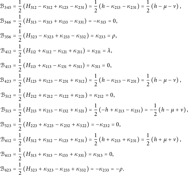 $$ \begin{align*} \mathcal B_{345}&=\frac12\left(H_{312}-\kappa_{312}+\kappa_{123}-\kappa_{231}\right)=\frac12\left(h-\kappa_{213}-\kappa_{231}\right)=\frac12\left(h-\mu-\nu\right),\\ \mathcal B_{346}&=\frac12\left(H_{313}-\kappa_{313}+\kappa_{133}-\kappa_{331}\right)=-\kappa_{313}=0,\\ \mathcal B_{356}&=\frac12\left(H_{323}-\kappa_{323}+\kappa_{233}-\kappa_{332}\right)=\kappa_{233}=\rho,\\ \mathcal B_{412}&=\frac12\left(H_{112}+\kappa_{112}-\kappa_{121}+\kappa_{211}\right)=\kappa_{211}=\lambda,\\ \mathcal B_{413}&=\frac12\left(H_{113}+\kappa_{113}-\kappa_{131}+\kappa_{311}\right)=\kappa_{311}=0,\\ \mathcal B_{423}&=\frac12\left(H_{123}+\kappa_{123}-\kappa_{231}+\kappa_{312}\right)=\frac12\left(h-\kappa_{213}-\kappa_{231}\right)=\frac12\left(h-\mu-\nu\right),\\ \mathcal B_{512}&=\frac12\left(H_{212}+\kappa_{212}-\kappa_{122}+\kappa_{221}\right)=\kappa_{212}=0,\\ \mathcal B_{513}&=\frac12\left(H_{213}+\kappa_{213}-\kappa_{132}+\kappa_{321}\right)=\frac12\left(-h+\kappa_{213}-\kappa_{231}\right)=-\frac12\left(h-\mu+\nu\right),\\ \mathcal B_{523}&=\frac12\left(H_{223}+\kappa_{223}-\kappa_{232}+\kappa_{322}\right)=-\kappa_{232}=0,\\ \mathcal B_{612}&=\frac12\left(H_{312}+\kappa_{312}-\kappa_{123}+\kappa_{231}\right)=\frac12\left(h+\kappa_{213}+\kappa_{231}\right)=\frac12\left(h+\mu+\nu\right),\\ \mathcal B_{613}&=\frac12\left(H_{313}+\kappa_{313}-\kappa_{133}+\kappa_{331}\right)=\kappa_{313}=0,\\ \mathcal B_{623}&=\frac12\left(H_{323}+\kappa_{323}-\kappa_{233}+\kappa_{332}\right)=-\kappa_{233}=-\rho. \end{align*} $$
To prove that the case
 $\varepsilon _1=\varepsilon _3$
cannot occur, we compute using equation (26),
$\varepsilon _1=\varepsilon _3$
cannot occur, we compute using equation (26),
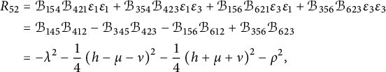 $$ \begin{align*} R_{52}&=\mathcal{B}_{154}\mathcal{B}_{421}\varepsilon_{1}\varepsilon_1+\mathcal{B}_{354}\mathcal{B}_{423}\varepsilon_{1}\varepsilon_3+\mathcal{B}_{156}\mathcal{B}_{621}\varepsilon_{3}\varepsilon_1+\mathcal{B}_{356}\mathcal{B}_{623}\varepsilon_{3}\varepsilon_3\\ &=\mathcal{B}_{145}\mathcal{B}_{412}-\mathcal{B}_{345}\mathcal{B}_{423}-\mathcal{B}_{156}\mathcal{B}_{612}+\mathcal{B}_{356}\mathcal{B}_{623}\\ &=-\lambda^2-\frac14\left(h-\mu-\nu\right)^2-\frac14\left(h+\mu+\nu\right)^2-\rho^2, \end{align*} $$
where we have used that
 $ \varepsilon _{1}=\varepsilon _{3} $
. But this can only be zero if
$ \varepsilon _{1}=\varepsilon _{3} $
. But this can only be zero if
 $ \lambda =\rho =0 $
, which contradicts
$ \lambda =\rho =0 $
, which contradicts
 $ 0\neq \operatorname {\mathrm{tr}} \mathrm {ad}_{v_2}=\varepsilon _1\lambda +\varepsilon _{3}\rho $
. This proves that
$ 0\neq \operatorname {\mathrm{tr}} \mathrm {ad}_{v_2}=\varepsilon _1\lambda +\varepsilon _{3}\rho $
. This proves that
 $\varepsilon _1=-\varepsilon _3$
. Hence, we can assume that the basis is chosen such that
$\varepsilon _1=-\varepsilon _3$
. Hence, we can assume that the basis is chosen such that
 $ \varepsilon _{1}=\varepsilon _{2}=-\varepsilon _{3} $
.
$ \varepsilon _{1}=\varepsilon _{2}=-\varepsilon _{3} $
.
In this case, the components of the Ricci curvature are
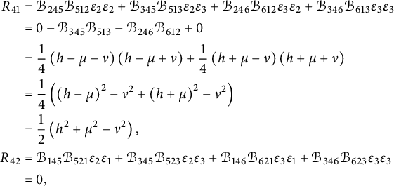 $$ \begin{align*} R_{41}&=\mathcal{B}_{245}\mathcal{B}_{512}\varepsilon_{2}\varepsilon_2+\mathcal{B}_{345}\mathcal{B}_{513}\varepsilon_{2}\varepsilon_3+\mathcal{B}_{246}\mathcal{B}_{612}\varepsilon_{3}\varepsilon_2+\mathcal{B}_{346}\mathcal{B}_{613}\varepsilon_{3}\varepsilon_3\\ &=0-\mathcal{B}_{345}\mathcal{B}_{513}-\mathcal{B}_{246}\mathcal{B}_{612}+0\\ &=\frac14\left(h-\mu-\nu\right)\left(h-\mu+\nu\right)+\frac14\left(h+\mu-\nu\right)\left(h+\mu+\nu\right)\\ &=\frac14\left(\left(h-\mu\right)^2-\nu^2+\left(h+\mu\right)^2-\nu^2\right)\\ &=\frac12\left(h^2+\mu^2-\nu^2\right),\\ R_{42}&=\mathcal{B}_{145}\mathcal{B}_{521}\varepsilon_{2}\varepsilon_1+\mathcal{B}_{345}\mathcal{B}_{523}\varepsilon_{2}\varepsilon_3+\mathcal{B}_{146}\mathcal{B}_{621}\varepsilon_{3}\varepsilon_1+\mathcal{B}_{346}\mathcal{B}_{623}\varepsilon_{3}\varepsilon_3\\ &=0, \end{align*} $$
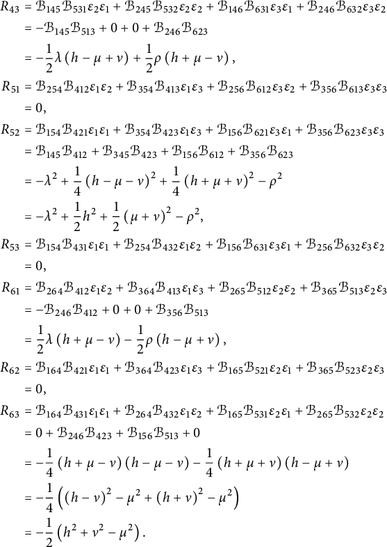 $$ \begin{align*} R_{43}&=\mathcal{B}_{145}\mathcal{B}_{531}\varepsilon_{2}\varepsilon_1+\mathcal{B}_{245}\mathcal{B}_{532}\varepsilon_{2}\varepsilon_2+\mathcal{B}_{146}\mathcal{B}_{631}\varepsilon_{3}\varepsilon_1+\mathcal{B}_{246}\mathcal{B}_{632}\varepsilon_{3}\varepsilon_2\\ &=-\mathcal{B}_{145}\mathcal{B}_{513}+0+0+\mathcal{B}_{246}\mathcal{B}_{623}\\ &=-\frac12\lambda\left(h-\mu+\nu\right)+\frac12\rho\left(h+\mu-\nu\right),\\ R_{51}&=\mathcal{B}_{254}\mathcal{B}_{412}\varepsilon_{1}\varepsilon_2+\mathcal{B}_{354}\mathcal{B}_{413}\varepsilon_{1}\varepsilon_3+\mathcal{B}_{256}\mathcal{B}_{612}\varepsilon_{3}\varepsilon_2+\mathcal{B}_{356}\mathcal{B}_{613}\varepsilon_{3}\varepsilon_3\\ &=0,\\ R_{52}&=\mathcal{B}_{154}\mathcal{B}_{421}\varepsilon_{1}\varepsilon_1+\mathcal{B}_{354}\mathcal{B}_{423}\varepsilon_{1}\varepsilon_3+\mathcal{B}_{156}\mathcal{B}_{621}\varepsilon_{3}\varepsilon_1+\mathcal{B}_{356}\mathcal{B}_{623}\varepsilon_{3}\varepsilon_3\\ &=\mathcal{B}_{145}\mathcal{B}_{412}+\mathcal{B}_{345}\mathcal{B}_{423}+\mathcal{B}_{156}\mathcal{B}_{612}+\mathcal{B}_{356}\mathcal{B}_{623}\\ &=-\lambda^2+\frac14\left(h-\mu-\nu\right)^2+\frac14\left(h+\mu+\nu\right)^2-\rho^2\\ &=-\lambda^2+\frac12h^2+\frac12\left(\mu+\nu\right)^2-\rho^2,\\ R_{53}&=\mathcal{B}_{154}\mathcal{B}_{431}\varepsilon_{1}\varepsilon_1+\mathcal{B}_{254}\mathcal{B}_{432}\varepsilon_{1}\varepsilon_2+\mathcal{B}_{156}\mathcal{B}_{631}\varepsilon_{3}\varepsilon_1+\mathcal{B}_{256}\mathcal{B}_{632}\varepsilon_{3}\varepsilon_2\\ &=0,\\ R_{61}&=\mathcal{B}_{264}\mathcal{B}_{412}\varepsilon_{1}\varepsilon_2+\mathcal{B}_{364}\mathcal{B}_{413}\varepsilon_{1}\varepsilon_3+\mathcal{B}_{265}\mathcal{B}_{512}\varepsilon_{2}\varepsilon_2+\mathcal{B}_{365}\mathcal{B}_{513}\varepsilon_{2}\varepsilon_3\\ &=-\mathcal{B}_{246}\mathcal{B}_{412}+0+0+\mathcal{B}_{356}\mathcal{B}_{513}\\ &=\frac12\lambda\left(h+\mu-\nu\right)-\frac12\rho\left(h-\mu+\nu\right),\\ R_{62}&=\mathcal{B}_{164}\mathcal{B}_{421}\varepsilon_{1}\varepsilon_1+\mathcal{B}_{364}\mathcal{B}_{423}\varepsilon_{1}\varepsilon_3+\mathcal{B}_{165}\mathcal{B}_{521}\varepsilon_{2}\varepsilon_1+\mathcal{B}_{365}\mathcal{B}_{523}\varepsilon_{2}\varepsilon_3\\ &=0,\\ R_{63}&=\mathcal{B}_{164}\mathcal{B}_{431}\varepsilon_{1}\varepsilon_1+\mathcal{B}_{264}\mathcal{B}_{432}\varepsilon_{1}\varepsilon_2+\mathcal{B}_{165}\mathcal{B}_{531}\varepsilon_{2}\varepsilon_1+\mathcal{B}_{265}\mathcal{B}_{532}\varepsilon_{2}\varepsilon_2\\ &=0+\mathcal{B}_{246}\mathcal{B}_{423}+\mathcal{B}_{156}\mathcal{B}_{513}+0\\ &=-\frac14\left(h+\mu-\nu\right)\left(h-\mu-\nu\right)-\frac14\left(h+\mu+\nu\right)\left(h-\mu+\nu\right)\\ &=-\frac14\left(\left(h-\nu\right)^2-\mu^2+\left(h+\nu\right)^2-\mu^2\right)\\ &=-\frac12\left(h^2+\nu^2-\mu^2\right). \end{align*} $$
Imposing the Einstein condition, we see from the equations
 $ R_{41}+R_{63}=0 $
and
$ R_{41}+R_{63}=0 $
and
 $ R_{41}-R_{63}=0 $
, that
$ R_{41}-R_{63}=0 $
, that
 $ h^2=0 $
and
$ h^2=0 $
and
 $ \mu ^2=\nu ^2 $
. If
$ \mu ^2=\nu ^2 $
. If
 $ \mu =-\nu $
, then
$ \mu =-\nu $
, then
 $ R_{52}=0 $
reads as
$ R_{52}=0 $
reads as
 $ 0=-\lambda ^2-\rho ^2 $
, hence
$ 0=-\lambda ^2-\rho ^2 $
, hence
 $ \lambda =\rho =0 $
, which contradicts
$ \lambda =\rho =0 $
, which contradicts
 $ 0\neq \operatorname {\mathrm{tr}} \mathrm {ad}_{v_2}=\varepsilon _1\lambda +\varepsilon _{3}\rho $
. Therefore,
$ 0\neq \operatorname {\mathrm{tr}} \mathrm {ad}_{v_2}=\varepsilon _1\lambda +\varepsilon _{3}\rho $
. Therefore,
 $ \mu =\nu $
and, from
$ \mu =\nu $
and, from
 $ R_{52}=0 $
,
$ R_{52}=0 $
,
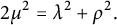 $$\begin{align*}2\mu^2=\lambda^2+\rho^2. \end{align*}$$
In particular,
 $ \mu \neq 0 $
, due to
$ \mu \neq 0 $
, due to
 $ 0\neq \operatorname {\mathrm{tr}} \mathrm {ad}_{v_2}=\varepsilon _1\lambda +\varepsilon _{3}\rho $
. Note now that
$ 0\neq \operatorname {\mathrm{tr}} \mathrm {ad}_{v_2}=\varepsilon _1\lambda +\varepsilon _{3}\rho $
. Note now that
 $ \mu =\nu $
implies that the endomorphism
$ \mu =\nu $
implies that the endomorphism
 $ M\in \operatorname {\mathrm {End}}(\mathfrak {u}) $
, defined as the restriction of
$ M\in \operatorname {\mathrm {End}}(\mathfrak {u}) $
, defined as the restriction of
 $ \mathrm {ad}_{v_2} $
to
$ \mathrm {ad}_{v_2} $
to
 $ \mathfrak {u} $
, is symmetric. A simple consequence of [Reference Cortés, Ehlert, Haupt and LindemannCEHL, Lemma 2.2] (compare Proposition 3.2) is that there exists an orthonormal basis of
$ \mathfrak {u} $
, is symmetric. A simple consequence of [Reference Cortés, Ehlert, Haupt and LindemannCEHL, Lemma 2.2] (compare Proposition 3.2) is that there exists an orthonormal basis of
 $ \mathfrak {u} $
such that
$ \mathfrak {u} $
such that
 $ M $
is represented by one of the matrices
$ M $
is represented by one of the matrices
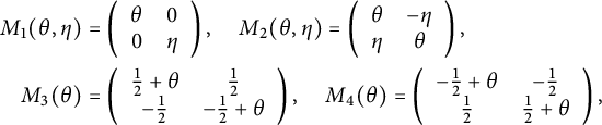 $$ \begin{align*} M_1(\theta,\eta ) &= \left( \begin{array}{cc} \theta& 0\\ 0&\eta \end{array}\right),\quad M_2(\theta,\eta )=\left( \begin{array}{cc} \theta& -\eta\\ \eta&\theta \end{array}\right),\\ M_3(\theta)&=\left( \begin{array}{cc}\frac12+\theta &\frac12\\ -\frac12&-\frac12 +\theta \end{array}\right),\quad M_4(\theta)= \left( \begin{array}{cc} -\frac12+\theta &-\frac12\\ \frac12&\frac12 +\theta\\ \end{array}\right), \end{align*} $$
in this basis. We may assume that the basis
 $ v_1,v_3 $
of
$ v_1,v_3 $
of
 $ \mathfrak {u} $
is chosen such that
$ \mathfrak {u} $
is chosen such that
 $ M $
takes one of these normal forms with respect to
$ M $
takes one of these normal forms with respect to
 $ v_1,v_3 $
. We see that
$ v_1,v_3 $
. We see that
 $ M_1(\theta ,\eta ) $
is excluded by the condition
$ M_1(\theta ,\eta ) $
is excluded by the condition
 $ \mu \neq 0 $
. Applying
$ \mu \neq 0 $
. Applying
 $ 2\mu ^2=\lambda ^2+\rho ^2 $
to the normal form
$ 2\mu ^2=\lambda ^2+\rho ^2 $
to the normal form
 $ M_3(\theta ) $
yields
$ M_3(\theta ) $
yields
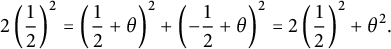 $$\begin{align*}2\left(\frac12\right)^2=\left(\frac12+\theta\right)^2+ \left(-\frac12+\theta\right)^2=2\left(\frac12\right)^2+\theta^2. \end{align*}$$
Hence,
 $ \theta =0 $
, which contradicts
$ \theta =0 $
, which contradicts
 $ \operatorname {\mathrm{tr}} \mathrm {ad}_{v_2}\neq 0 $
. For the same reason,
$ \operatorname {\mathrm{tr}} \mathrm {ad}_{v_2}\neq 0 $
. For the same reason,
 $ M $
also cannot have the normal form
$ M $
also cannot have the normal form
 $ M_4(\theta ) $
. In the remaining case
$ M_4(\theta ) $
. In the remaining case
 $ M_2(\theta ,\eta ), $
the equation
$ M_2(\theta ,\eta ), $
the equation
 $ 2\mu ^2=\lambda ^2+\rho ^2 $
reads as
$ 2\mu ^2=\lambda ^2+\rho ^2 $
reads as
 $ 2\left (-\eta \right )^2=\theta ^2+\left (-\theta \right )^2 $
. Therefore,
$ 2\left (-\eta \right )^2=\theta ^2+\left (-\theta \right )^2 $
. Therefore,
 $ \eta =\pm \theta $
. Furthermore,
$ \eta =\pm \theta $
. Furthermore,
 $ \eta \neq 0 $
because
$ \eta \neq 0 $
because
 $ \mu \neq 0 $
. Hence, the only two normal forms are
$ \mu \neq 0 $
. Hence, the only two normal forms are
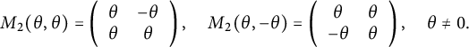 $$ \begin{align*} M_2(\theta,\theta )=\left( \begin{array}{cc} \theta& -\theta\\ \theta&\theta \end{array}\right),\quad M_2(\theta,-\theta )=\left( \begin{array}{cc} \theta& \theta\\ -\theta&\theta \end{array}\right),\quad \theta\neq0. \end{align*} $$
Replacing
 $ v_1 $
by
$ v_1 $
by
 $ -v_1 $
(exchanging
$ -v_1 $
(exchanging
 $ M_2(\theta ,\theta ) $
with
$ M_2(\theta ,\theta ) $
with
 $ M_2(\theta ,-\theta ) $
) and
$ M_2(\theta ,-\theta ) $
) and
 $ v_2 $
by
$ v_2 $
by
 $ -v_2 $
(replacing
$ -v_2 $
(replacing
 $ \theta $
by
$ \theta $
by
 $ -\theta $
), if necessary, we obtain the claimed equations for
$ -\theta $
), if necessary, we obtain the claimed equations for
 $ \theta>0 $
.
$ \theta>0 $
.
Remark 3.6 Note that, while all the occurring Lie algebras in the previous proposition are nonisomorphic as metric Lie algebras, they are isomorphic as Lie algebras. They are a semidirect product of
 $ \mathbb {R}^2 $
and
$ \mathbb {R}^2 $
and
 $ \mathbb {R} $
, where
$ \mathbb {R} $
, where
 $ \mathbb {R} $
acts on
$ \mathbb {R} $
acts on
 $ \mathbb {R}^2 $
by the endomorphism
$ \mathbb {R}^2 $
by the endomorphism
 $ \mathrm {ad}_{v_2}|_{\mathfrak {u}} $
, which has nonreal and nonimaginary eigenvalues
$ \mathrm {ad}_{v_2}|_{\mathfrak {u}} $
, which has nonreal and nonimaginary eigenvalues
 $ (1+i)\theta $
and
$ (1+i)\theta $
and
 $ (1-i)\theta $
. This corresponds to the Lie algebra
$ (1-i)\theta $
. This corresponds to the Lie algebra
 $ \mathfrak {r}^{\prime }_{3,1}(\mathbb {R}) $
in the notation of [Reference Gorbatsevich, Onishchik and VinbergGOV, Chapter 7, Theorem 1.4].
$ \mathfrak {r}^{\prime }_{3,1}(\mathbb {R}) $
in the notation of [Reference Gorbatsevich, Onishchik and VinbergGOV, Chapter 7, Theorem 1.4].
Proposition 3.7 There is no divergence-free generalized Einstein structure
 $(H,\mathcal G_g,\delta =0)$
on a three-dimensional nonunimodular Lie group G such that
$(H,\mathcal G_g,\delta =0)$
on a three-dimensional nonunimodular Lie group G such that
 $ g $
is degenerate on the unimodular kernel
$ g $
is degenerate on the unimodular kernel
 $ \mathfrak {u} $
of
$ \mathfrak {u} $
of
 $ \mathfrak {g} $
.
$ \mathfrak {g} $
.
Proof Note first that the metric
 $ g $
necessarily has to be indefinite. We define
$ g $
necessarily has to be indefinite. We define
![]() if the signature of
if the signature of
 $ g $
is
$ g $
is
 $ (2,1) $
and
$ (2,1) $
and
![]() if it is
if it is
 $ (1,2) $
. Note that in both cases, there is a two-dimensional subspace of
$ (1,2) $
. Note that in both cases, there is a two-dimensional subspace of
 $\mathfrak {g}$
on which
$\mathfrak {g}$
on which
 $\varepsilon g$
is positive definite. Taking the intersection with
$\varepsilon g$
is positive definite. Taking the intersection with
 $\mathfrak {u}$
, we obtain a one-dimensional subspace generated by a vector
$\mathfrak {u}$
, we obtain a one-dimensional subspace generated by a vector
 $w_1$
such that
$w_1$
such that
 $g(w_1,w_1)=\varepsilon $
. Next, we choose a generator
$g(w_1,w_1)=\varepsilon $
. Next, we choose a generator
 $w_2$
of the kernel of
$w_2$
of the kernel of
 $g|_{\mathfrak {u} \times \mathfrak {u}}$
and a null vector
$g|_{\mathfrak {u} \times \mathfrak {u}}$
and a null vector
 $w_3$
orthogonal to
$w_3$
orthogonal to
 $w_1$
such that
$w_1$
such that
 $g(w_2,w_3)=\frac \varepsilon 2$
. Summarizing, we obtain a basis
$g(w_2,w_3)=\frac \varepsilon 2$
. Summarizing, we obtain a basis
 $(w_a)$
of
$(w_a)$
of
 $\mathfrak {g}$
such that
$\mathfrak {g}$
such that
 $$ \begin{align} g(w_1,w_1)=\varepsilon,\, g(w_1,w_2)=g(w_1,w_3)=g(w_2,w_2)=g(w_3,w_3)=0,\,g(w_2,w_3)=\frac\varepsilon 2 \end{align} $$
and
 $ w_1,w_2\in \mathfrak {u} $
. Denote by
$ w_1,w_2\in \mathfrak {u} $
. Denote by
 $ \theta _{ab}^c $
the structure constants of
$ \theta _{ab}^c $
the structure constants of
 $ \mathfrak {g} $
in the basis
$ \mathfrak {g} $
in the basis
 $(w_a)$
,
$(w_a)$
,
 $ [w_a,w_b]=\theta _{ab}^cw_c $
. Then
$ [w_a,w_b]=\theta _{ab}^cw_c $
. Then
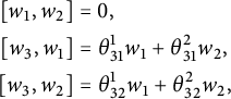 $$ \begin{align*} \left[w_1,w_2\right]&=0,\\ \left[w_3,w_1\right]&=\theta_{31}^1w_1+\theta_{31}^2w_2,\\ \left[w_3,w_2\right]&=\theta_{32}^1w_1+\theta_{32}^2w_2, \end{align*} $$
with
 $ 0\neq \operatorname {\mathrm{tr}} \mathrm {ad}_{w_3}=\theta _{31}^1+\theta _{32}^2. $
The basis
$ 0\neq \operatorname {\mathrm{tr}} \mathrm {ad}_{w_3}=\theta _{31}^1+\theta _{32}^2. $
The basis
![]() of
of
 $ \mathfrak {g} $
is orthonormal with respect to
$ \mathfrak {g} $
is orthonormal with respect to
 $ g $
satisfying
$ g $
satisfying
 $ g(v_1,v_1)=g(v_2,v_2)=-g(v_3,v_3) $
. If we define
$ g(v_1,v_1)=g(v_2,v_2)=-g(v_3,v_3) $
. If we define
![]() and
and
![]() , where
, where
 $ \varepsilon _a=g(v_a,v_a) $
, then
$ \varepsilon _a=g(v_a,v_a) $
, then
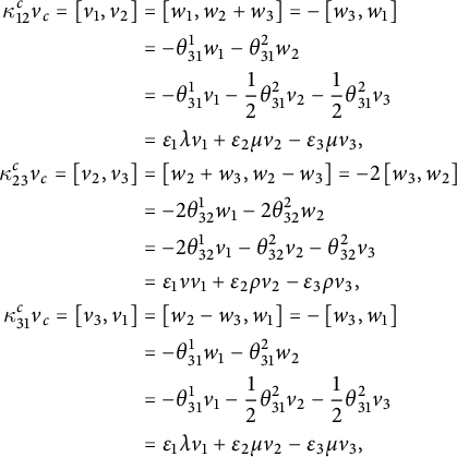 $$ \begin{align*} \kappa_{12}^cv_c=\left[v_1,v_2\right]&=\left[w_1,w_2+w_3\right]=-\left[w_3,w_1\right]\\ &=-\theta_{31}^1w_1-\theta_{31}^2w_2\\ &=-\theta_{31}^1v_1-\frac12\theta_{31}^2v_2-\frac12\theta_{31}^2v_3\\ &=\varepsilon_{1}\lambda v_1+\varepsilon_2\mu v_2-\varepsilon_3\mu v_3,\\ \kappa_{23}^cv_c=\left[v_2,v_3\right]&=\left[w_2+w_3,w_2-w_3\right]=-2\left[w_3,w_2\right]\\ &=-2\theta_{32}^1w_1-2\theta_{32}^2w_2\\ &=-2\theta_{32}^1v_1-\theta_{32}^2v_2-\theta_{32}^2v_3\\ &=\varepsilon_{1}\nu v_1+\varepsilon_2\rho v_2-\varepsilon_3\rho v_3,\\ \kappa_{31}^cv_c=\left[v_3,v_1\right]&=\left[w_2-w_3,w_1\right]=-\left[w_3,w_1\right]\\ &=-\theta_{31}^1w_1-\theta_{31}^2w_2\\ &=-\theta_{31}^1v_1-\frac12\theta_{31}^2v_2-\frac12\theta_{31}^2v_3\\ &=\varepsilon_{1}\lambda v_1+\varepsilon_2\mu v_2-\varepsilon_3\mu v_3, \end{align*} $$
with
 $ \lambda +\rho \neq 0 $
. Hence, the structure constants
$ \lambda +\rho \neq 0 $
. Hence, the structure constants
 $ \kappa _{abc} $
of
$ \kappa _{abc} $
of
 $ \mathfrak {g} $
with respect to
$ \mathfrak {g} $
with respect to
 $ (v_a)_a $
are
$ (v_a)_a $
are
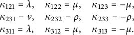 $$\begin{align*}\begin{array}{lll} \kappa_{121}=\lambda,&\kappa_{122}=\mu,&\kappa_{123}=-\mu,\\ \kappa_{231}=\nu,&\kappa_{232}=\rho,&\kappa_{233}=-\rho,\\ \kappa_{311}=\lambda,&\kappa_{312}=\mu,&\kappa_{313}=-\mu.\end{array} \end{align*}$$
Now, the Dorfman coefficients are
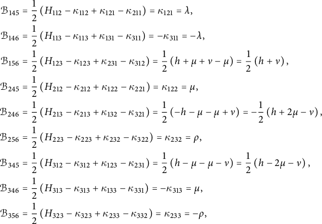 $$ \begin{align*} \mathcal B_{145}&=\frac12\left(H_{112}-\kappa_{112}+\kappa_{121}-\kappa_{211}\right)=\kappa_{121}=\lambda,\\ \mathcal B_{146}&=\frac12\left(H_{113}-\kappa_{113}+\kappa_{131}-\kappa_{311}\right)=-\kappa_{311}=-\lambda,\\ \mathcal B_{156}&=\frac12\left(H_{123}-\kappa_{123}+\kappa_{231}-\kappa_{312}\right)=\frac12\left(h+\mu+\nu-\mu\right)=\frac12\left(h+\nu\right),\\ \mathcal B_{245}&=\frac12\left(H_{212}-\kappa_{212}+\kappa_{122}-\kappa_{221}\right)=\kappa_{122}=\mu,\\ \mathcal B_{246}&=\frac12\left(H_{213}-\kappa_{213}+\kappa_{132}-\kappa_{321}\right)=\frac12\left(-h-\mu-\mu+\nu\right)=-\frac12\left(h+2\mu-\nu\right),\\ \mathcal B_{256}&=\frac12\left(H_{223}-\kappa_{223}+\kappa_{232}-\kappa_{322}\right)=\kappa_{232}=\rho,\\ \mathcal B_{345}&=\frac12\left(H_{312}-\kappa_{312}+\kappa_{123}-\kappa_{231}\right)=\frac12\left(h-\mu-\mu-\nu\right)=\frac12\left(h-2\mu-\nu\right),\\ \mathcal B_{346}&=\frac12\left(H_{313}-\kappa_{313}+\kappa_{133}-\kappa_{331}\right)=-\kappa_{313}=\mu,\\ \mathcal B_{356}&=\frac12\left(H_{323}-\kappa_{323}+\kappa_{233}-\kappa_{332}\right)=\kappa_{233}=-\rho, \end{align*} $$
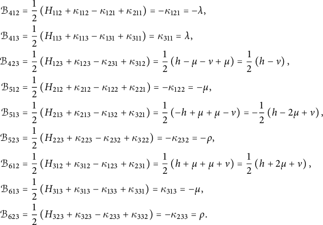 $$ \begin{align*} \mathcal B_{412}&=\frac12\left(H_{112}+\kappa_{112}-\kappa_{121}+\kappa_{211}\right)=-\kappa_{121}=-\lambda,\\ \mathcal B_{413}&=\frac12\left(H_{113}+\kappa_{113}-\kappa_{131}+\kappa_{311}\right)=\kappa_{311}=\lambda,\\ \mathcal B_{423}&=\frac12\left(H_{123}+\kappa_{123}-\kappa_{231}+\kappa_{312}\right)=\frac12\left(h-\mu-\nu+\mu\right)=\frac12\left(h-\nu\right),\\ \mathcal B_{512}&=\frac12\left(H_{212}+\kappa_{212}-\kappa_{122}+\kappa_{221}\right)=-\kappa_{122}=-\mu,\\ \mathcal B_{513}&=\frac12\left(H_{213}+\kappa_{213}-\kappa_{132}+\kappa_{321}\right)=\frac12\left(-h+\mu+\mu-\nu\right)=-\frac12\left(h-2\mu+\nu\right),\\ \mathcal B_{523}&=\frac12\left(H_{223}+\kappa_{223}-\kappa_{232}+\kappa_{322}\right)=-\kappa_{232}=-\rho,\\ \mathcal B_{612}&=\frac12\left(H_{312}+\kappa_{312}-\kappa_{123}+\kappa_{231}\right)=\frac12\left(h+\mu+\mu+\nu\right)=\frac12\left(h+2\mu+\nu\right),\\ \mathcal B_{613}&=\frac12\left(H_{313}+\kappa_{313}-\kappa_{133}+\kappa_{331}\right)=\kappa_{313}=-\mu,\\ \mathcal B_{623}&=\frac12\left(H_{323}+\kappa_{323}-\kappa_{233}+\kappa_{332}\right)=-\kappa_{233}=\rho. \end{align*} $$
By equation (26), the components of the generalized Ricci curvature are
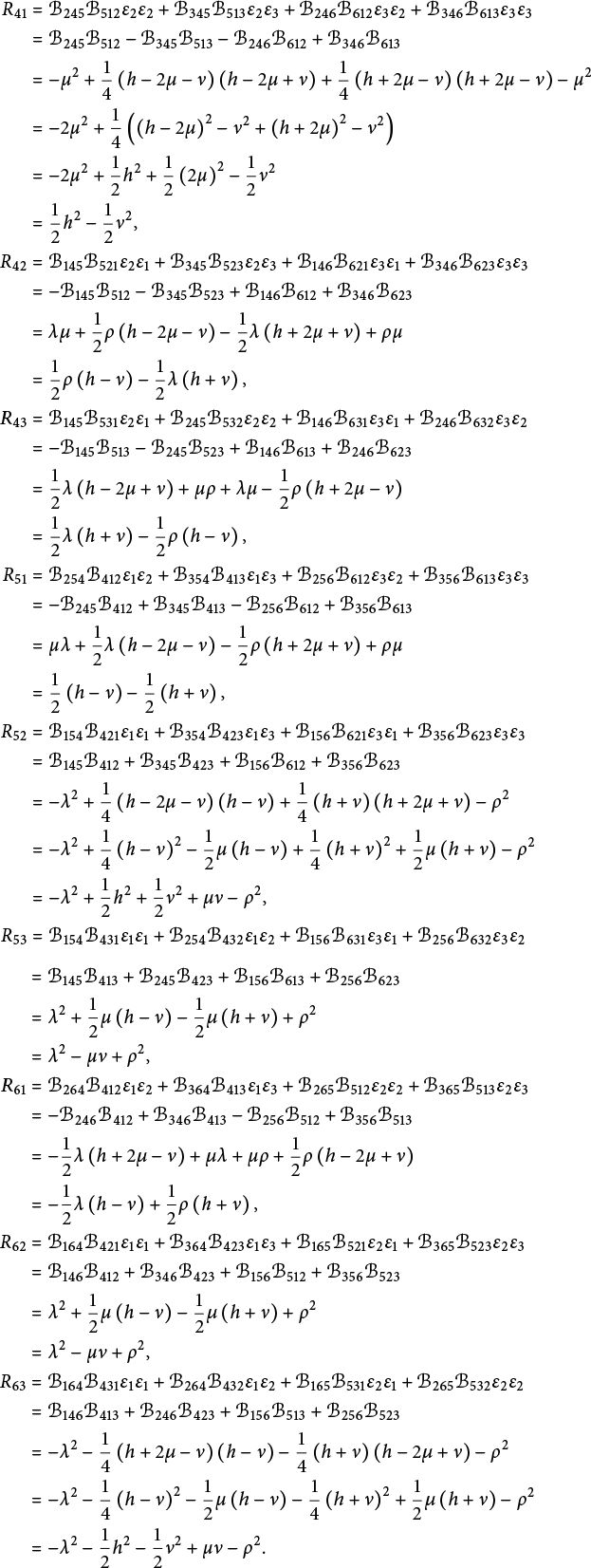 $$ \begin{align*} R_{41}&=\mathcal{B}_{245}\mathcal{B}_{512}\varepsilon_{2}\varepsilon_2+\mathcal{B}_{345}\mathcal{B}_{513}\varepsilon_{2}\varepsilon_3+\mathcal{B}_{246}\mathcal{B}_{612}\varepsilon_{3}\varepsilon_2+\mathcal{B}_{346}\mathcal{B}_{613}\varepsilon_{3}\varepsilon_3\\ &=\mathcal{B}_{245}\mathcal{B}_{512}-\mathcal{B}_{345}\mathcal{B}_{513}-\mathcal{B}_{246}\mathcal{B}_{612}+\mathcal{B}_{346}\mathcal{B}_{613}\\ &=-\mu^2+\frac14\left(h-2\mu-\nu\right)\left(h-2\mu+\nu\right)+\frac14\left(h+2\mu-\nu\right)\left(h+2\mu-\nu\right)-\mu^2\\ &=-2\mu^2+\frac14\left(\left(h-2\mu\right)^2-\nu^2+\left(h+2\mu\right)^2-\nu^2\right)\\ &=-2\mu^2+\frac12h^2+\frac12\left(2\mu\right)^2-\frac12\nu^2\\ &=\frac12h^2-\frac12\nu^2,\\ R_{42}&=\mathcal{B}_{145}\mathcal{B}_{521}\varepsilon_{2}\varepsilon_1+\mathcal{B}_{345}\mathcal{B}_{523}\varepsilon_{2}\varepsilon_3+\mathcal{B}_{146}\mathcal{B}_{621}\varepsilon_{3}\varepsilon_1+\mathcal{B}_{346}\mathcal{B}_{623}\varepsilon_{3}\varepsilon_3\\ &=-\mathcal{B}_{145}\mathcal{B}_{512}-\mathcal{B}_{345}\mathcal{B}_{523}+\mathcal{B}_{146}\mathcal{B}_{612}+\mathcal{B}_{346}\mathcal{B}_{623}\\ &=\lambda\mu+\frac12\rho\left(h-2\mu-\nu\right)-\frac12\lambda\left(h+2\mu+\nu\right)+\rho\mu\\ &=\frac12\rho\left(h-\nu\right)-\frac12\lambda\left(h+\nu\right),\\ R_{43}&=\mathcal{B}_{145}\mathcal{B}_{531}\varepsilon_{2}\varepsilon_1+\mathcal{B}_{245}\mathcal{B}_{532}\varepsilon_{2}\varepsilon_2+\mathcal{B}_{146}\mathcal{B}_{631}\varepsilon_{3}\varepsilon_1+\mathcal{B}_{246}\mathcal{B}_{632}\varepsilon_{3}\varepsilon_2\\ &=-\mathcal{B}_{145}\mathcal{B}_{513}-\mathcal{B}_{245}\mathcal{B}_{523}+\mathcal{B}_{146}\mathcal{B}_{613}+\mathcal{B}_{246}\mathcal{B}_{623}\\ &=\frac12\lambda\left(h-2\mu+\nu\right)+\mu\rho+\lambda\mu-\frac12\rho\left(h+2\mu-\nu\right)\\ &=\frac12\lambda\left(h+\nu\right)-\frac12\rho\left(h-\nu\right),\\ R_{51}&=\mathcal{B}_{254}\mathcal{B}_{412}\varepsilon_{1}\varepsilon_2+\mathcal{B}_{354}\mathcal{B}_{413}\varepsilon_{1}\varepsilon_3+\mathcal{B}_{256}\mathcal{B}_{612}\varepsilon_{3}\varepsilon_2+\mathcal{B}_{356}\mathcal{B}_{613}\varepsilon_{3}\varepsilon_3\\ &=-\mathcal{B}_{245}\mathcal{B}_{412}+\mathcal{B}_{345}\mathcal{B}_{413}-\mathcal{B}_{256}\mathcal{B}_{612}+\mathcal{B}_{356}\mathcal{B}_{613}\\ &=\mu\lambda+\frac12\lambda\left(h-2\mu-\nu\right)-\frac12\rho\left(h+2\mu+\nu\right)+\rho\mu\\ &=\frac12\left(h-\nu\right)-\frac12\left(h+\nu\right),\\ R_{52}&=\mathcal{B}_{154}\mathcal{B}_{421}\varepsilon_{1}\varepsilon_1+\mathcal{B}_{354}\mathcal{B}_{423}\varepsilon_{1}\varepsilon_3+\mathcal{B}_{156}\mathcal{B}_{621}\varepsilon_{3}\varepsilon_1+\mathcal{B}_{356}\mathcal{B}_{623}\varepsilon_{3}\varepsilon_3\\ &=\mathcal{B}_{145}\mathcal{B}_{412}+\mathcal{B}_{345}\mathcal{B}_{423}+\mathcal{B}_{156}\mathcal{B}_{612}+\mathcal{B}_{356}\mathcal{B}_{623}\\ &=-\lambda^2+\frac14\left(h-2\mu-\nu\right)\left(h-\nu\right)+\frac14\left(h+\nu\right)\left(h+2\mu+\nu\right)-\rho^2\\ &=-\lambda^2+\frac14\left(h-\nu\right)^2-\frac12\mu\left(h-\nu\right)+\frac14\left(h+\nu\right)^2+\frac12\mu\left(h+\nu\right)-\rho^2\\ &=-\lambda^2+\frac12h^2+\frac12\nu^2+\mu\nu-\rho^2,\\ R_{53}&=\mathcal{B}_{154}\mathcal{B}_{431}\varepsilon_{1}\varepsilon_1+\mathcal{B}_{254}\mathcal{B}_{432}\varepsilon_{1}\varepsilon_2+\mathcal{B}_{156}\mathcal{B}_{631}\varepsilon_{3}\varepsilon_1+\mathcal{B}_{256}\mathcal{B}_{632}\varepsilon_{3}\varepsilon_2\\ &=\mathcal{B}_{145}\mathcal{B}_{413}+\mathcal{B}_{245}\mathcal{B}_{423}+\mathcal{B}_{156}\mathcal{B}_{613}+\mathcal{B}_{256}\mathcal{B}_{623}\\ &=\lambda^2+\frac12\mu\left(h-\nu\right)-\frac12\mu\left(h+\nu\right)+\rho^2\\ &=\lambda^2-\mu\nu+\rho^2,\\ R_{61}&=\mathcal{B}_{264}\mathcal{B}_{412}\varepsilon_{1}\varepsilon_2+\mathcal{B}_{364}\mathcal{B}_{413}\varepsilon_{1}\varepsilon_3+\mathcal{B}_{265}\mathcal{B}_{512}\varepsilon_{2}\varepsilon_2+\mathcal{B}_{365}\mathcal{B}_{513}\varepsilon_{2}\varepsilon_3\\ &=-\mathcal{B}_{246}\mathcal{B}_{412}+\mathcal{B}_{346}\mathcal{B}_{413}-\mathcal{B}_{256}\mathcal{B}_{512}+\mathcal{B}_{356}\mathcal{B}_{513}\\ &=-\frac12\lambda\left(h+2\mu-\nu\right)+\mu\lambda+\mu\rho+\frac12\rho\left(h-2\mu+\nu\right)\\ &=-\frac12\lambda\left(h-\nu\right)+\frac12\rho\left(h+\nu\right),\\ R_{62}&=\mathcal{B}_{164}\mathcal{B}_{421}\varepsilon_{1}\varepsilon_1+\mathcal{B}_{364}\mathcal{B}_{423}\varepsilon_{1}\varepsilon_3+\mathcal{B}_{165}\mathcal{B}_{521}\varepsilon_{2}\varepsilon_1+\mathcal{B}_{365}\mathcal{B}_{523}\varepsilon_{2}\varepsilon_3\\ &=\mathcal{B}_{146}\mathcal{B}_{412}+\mathcal{B}_{346}\mathcal{B}_{423}+\mathcal{B}_{156}\mathcal{B}_{512}+\mathcal{B}_{356}\mathcal{B}_{523}\\ &=\lambda^2+\frac12\mu\left(h-\nu\right)-\frac12\mu\left(h+\nu\right)+\rho^2\\ &=\lambda^2-\mu\nu+\rho^2,\\ R_{63}&=\mathcal{B}_{164}\mathcal{B}_{431}\varepsilon_{1}\varepsilon_1+\mathcal{B}_{264}\mathcal{B}_{432}\varepsilon_{1}\varepsilon_2+\mathcal{B}_{165}\mathcal{B}_{531}\varepsilon_{2}\varepsilon_1+\mathcal{B}_{265}\mathcal{B}_{532}\varepsilon_{2}\varepsilon_2\\ &=\mathcal{B}_{146}\mathcal{B}_{413}+\mathcal{B}_{246}\mathcal{B}_{423}+\mathcal{B}_{156}\mathcal{B}_{513}+\mathcal{B}_{256}\mathcal{B}_{523}\\ &=-\lambda^2-\frac14\left(h+2\mu-\nu\right)\left(h-\nu\right)-\frac14\left(h+\nu\right)\left(h-2\mu+\nu\right)-\rho^2\\ &=-\lambda^2-\frac14\left(h-\nu\right)^2-\frac12\mu\left(h-\nu\right)-\frac14\left(h+\nu\right)^2+\frac12\mu\left(h+\nu\right)-\rho^2\\ &=-\lambda^2-\frac12h^2-\frac12\nu^2+\mu\nu-\rho^2. \end{align*} $$
If we impose the Einstein condition, we see that
 $ 0=R_{52}-R_{63}=h^2+\nu ^2 $
, hence
$ 0=R_{52}-R_{63}=h^2+\nu ^2 $
, hence
 $ h=\nu =0 $
. Therefore, the equation
$ h=\nu =0 $
. Therefore, the equation
 $ R_{63}=0 $
reads as
$ R_{63}=0 $
reads as
 $ 0=-\lambda ^2-\rho ^2 $
. This implies
$ 0=-\lambda ^2-\rho ^2 $
. This implies
 $ \lambda =\rho =0 $
, which is a contradiction to
$ \lambda =\rho =0 $
, which is a contradiction to
 $ \lambda +\rho \neq 0 $
.
$ \lambda +\rho \neq 0 $
.
We summarize this by the following theorem.
Theorem 3.8 Let
 $(H,\mathcal G_g,\delta =0)$
be a divergence-free generalized Einstein structure on a three-dimensional nonunimodular Lie group G. Then
$(H,\mathcal G_g,\delta =0)$
be a divergence-free generalized Einstein structure on a three-dimensional nonunimodular Lie group G. Then
 $ H=0 $
and
$ H=0 $
and
 $ g $
is indefinite. Furthermore, there exists an orthonormal basis
$ g $
is indefinite. Furthermore, there exists an orthonormal basis
 $(v_a)$
of
$(v_a)$
of
 $(\mathfrak {g},g)$
such that
$(\mathfrak {g},g)$
such that
 $ v_1,v_3\in \mathfrak {u} $
and
$ v_1,v_3\in \mathfrak {u} $
and
 $g(v_1,v_1)=g(v_2,v_2)=-g(v_3,v_3)$
as well as a positive constant
$g(v_1,v_1)=g(v_2,v_2)=-g(v_3,v_3)$
as well as a positive constant
 $\theta>0$
such that
$\theta>0$
such that
 $$ \begin{align*} [v_1,v_3]&=0,\\ \left[v_2,v_1\right]&=\theta v_1-\theta v_3,\\ \left[v_2,v_3\right]&=\theta v_1+\theta v_3. \end{align*} $$
The metric g is a Ricci soliton which is not of constant curvature.
Proof It remains to prove the last statement. The fact that g is a Ricci soliton is a direct consequence of Corollary 2.30. To see that the metric is nonflat, it suffices to check that
 $\nabla \tau \neq 0$
. Since
$\nabla \tau \neq 0$
. Since
 $\tau = 2\theta v_2^*$
, where
$\tau = 2\theta v_2^*$
, where
 $(v_a^*)$
denotes the dual basis, it suffices to compute
$(v_a^*)$
denotes the dual basis, it suffices to compute
 $\nabla v_2$
:
$\nabla v_2$
:
 $$\begin{align*}g(\nabla_{v_1}v_2,v_1) = g([v_1,v_2],v_1) = -\theta \varepsilon_1\neq 0.\\[-15pt]\end{align*}$$
Similarly,
 $\nabla _{v_2}v_2=0$
shows that g is neither of nonzero constant curvature.
$\nabla _{v_2}v_2=0$
shows that g is neither of nonzero constant curvature.
Corollary 3.9 If the metric is definite, there are no solutions to the Ricci soliton equation ( 22 ) in the nonunimodular case.
Remark 3.10 Note that in all our proofs in the unimodular and in the nonunimodular case, we only used that the diagonal components
 $ R_{ii'} $
are zero. In particular, the Ricci tensor is zero, if
$ R_{ii'} $
are zero. In particular, the Ricci tensor is zero, if
 $ R_{ii'}=0 $
for all
$ R_{ii'}=0 $
for all
 $ i\in \{4,5,6\} $
, in the divergence free case.
$ i\in \{4,5,6\} $
, in the divergence free case.
3.3 Arbitrary divergence
Recall that
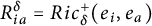 $R_{ia}^{\delta }=Ric^+_{\delta } (e_i,e_a)$
and
$R_{ia}^{\delta }=Ric^+_{\delta } (e_i,e_a)$
and
 $R_{ai}^{\delta }=Ric^-_{\delta } (e_a,e_i)$
denote the components of the Ricci curvature tensors
$R_{ai}^{\delta }=Ric^-_{\delta } (e_a,e_i)$
denote the components of the Ricci curvature tensors
 $Ric^{\pm }_{\delta }$
of a generalized pseudo-Riemannian Lie group
$Ric^{\pm }_{\delta }$
of a generalized pseudo-Riemannian Lie group
 $(G,H,\mathcal G_g,\delta )$
with arbitrary divergence
$(G,H,\mathcal G_g,\delta )$
with arbitrary divergence
 $\delta \in E^*$
. If
$\delta \in E^*$
. If
 $ \delta =0 $
we often write
$ \delta =0 $
we often write
 $ R_{ia}=R_{ia}^0 $
and
$ R_{ia}=R_{ia}^0 $
and
 $ R_{ai}=R_{ai}^0 $
. By Theorem 2.25, we have
$ R_{ai}=R_{ai}^0 $
. By Theorem 2.25, we have
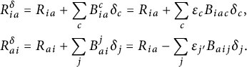 $$ \begin{align*} R_{ia}^{\delta}&=R_{ia}+\sum_cB_{ia}^c\delta_c=R_{ia}+\sum_c\varepsilon_cB_{iac}\delta_c,\\ R_{ai}^{\delta}&=R_{ai}+\sum_jB_{ai}^j\delta_j=R_{ia}-\sum_{j}\varepsilon_{j'}B_{aij}\delta_j.\\[-15pt] \end{align*} $$
3.3.1 Unimodular Lie groups
Proposition 3.11 If
 $(H,\mathcal G_g,\delta )$
is a generalized Einstein structure on an oriented three-dimensional unimodular Lie group G, then there exists a
$(H,\mathcal G_g,\delta )$
is a generalized Einstein structure on an oriented three-dimensional unimodular Lie group G, then there exists a
 $ g $
-orthonormal basis
$ g $
-orthonormal basis
 $(v_a)$
of
$(v_a)$
of
 $\mathfrak {g}$
such that
$\mathfrak {g}$
such that
 $g(v_1,v_1)=g(v_2,v_2)$
and such that the symmetric endomorphism L defined in equation (
23
) takes one of the following forms:
$g(v_1,v_1)=g(v_2,v_2)$
and such that the symmetric endomorphism L defined in equation (
23
) takes one of the following forms:
-
(1)
$ L_1(\alpha ,\beta ,\gamma ) $
, that is,
$ L $
is diagonalizable by an orthonormal basis. -
(2)
$ L_3(\alpha ,0) $
or
$ L_4(\alpha ,0) $
, in both cases
$ -\varepsilon _1\frac 12\delta _1=-\varepsilon _1\frac 12\delta _4=\alpha $
as well as
$ \delta _2=\delta _3 $
and
$ \delta _5=\delta _6 $
. If
$ \alpha \ne 0 $
, then
$ \delta _2=\delta _3=\delta _5=\delta _6=0 $
. -
(3)
$ L_5(0) $
with
$ \delta _2=\delta _5=0 $
and
$ \delta _1=\delta _3=\delta _4=\delta _6=-\varepsilon _1\sqrt 2 $
, where
$ \delta _a=\delta (v_a+g(v_a)) $
and
$ \delta _i=\delta (v_{i'}-g(v_{i'})) $
.


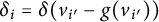
Furthermore, in the nondiagonalizable case, the three-form
 $ H $
is always zero (see Proposition 3.2 for the notation of the normal forms of
$ H $
is always zero (see Proposition 3.2 for the notation of the normal forms of
 $ L $
).
$ L $
).
Proof Since in the Euclidean case, any symmetric endomorphism is always diagonalizable by an orthonormal basis, we may assume that the scalar product is indefinite. By Proposition 3.2, there is an orthonormal basis
 $ (v_a) $
, such that the endomorphism
$ (v_a) $
, such that the endomorphism
 $ L $
takes one of the normal forms
$ L $
takes one of the normal forms
 $L_1(\alpha , \beta , \gamma ), L_2(\alpha , \beta , \gamma ), L_3(\alpha , \beta ), L_4(\alpha , \beta ),$
or
$L_1(\alpha , \beta , \gamma ), L_2(\alpha , \beta , \gamma ), L_3(\alpha , \beta ), L_4(\alpha , \beta ),$
or
 $L_5(\alpha )$
from said proposition. As in the proof of Proposition 3.3, we can treat all these cases at once by considering the matrix
$L_5(\alpha )$
from said proposition. As in the proof of Proposition 3.3, we can treat all these cases at once by considering the matrix
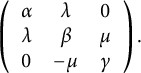 $$\begin{align*}\left(\begin{array}{ccc}\alpha &\lambda &0\\ \lambda &\beta &\mu \\ 0&-\mu&\gamma\end{array} \right). \end{align*}$$
Recall that we assume
 $ \varepsilon _{1}=\varepsilon _2=-\varepsilon _{3} $
, where
$ \varepsilon _{1}=\varepsilon _2=-\varepsilon _{3} $
, where
 $ \varepsilon _a=g(v_a,v_a) $
. Using the Dorfman coefficients and the coefficients of the Ricci curvature with divergence zero from the proof of Proposition 3.3, we can compute the components of the Ricci curvature with divergence
$ \varepsilon _a=g(v_a,v_a) $
. Using the Dorfman coefficients and the coefficients of the Ricci curvature with divergence zero from the proof of Proposition 3.3, we can compute the components of the Ricci curvature with divergence
 $ \delta $
as
$ \delta $
as
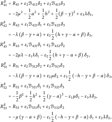 $$ \begin{align*} R_{41}^{\delta}&=R_{41}+\varepsilon_2\mathcal{B}_{412}\delta_2+\varepsilon_3\mathcal{B}_{413}\delta_3\\ &=-2\mu^2-\frac12\alpha^2+\frac12h^2+\frac12(\beta-\gamma)^2+\varepsilon_3\lambda\delta_3,\\ R_{42}^{\delta}&=R_{42}+\varepsilon_1\mathcal{B}_{421}\delta_1+\varepsilon_3\mathcal{B}_{423}\delta_3\\ &=-\lambda\left(\beta-\gamma+\alpha\right)+\varepsilon_3\frac12\left(h+\gamma-\alpha+\beta\right)\delta_3,\\ R_{43}^{\delta}&=R_{43}+\varepsilon_1\mathcal{B}_{431}\delta_1+\varepsilon_2\mathcal{B}_{432}\delta_2\\ &=-2\mu\lambda-\varepsilon_{1}\lambda\delta_1-\varepsilon_{2}\frac12\left(h+\gamma-\alpha+\beta\right)\delta_2,\\ R_{51}^{\delta}&=R_{51}+\varepsilon_2\mathcal{B}_{512}\delta_2+\varepsilon_3\mathcal{B}_{513}\delta_3\\ &=-\lambda\left(\beta-\gamma+\alpha\right)+\varepsilon_{2}\mu\delta_2+\varepsilon_{3}\frac12\left(-h-\gamma+\beta-\alpha\right)\delta_3,\\ R_{52}^{\delta}&=R_{52}+\varepsilon_1\mathcal{B}_{521}\delta_1+\varepsilon_3\mathcal{B}_{523}\delta_3\\ &=-\frac12\beta^2+\frac12h^2+\frac12\left(\gamma-\alpha\right)^2-\varepsilon_{1}\mu\delta_1-\varepsilon_{3}\lambda\delta_3,\\ R_{53}^{\delta}&=R_{53}+\varepsilon_1\mathcal{B}_{531}\delta_1+\varepsilon_2\mathcal{B}_{532}\delta_2\\ &=-\mu\left(\gamma-\alpha+\beta\right)-\varepsilon_1\frac12\left(-h-\gamma+\beta-\alpha\right)\delta_1+\varepsilon_{2}\lambda\delta_2, \end{align*} $$
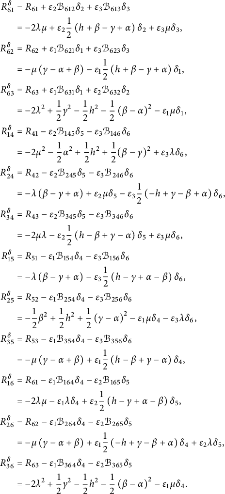 $$ \begin{align*} R_{61}^{\delta}&=R_{61}+\varepsilon_2\mathcal{B}_{612}\delta_2+\varepsilon_3\mathcal{B}_{613}\delta_3\\ &=-2\lambda\mu+\varepsilon_{2}\frac12\left(h+\beta-\gamma+\alpha\right)\delta_2+\varepsilon_3\mu\delta_3,\\ R_{62}^{\delta}&=R_{62}+\varepsilon_1\mathcal{B}_{621}\delta_1+\varepsilon_3\mathcal{B}_{623}\delta_3\\ &=-\mu\left(\gamma-\alpha+\beta\right)-\varepsilon_1\frac12\left(h+\beta-\gamma+\alpha\right)\delta_1,\\ R_{63}^{\delta}&=R_{63}+\varepsilon_1\mathcal{B}_{631}\delta_1+\varepsilon_2\mathcal{B}_{632}\delta_2\\ &=-2\lambda^2+\frac12\gamma^2-\frac12h^2-\frac12\left(\beta-\alpha\right)^2-\varepsilon_{1}\mu\delta_1,\\ R_{14}^{\delta}&=R_{41}-\varepsilon_2\mathcal{B}_{145}\delta_5-\varepsilon_3\mathcal{B}_{146}\delta_6\\ &=-2\mu^2-\frac12\alpha^2+\frac12h^2+\frac12(\beta-\gamma)^2+\varepsilon_3\lambda\delta_6,\\ R_{24}^{\delta}&=R_{42}-\varepsilon_2\mathcal{B}_{245}\delta_5-\varepsilon_3\mathcal{B}_{246}\delta_6\\ &=-\lambda\left(\beta-\gamma+\alpha\right)+\varepsilon_2\mu\delta_5-\varepsilon_3\frac12\left(-h+\gamma-\beta+\alpha\right)\delta_6,\\ R_{34}^{\delta}&=R_{43}-\varepsilon_2\mathcal{B}_{345}\delta_5-\varepsilon_3\mathcal{B}_{346}\delta_6\\ &=-2\mu\lambda-\varepsilon_{2}\frac12\left(h-\beta+\gamma-\alpha\right)\delta_5+\varepsilon_{3}\mu\delta_6,\\ R_{15}^{\delta}&=R_{51}-\varepsilon_1\mathcal{B}_{154}\delta_4-\varepsilon_3\mathcal{B}_{156}\delta_6\\ &=-\lambda\left(\beta-\gamma+\alpha\right)-\varepsilon_{3}\frac12\left(h-\gamma+\alpha-\beta\right)\delta_6,\\ R_{25}^{\delta}&=R_{52}-\varepsilon_1\mathcal{B}_{254}\delta_4-\varepsilon_3\mathcal{B}_{256}\delta_6\\ &=-\frac12\beta^2+\frac12h^2+\frac12\left(\gamma-\alpha\right)^2-\varepsilon_{1}\mu\delta_4-\varepsilon_3\lambda\delta_6,\\ R_{35}^{\delta}&=R_{53}-\varepsilon_1\mathcal{B}_{354}\delta_4-\varepsilon_3\mathcal{B}_{356}\delta_6\\ &=-\mu\left(\gamma-\alpha+\beta\right)+\varepsilon_{1}\frac12\left(h-\beta+\gamma-\alpha\right)\delta_4,\\ R_{16}^{\delta}&=R_{61}-\varepsilon_1\mathcal{B}_{164}\delta_4-\varepsilon_2\mathcal{B}_{165}\delta_5\\ &=-2\lambda\mu-\varepsilon_{1}\lambda\delta_4+\varepsilon_2\frac12\left(h-\gamma+\alpha-\beta\right)\delta_5,\\ R_{26}^{\delta}&=R_{62}-\varepsilon_1\mathcal{B}_{264}\delta_4-\varepsilon_2\mathcal{B}_{265}\delta_5\\ &=-\mu\left(\gamma-\alpha+\beta\right)+\varepsilon_1\frac12\left(-h+\gamma-\beta+\alpha\right)\delta_4+\varepsilon_2\lambda\delta_5,\\ R_{36}^{\delta}&=R_{63}-\varepsilon_1\mathcal{B}_{364}\delta_4-\varepsilon_2\mathcal{B}_{365}\delta_5\\ &=-2\lambda^2+\frac12\gamma^2-\frac12h^2-\frac12\left(\beta-\alpha\right)^2-\varepsilon_{1}\mu\delta_4. \end{align*} $$
For the normal form
 $ L_2(\alpha ,\beta ,\gamma ), $
the equations for
$ L_2(\alpha ,\beta ,\gamma ), $
the equations for
 $ Ric^+_{\delta } $
read
$ Ric^+_{\delta } $
read
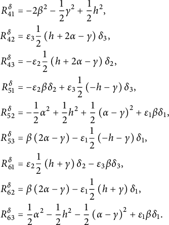 $$ \begin{align*} R_{41}^{\delta}&=-2\beta^2-\frac12\gamma^2+\frac12h^2,\\ R_{42}^{\delta}&=\varepsilon_3\frac12\left(h+2\alpha-\gamma\right)\delta_3,\\ R_{43}^{\delta}&=-\varepsilon_2\frac12\left(h+2\alpha-\gamma\right)\delta_2,\\ R_{51}^{\delta}&=-\varepsilon_2\beta\delta_2+\varepsilon_3\frac12\left(-h-\gamma\right)\delta_3,\\ R_{52}^{\delta}&=-\frac12\alpha^2+\frac12h^2+\frac12\left(\alpha-\gamma\right)^2+\varepsilon_1\beta\delta_1,\\ R_{53}^{\delta}&=\beta\left(2\alpha-\gamma\right)-\varepsilon_{1}\frac12\left(-h-\gamma\right)\delta_1,\\ R_{61}^{\delta}&=\varepsilon_2\frac12\left(h+\gamma\right)\delta_2-\varepsilon_3\beta\delta_3,\\ R_{62}^{\delta}&=\beta\left(2\alpha-\gamma\right)-\varepsilon_1\frac12\left(h+\gamma\right)\delta_1,\\ R_{63}^{\delta}&=\frac12\alpha^2-\frac12h^2-\frac12\left(\alpha-\gamma\right)^2+\varepsilon_1\beta\delta_1. \end{align*} $$
Imposing now the Einstein condition, we get
 $ 0=R_{53}^{\delta }+R_{62}^{\delta }=2\beta \left (2\alpha -\gamma \right ) $
. So either
$ 0=R_{53}^{\delta }+R_{62}^{\delta }=2\beta \left (2\alpha -\gamma \right ) $
. So either
 $ L $
is diagonalizable, if
$ L $
is diagonalizable, if
 $ \beta =0 $
, or
$ \beta =0 $
, or
 $ 2\alpha =\gamma $
. But then, the equation
$ 2\alpha =\gamma $
. But then, the equation
 $ 0=R_{52}^{\delta }-R_{63}^{\delta } $
is
$ 0=R_{52}^{\delta }-R_{63}^{\delta } $
is
 $$\begin{align*}0=-\alpha^2+h^2+\left(\alpha-\gamma\right)^2=h^2, \end{align*}$$
and hence
 $ h=0 $
. Applying this to the equation for
$ h=0 $
. Applying this to the equation for
 $ R_{41}^{\delta } $
yields
$ R_{41}^{\delta } $
yields
 $ 0=-2\beta ^2-\frac 12\gamma ^2 $
. Therefore,
$ 0=-2\beta ^2-\frac 12\gamma ^2 $
. Therefore,
 $ \beta =0 $
and the endomorphism
$ \beta =0 $
and the endomorphism
 $ L $
is diagonalizable by an orthonormal basis.
$ L $
is diagonalizable by an orthonormal basis.
If
 $ L $
takes the normal form
$ L $
takes the normal form
 $ L_3(\alpha ,\beta ) $
, the components of the Ricci tensor are
$ L_3(\alpha ,\beta ) $
, the components of the Ricci tensor are
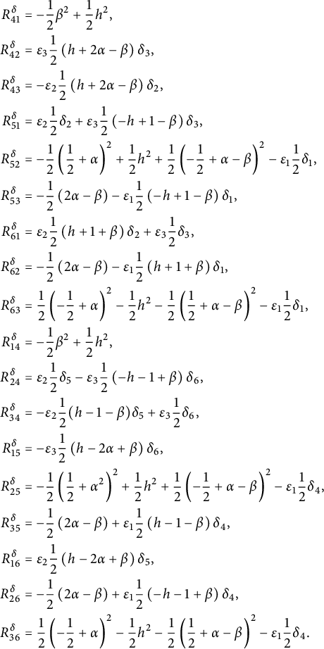 $$ \begin{align*} R_{41}^{\delta}&=-\frac12\beta^2+\frac12h^2,\\ R_{42}^{\delta}&=\varepsilon_3\frac12\left(h+2\alpha-\beta\right)\delta_3,\\ R_{43}^{\delta}&=-\varepsilon_2\frac12\left(h+2\alpha-\beta\right)\delta_2,\\ R_{51}^{\delta}&=\varepsilon_{2}\frac12\delta_2+\varepsilon_3\frac12\left(-h+1-\beta\right)\delta_3,\\ R_{52}^{\delta}&=-\frac12\left(\frac12+\alpha\right)^2+\frac12h^2+\frac12\left(-\frac12+\alpha-\beta\right)^2-\varepsilon_1\frac12\delta_1,\\ R_{53}^{\delta}&=-\frac12\left(2\alpha-\beta\right)-\varepsilon_{1}\frac12\left(-h+1-\beta\right)\delta_1,\\ R_{61}^{\delta}&=\varepsilon_2\frac12\left(h+1+\beta\right)\delta_2+\varepsilon_3\frac12\delta_3,\\ R_{62}^{\delta}&=-\frac12\left(2\alpha-\beta\right)-\varepsilon_1\frac12\left(h+1+\beta\right)\delta_1,\\ R_{63}^{\delta}&=\frac12\left(-\frac12+\alpha\right)^2-\frac12h^2-\frac12\left(\frac12+\alpha-\beta\right)^2-\varepsilon_1\frac12\delta_1,\\ R_{14}^{\delta}&=-\frac12\beta^2+\frac12h^2,\\ R_{24}^{\delta}&=\varepsilon_2\frac12\delta_5-\varepsilon_3\frac12\left(-h-1+\beta\right)\delta_6,\\ R_{34}^{\delta}&=-\varepsilon_2\frac12(h-1-\beta)\delta_5+\varepsilon_3\frac12\delta_6,\\ R_{15}^{\delta}&=-\varepsilon_3\frac12\left(h-2\alpha+\beta\right)\delta_6,\\ R_{25}^{\delta}&=-\frac12\left(\frac12+\alpha^2\right)^2+\frac12h^2+\frac12\left(-\frac12+\alpha-\beta\right)^2-\varepsilon_1\frac12\delta_4,\\ R_{35}^{\delta}&=-\frac12\left(2\alpha-\beta\right)+\varepsilon_1\frac12\left(h-1-\beta\right)\delta_4,\\ R_{16}^{\delta}&=\varepsilon_2\frac12\left(h-2\alpha+\beta\right)\delta_5,\\ R_{26}^{\delta}&=-\frac12\left(2\alpha-\beta\right)+\varepsilon_1\frac12\left(-h-1+\beta\right)\delta_4,\\ R_{36}^{\delta}&=\frac12\left(-\frac12+\alpha\right)^2-\frac12h^2-\frac12\left(\frac12+\alpha-\beta\right)^2-\varepsilon_1\frac12\delta_4. \end{align*} $$
First, equation
 $ R_{63}^{\delta }-R_{36}^{\delta }=0 $
yields
$ R_{63}^{\delta }-R_{36}^{\delta }=0 $
yields
 $ \delta _1=\delta _4 $
. Furthermore, due to
$ \delta _1=\delta _4 $
. Furthermore, due to
 $ 0=R_{53}^{\delta }-R_{62}^{\delta }=\varepsilon _1\left (h+\beta \right )\delta _1 $
and
$ 0=R_{53}^{\delta }-R_{62}^{\delta }=\varepsilon _1\left (h+\beta \right )\delta _1 $
and
 $ 0=R_{35}^{\delta }-R_{26}^{\delta }=\varepsilon _1\left (h-\beta \right )\delta _4=\varepsilon _1\left (h-\beta \right )\delta _1 $
, we have
$ 0=R_{35}^{\delta }-R_{26}^{\delta }=\varepsilon _1\left (h-\beta \right )\delta _4=\varepsilon _1\left (h-\beta \right )\delta _1 $
, we have
 $ \varepsilon _1\beta \delta _1=0 $
. If
$ \varepsilon _1\beta \delta _1=0 $
. If
 $ \delta _1=0 $
, then we see from
$ \delta _1=0 $
, then we see from
 $ 0=R_{53}^{\delta }=-\frac 12\left (2\alpha -\beta \right ) $
that
$ 0=R_{53}^{\delta }=-\frac 12\left (2\alpha -\beta \right ) $
that
 $ 2\alpha =\beta $
. Then
$ 2\alpha =\beta $
. Then
 $ 0=R_{63}^{\delta }=\frac 12\left (-\frac 12+\alpha \right )^2-\frac 12h^2-\frac 12\left (\frac 12-\alpha \right )^2=-\frac 12h^2 $
and
$ 0=R_{63}^{\delta }=\frac 12\left (-\frac 12+\alpha \right )^2-\frac 12h^2-\frac 12\left (\frac 12-\alpha \right )^2=-\frac 12h^2 $
and
 $ h=0 $
. Equation
$ h=0 $
. Equation
 $ R_{41}^{\delta }=0 $
shows
$ R_{41}^{\delta }=0 $
shows
 $ \beta =0 $
and therefore
$ \beta =0 $
and therefore
 $ \alpha =0 $
. Furthermore,
$ \alpha =0 $
. Furthermore,
 $ R_{51}^{\delta }=0 $
shows
$ R_{51}^{\delta }=0 $
shows
 $ \delta _2=\delta _3 $
and
$ \delta _2=\delta _3 $
and
 $ R_{15}^{\delta }=0 $
shows
$ R_{15}^{\delta }=0 $
shows
 $ \delta _5=\delta _6 $
, because
$ \delta _5=\delta _6 $
, because
 $ \varepsilon _2=-\varepsilon _3 $
. If otherwise
$ \varepsilon _2=-\varepsilon _3 $
. If otherwise
 $ \beta =0 $
, we see again from
$ \beta =0 $
, we see again from
 $ R_{41}^{\delta }=0 $
that
$ R_{41}^{\delta }=0 $
that
 $ h=0 $
and also
$ h=0 $
and also
 $ \delta _2=\delta _3 $
and
$ \delta _2=\delta _3 $
and
 $ \delta _5=\delta _6 $
, because of
$ \delta _5=\delta _6 $
, because of
 $ R_{51}^{\delta }=0 $
and
$ R_{51}^{\delta }=0 $
and
 $ R_{15}^{\delta }=0 $
, respectively. Finally,
$ R_{15}^{\delta }=0 $
, respectively. Finally,
 $ 0=\alpha \delta _2=\alpha \delta _3=\alpha \delta _2=\alpha \delta _3 $
due to
$ 0=\alpha \delta _2=\alpha \delta _3=\alpha \delta _2=\alpha \delta _3 $
due to
 $ 0=R_{42}^{\delta }=R_{43}^{\delta }=R_{15}^{\delta }=R_{16}^{\delta } $
, as well as
$ 0=R_{42}^{\delta }=R_{43}^{\delta }=R_{15}^{\delta }=R_{16}^{\delta } $
, as well as
 $ \alpha =-\varepsilon _1\frac 12\delta _1=-\varepsilon _1\frac 12\delta _4 $
due to
$ \alpha =-\varepsilon _1\frac 12\delta _1=-\varepsilon _1\frac 12\delta _4 $
due to
 $ R_{62}^{\delta }=R_{26}^{\delta }=0 $
.
$ R_{62}^{\delta }=R_{26}^{\delta }=0 $
.
In a similar way, we obtain the same equations for the normal form
 $ L_4(\alpha , \beta ) $
.
$ L_4(\alpha , \beta ) $
.
Finally, the equations for
 $ Ric^+_{\delta } $
for the normal form
$ Ric^+_{\delta } $
for the normal form
 $ L_5(\alpha ) $
are
$ L_5(\alpha ) $
are
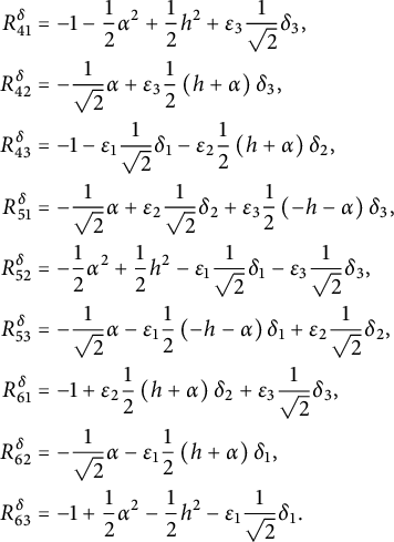 $$ \begin{align*} R_{41}^{\delta}&=-1-\frac12\alpha^2+\frac12h^2+\varepsilon_3\frac{1}{\sqrt2}\delta_3,\\ R_{42}^{\delta}&=-\frac{1}{\sqrt2}\alpha+\varepsilon_3\frac12\left(h+\alpha\right)\delta_3,\\ R_{43}^{\delta}&=-1-\varepsilon_1\frac{1}{\sqrt2}\delta_1-\varepsilon_2\frac12\left(h+\alpha\right)\delta_2,\\ R_{51}^{\delta}&=-\frac{1}{\sqrt2}\alpha+\varepsilon_2\frac{1}{\sqrt2}\delta_2+\varepsilon_3\frac12\left(-h-\alpha\right)\delta_3,\\ R_{52}^{\delta}&=-\frac12\alpha^2+\frac12h^2-\varepsilon_{1}\frac{1}{\sqrt2}\delta_1-\varepsilon_3\frac{1}{\sqrt2}\delta_3,\\ R_{53}^{\delta}&=-\frac{1}{\sqrt2}\alpha-\varepsilon_1\frac12\left(-h-\alpha\right)\delta_1+\varepsilon_2\frac{1}{\sqrt2}\delta_2,\\ R_{61}^{\delta}&=-1+\varepsilon_2\frac12\left(h+\alpha\right)\delta_2+\varepsilon_3\frac{1}{\sqrt2}\delta_3,\\ R_{62}^{\delta}&=-\frac{1}{\sqrt2}\alpha-\varepsilon_1\frac12\left(h+\alpha\right)\delta_1,\\ R_{63}^{\delta}&=-1+\frac12\alpha^2-\frac12h^2-\varepsilon_1\frac{1}{\sqrt2}\delta_1. \end{align*} $$
From
 $ 0=R_{41}^{\delta }-R_{52}^{\delta }-R_{63}^{\delta }=-\frac 12\left (\alpha ^2-h^2\right ), $
we see
$ 0=R_{41}^{\delta }-R_{52}^{\delta }-R_{63}^{\delta }=-\frac 12\left (\alpha ^2-h^2\right ), $
we see
 $ \alpha ^2=h^2 $
. Therefore,
$ \alpha ^2=h^2 $
. Therefore,
 $ \varepsilon _3\delta _3=\sqrt 2 $
by
$ \varepsilon _3\delta _3=\sqrt 2 $
by
 $ 0=R_{41}^{\delta }=-1+\varepsilon _3\frac {1}{\sqrt 2}\delta _3 $
as well as
$ 0=R_{41}^{\delta }=-1+\varepsilon _3\frac {1}{\sqrt 2}\delta _3 $
as well as
 $ \varepsilon _1\delta _1=-\sqrt 2 $
by
$ \varepsilon _1\delta _1=-\sqrt 2 $
by
 $ 0=R_{63}^{\delta }=-1-\varepsilon _1\frac {1}{\sqrt 2}\delta _1 $
. If now
$ 0=R_{63}^{\delta }=-1-\varepsilon _1\frac {1}{\sqrt 2}\delta _1 $
. If now
 $ \alpha =-h $
, then
$ \alpha =-h $
, then
 $ 0=R_{42}^{\delta }=-\frac {1}{\sqrt 2}\alpha $
and
$ 0=R_{42}^{\delta }=-\frac {1}{\sqrt 2}\alpha $
and
 $ \alpha =h=0 $
. By
$ \alpha =h=0 $
. By
 $ 0=R_{53}^{\delta }=\varepsilon _2\frac {1}{\sqrt 2}\delta _2 $
also
$ 0=R_{53}^{\delta }=\varepsilon _2\frac {1}{\sqrt 2}\delta _2 $
also
 $ \delta _2=0 $
. If otherwise
$ \delta _2=0 $
. If otherwise
 $ \alpha =h $
, we have
$ \alpha =h $
, we have
 $ 0=R_{42}^{\delta }+R_{51}^{\delta }=-\sqrt 2\alpha +\varepsilon _2\frac {1}{\sqrt 2}\delta _2 $
and thus
$ 0=R_{42}^{\delta }+R_{51}^{\delta }=-\sqrt 2\alpha +\varepsilon _2\frac {1}{\sqrt 2}\delta _2 $
and thus
 $ 2\alpha =\varepsilon _2\delta _2 $
. But at the same time,
$ 2\alpha =\varepsilon _2\delta _2 $
. But at the same time,
 $ 0=R_{43}^{\delta }=-\varepsilon _2\alpha \delta _2 $
. This is only possible, if
$ 0=R_{43}^{\delta }=-\varepsilon _2\alpha \delta _2 $
. This is only possible, if
 $ \alpha =\delta _2=0 $
. The equations for
$ \alpha =\delta _2=0 $
. The equations for
 $ Ric^-_{\delta } $
are now
$ Ric^-_{\delta } $
are now
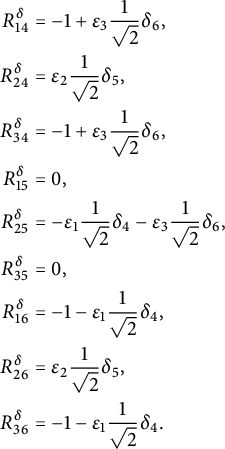 $$ \begin{align*} R_{14}^{\delta}&=-1+\varepsilon_3\frac{1}{\sqrt2}\delta_6,\\ R_{24}^{\delta}&=\varepsilon_2\frac{1}{\sqrt2}\delta_5,\\ R_{34}^{\delta}&=-1+\varepsilon_3\frac{1}{\sqrt2}\delta_6,\\ R_{15}^{\delta}&=0,\\ R_{25}^{\delta}&=-\varepsilon_1\frac{1}{\sqrt2}\delta_4-\varepsilon_3\frac{1}{\sqrt2}\delta_6,\\ R_{35}^{\delta}&=0,\\ R_{16}^{\delta}&=-1-\varepsilon_1\frac{1}{\sqrt2}\delta_4,\\ R_{26}^{\delta}&=\varepsilon_2\frac{1}{\sqrt2}\delta_5,\\ R_{36}^{\delta}&=-1-\varepsilon_{1}\frac{1}{\sqrt2}\delta_4. \end{align*} $$
This finally yields
 $ \delta _5=0 $
and
$ \delta _5=0 $
and
 $ \varepsilon _1\delta _4=-\varepsilon _3\delta _6=-\sqrt 2 $
.
$ \varepsilon _1\delta _4=-\varepsilon _3\delta _6=-\sqrt 2 $
.
Theorem 3.12 Let
 $(H,\mathcal {G}_g,\delta )$
be a generalized Einstein structure on an oriented three-dimensional unimodular Lie group G. If the endomorphism
$(H,\mathcal {G}_g,\delta )$
be a generalized Einstein structure on an oriented three-dimensional unimodular Lie group G. If the endomorphism
 $L\in \mathrm {End}\, \mathfrak g$
defined in (
24
) is diagonalizable, then there exists an oriented g-orthonormal basis
$L\in \mathrm {End}\, \mathfrak g$
defined in (
24
) is diagonalizable, then there exists an oriented g-orthonormal basis
 $(v_a)$
of
$(v_a)$
of
 $\mathfrak g = \mathrm {Lie}\, G$
and
$\mathfrak g = \mathrm {Lie}\, G$
and
 $\alpha _1,\alpha _2,\alpha _3, h \in \mathbb {R}$
such that
$\alpha _1,\alpha _2,\alpha _3, h \in \mathbb {R}$
such that
 $$ \begin{align*} [v_a,v_b] = \alpha_c \varepsilon_cv_c,\quad \forall\quad\mbox{cyclic}\quad(a,b,c)\in \mathfrak{S}_3,\quad H=h\mathrm{vol}_g, \end{align*} $$
where
 $\varepsilon _a=g(v_a,v_a)$
satisfies
$\varepsilon _a=g(v_a,v_a)$
satisfies
 $\varepsilon _1= \varepsilon _2$
. The constants
$\varepsilon _1= \varepsilon _2$
. The constants
 $(\alpha _1,\alpha _2,\alpha _3,h)$
can take the following values.
$(\alpha _1,\alpha _2,\alpha _3,h)$
can take the following values.
-
(1)
$\alpha _1=\alpha _2=\alpha _3=h=0$
, in which case
$\mathfrak g$
is abelian. The divergence can take an arbitrary value in
$ E^* $
. -
(2)
$\alpha _1=\alpha _2=\alpha _3=\pm h\neq 0$
, and
$\mathfrak g$
is isomorphic to
$\mathfrak {so}(2,1)$
or
$\mathfrak {so}(3)$
. The case
$\mathfrak {so}(3)$
occurs precisely when g is definite. Furthermore
$ \delta |_{E_{\pm }}=0 $
. -
(3) There exists a cyclic permutation
$\sigma \in \mathfrak {S}_3$
such that
$$\begin{align*}\alpha_{\sigma (1)}=\alpha_{\sigma (2)}\neq0\quad\mbox{and}\quad h=\alpha_{\sigma (3)}=0.\end{align*}$$
In this case,
$[\mathfrak g, \mathfrak g]$
is abelian of dimension
$2$
, that is,
$\mathfrak g$
is metabelian. More precisely,
$\mathfrak g$
is isomorphic to
$\mathfrak {e}(2)$
(g definite on
$ [\mathfrak {g},\mathfrak {g}] $
) or
$\mathfrak {e}(1,1)$
(g indefinite on
$ [\mathfrak {g},\mathfrak {g}] $
). The components of the divergence
$ \delta $
satisfy
$ \delta _{\sigma (1)}=\delta _{\sigma (2)}=\delta _{\sigma (1)+3}=\delta _{\sigma (2)+3}=0. $


If
 $ L $
is not diagonalizable, then
$ L $
is not diagonalizable, then
 $ h=0 $
.
$ h=0 $
.
-
(1) If
$ L $
takes the normal form
$ L_3(0,0) $
or
$ L_4(0,0) $
, then the Lie algebra
$ \mathfrak {g} $
is isomorphic to the Heisenberg algebra
$ \mathfrak {heis} $
. In this case,
$ \delta _1=\delta _4=0 $
,
$ \delta _2=\delta _3 $
and
$ \delta _5=\delta _6 $
. -
(2) If
$ L $
takes the normal form
$ L_3(\alpha ,0) $
or
$ L_4(\alpha ,0) $
,
$ \alpha \ne 0 $
, then
$ \mathfrak {g} $
is isomorphic to
$ \mathfrak {e}(1,1) $
. In these cases,
$ -\varepsilon _1\frac 12\delta _1=-\varepsilon _1\frac 12\delta _4=\alpha $
as well as
$ \delta _2=\delta _3=\delta _5=\delta _6=0 $
. -
(3) If
$ L $
takes the normal form
$ L_5(0) $
, then
$ \mathfrak {g} $
is isomorphic to
$ \mathfrak {e}(1,1) $
. In this case,
$ \varepsilon _1\delta _1=-\varepsilon _3\delta _3=\varepsilon _1\delta _4=-\varepsilon _3\delta _6=-\sqrt 2 $
and
$ \delta _2=\delta _5=0 $
.


Proof Assume first
 $ L $
is diagonalizable. To compute the components of the Ricci curvature, we use the formulas for the Dorfman coefficients and the notation for variables
$ L $
is diagonalizable. To compute the components of the Ricci curvature, we use the formulas for the Dorfman coefficients and the notation for variables
 $ X_a $
and
$ X_a $
and
 $ Y_a $
from the proof of Theorem 3.4.
$ Y_a $
from the proof of Theorem 3.4.
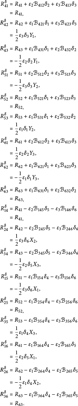 $$ \begin{align*} R_{41}^{\delta}&=R_{41}+\varepsilon_2\mathcal{B}_{412}\delta_2+\varepsilon_3\mathcal{B}_{413}\delta_3\\ &=R_{41,}\\ R_{42}^{\delta}&=R_{42}+\varepsilon_1\mathcal{B}_{421}\delta_1+\varepsilon_3\mathcal{B}_{423}\delta_3\\ &=\frac12\varepsilon_3\delta_3 Y_1,\\ R_{43}^{\delta}&=R_{43}+\varepsilon_1\mathcal{B}_{431}\delta_1+\varepsilon_2\mathcal{B}_{432}\delta_2\\ &=-\frac12\varepsilon_2\delta_2 Y_1,\\ R_{51}^{\delta}&=R_{51}+\varepsilon_2\mathcal{B}_{512}\delta_2+\varepsilon_3\mathcal{B}_{513}\delta_3\\ &=-\frac12\varepsilon_3\delta_3 Y_2,\\ R_{52}^{\delta}&=R_{52}+\varepsilon_1\mathcal{B}_{521}\delta_1+\varepsilon_3\mathcal{B}_{523}\delta_3\\ &=R_{52,}\\ R_{53}^{\delta}&=R_{53}+\varepsilon_1\mathcal{B}_{531}\delta_1+\varepsilon_2\mathcal{B}_{532}\delta_2\\ &=\frac12\varepsilon_1\delta_1 Y_2,\\ R_{61}^{\delta}&=R_{61}+\varepsilon_2\mathcal{B}_{612}\delta_2+\varepsilon_3\mathcal{B}_{613}\delta_3\\ &=\frac12\varepsilon_2\delta_2 Y_3,\\ R_{62}^{\delta}&=R_{62}+\varepsilon_1\mathcal{B}_{621}\delta_1+\varepsilon_3\mathcal{B}_{623}\delta_3\\ &=-\frac12\varepsilon_1\delta_1 Y_3,\\ R_{63}^{\delta}&=R_{63}+\varepsilon_1\mathcal{B}_{631}\delta_1+\varepsilon_2\mathcal{B}_{632}\delta_2\\ &=R_{63,}\\ R_{14}^{\delta}&=R_{41}-\varepsilon_2\mathcal{B}_{145}\delta_5-\varepsilon_3\mathcal{B}_{146}\delta_6\\ &=R_{41,}\\ R_{24}^{\delta}&=R_{42}-\varepsilon_2\mathcal{B}_{245}\delta_5-\varepsilon_3\mathcal{B}_{246}\delta_6\\ &=\frac12\varepsilon_3\delta_6 X_2,\\ R_{34}^{\delta}&=R_{43}-\varepsilon_2\mathcal{B}_{345}\delta_5-\varepsilon_3\mathcal{B}_{346}\delta_6\\ &=-\frac12\varepsilon_2\delta_5 X_3,\\ R_{15}^{\delta}&=R_{51}-\varepsilon_1\mathcal{B}_{154}\delta_4-\varepsilon_3\mathcal{B}_{156}\delta_6\\ &=-\frac12\varepsilon_3\delta_6 X_1,\\ R_{25}^{\delta}&=R_{52}-\varepsilon_1\mathcal{B}_{254}\delta_4-\varepsilon_3\mathcal{B}_{256}\delta_6\\ &=R_{52,}\\ R_{35}^{\delta}&=R_{53}-\varepsilon_1\mathcal{B}_{354}\delta_4-\varepsilon_3\mathcal{B}_{356}\delta_6\\ &=\frac12\varepsilon_1\delta_4 X_3,\\ R_{16}^{\delta}&=R_{61}-\varepsilon_1\mathcal{B}_{164}\delta_4-\varepsilon_2\mathcal{B}_{165}\delta_5\\ &=\frac12\varepsilon_2\delta_5 X_1,\\ R_{26}^{\delta}&=R_{62}-\varepsilon_1\mathcal{B}_{264}\delta_4-\varepsilon_2\mathcal{B}_{265}\delta_5\\ &=-\frac12\varepsilon_1\delta_4 X_2,\\ R_{36}^{\delta}&=R_{63}-\varepsilon_1\mathcal{B}_{364}\delta_4-\varepsilon_2\mathcal{B}_{365}\delta_5\\ &=R_{63}. \end{align*} $$
Note that if
 $(H,\mathcal G_g,\delta )$
is a generalized Einstein structure, also
$(H,\mathcal G_g,\delta )$
is a generalized Einstein structure, also
 $(H,\mathcal G_g, 0)$
is. Therefore, as in the proof of Theorem 3.4, we can distinguish cases depending on how many components of the vector
$(H,\mathcal G_g, 0)$
is. Therefore, as in the proof of Theorem 3.4, we can distinguish cases depending on how many components of the vector
 $(X_1,X_2,X_3)$
are equal to zero.
$(X_1,X_2,X_3)$
are equal to zero.
Solutions of type
 $0$
:
$0$
:
 $X_1X_2X_3\neq 0$
implies
$X_1X_2X_3\neq 0$
implies
 $ \delta _4=\delta _5=\delta _6=0 $
. Furthermore, recall that
$ \delta _4=\delta _5=\delta _6=0 $
. Furthermore, recall that
 $Y_1=Y_2=Y_3=0$
and
$Y_1=Y_2=Y_3=0$
and
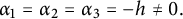 $$\begin{align*}\alpha_1=\alpha_2=\alpha_3=-h\neq0.\end{align*}$$
In this case, the Lie algebra
 $\mathfrak g$
is isomorphic to
$\mathfrak g$
is isomorphic to
 $\mathfrak {so}(2,1)$
(
$\mathfrak {so}(2,1)$
(
 $ g $
indefinite) or
$ g $
indefinite) or
 $\mathfrak {so}(3)$
(
$\mathfrak {so}(3)$
(
 $ g $
definite).
$ g $
definite).
We have seen that solutions of type
 $1$
do not exist.
$1$
do not exist.
Solutions of type
 $2$
: assume, for example, that
$2$
: assume, for example, that
 $X_1\neq 0$
,
$X_1\neq 0$
,
 $X_2=X_3=0$
. This implies
$X_2=X_3=0$
. This implies
 $ \delta _5=\delta _6=0 $
. Moreover, we have seen that
$ \delta _5=\delta _6=0 $
. Moreover, we have seen that
 $Y_2=Y_3=0$
,
$Y_2=Y_3=0$
,
 $h=\alpha _1=0$
and
$h=\alpha _1=0$
and
 $\alpha _2=\alpha _3\neq 0$
. This shows
$\alpha _2=\alpha _3\neq 0$
. This shows
 $ Y_1\neq 0 $
and thus
$ Y_1\neq 0 $
and thus
 $ \delta _2=\delta _3=0 $
. So the solutions of type
$ \delta _2=\delta _3=0 $
. So the solutions of type
 $2$
are of the following form. There exists a cyclic permutation
$2$
are of the following form. There exists a cyclic permutation
 $\sigma \in \mathfrak {S}_3$
such that
$\sigma \in \mathfrak {S}_3$
such that
 $$\begin{align*}\alpha_{\sigma (1)}=\alpha_{\sigma (2)} \neq0\quad\mbox{and}\quad h=\alpha_{\sigma (3)}=\delta_{\sigma(1)}=\delta_{\sigma(2)}=\delta_{\sigma(1)+3}=\delta_{\sigma(2)+3}=0.\end{align*}$$
As in the divergence-free case, we conclude that
 $\mathfrak g$
is metabelian. The commutator ideal
$\mathfrak g$
is metabelian. The commutator ideal
 $[\mathfrak g,\mathfrak g]= \mathrm {span}\{ v_{\sigma (1)},v_{\sigma (2)}\}$
is two-dimensional and
$[\mathfrak g,\mathfrak g]= \mathrm {span}\{ v_{\sigma (1)},v_{\sigma (2)}\}$
is two-dimensional and
 $\mathrm {ad}_{v_{\sigma (3)}}$
acts on it by a nonzero g-skew-symmetric endomorphism. This implies that
$\mathrm {ad}_{v_{\sigma (3)}}$
acts on it by a nonzero g-skew-symmetric endomorphism. This implies that
 $\mathfrak g$
is isomorphic to
$\mathfrak g$
is isomorphic to
 $\mathfrak {e}(2)$
or
$\mathfrak {e}(2)$
or
 $\mathfrak {e}(1,1)$
.
$\mathfrak {e}(1,1)$
.
Solutions of type
 $3$
: assume
$3$
: assume
 $X_1=X_2=X_3=0$
. This implies
$X_1=X_2=X_3=0$
. This implies
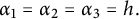 $$\begin{align*}\alpha_1=\alpha_2=\alpha_3=h.\end{align*}$$
If
 $ h=0 $
, then
$ h=0 $
, then
 $ Y_1=Y_2=Y_3=0 $
and
$ Y_1=Y_2=Y_3=0 $
and
 $ \delta \in E^* $
arbitrary, and if
$ \delta \in E^* $
arbitrary, and if
 $ h\neq 0 $
, then
$ h\neq 0 $
, then
 $ Y_1=Y_2=Y_3=2h\neq 0 $
and therefore
$ Y_1=Y_2=Y_3=2h\neq 0 $
and therefore
 $ \delta _1=\delta _2=\delta _3=0 $
.
$ \delta _1=\delta _2=\delta _3=0 $
.
By Proposition 3.11, if
 $ L $
is not diagonalizable, it is of the forms
$ L $
is not diagonalizable, it is of the forms
 $ L_3(\alpha ,0) $
,
$ L_3(\alpha ,0) $
,
 $ L_4(\alpha ,0), $
or
$ L_4(\alpha ,0), $
or
 $ L_5(0) $
and the divergence has the claimed properties. From Theorem 3.4, we know that
$ L_5(0) $
and the divergence has the claimed properties. From Theorem 3.4, we know that
 $ G $
is the Heisenberg group if
$ G $
is the Heisenberg group if
 $ L $
takes the normal for
$ L $
takes the normal for
 $ L_3(0,0) $
or
$ L_3(0,0) $
or
 $ L_4(0,0) $
. If
$ L_4(0,0) $
. If
 $ \alpha \ne 0 $
,
$ \alpha \ne 0 $
,
 $\mathrm {ad}_{v_1}$
acts on
$\mathrm {ad}_{v_1}$
acts on
 $[\mathfrak g,\mathfrak g]= \mathrm {span}\{ v_2,v_3\}$
by a symmetric endomorphism with eigenvalues
$[\mathfrak g,\mathfrak g]= \mathrm {span}\{ v_2,v_3\}$
by a symmetric endomorphism with eigenvalues
 $ \alpha $
and
$ \alpha $
and
 $ -\alpha $
. Therefore
$ -\alpha $
. Therefore
 $ \mathfrak {g}\cong \mathfrak {e}(1,1) $
.
$ \mathfrak {g}\cong \mathfrak {e}(1,1) $
.
If
 $ L $
takes the normal form
$ L $
takes the normal form
 $ L_5(0) $
, one can show that the only unimodular Lie algebra whose Killing form has the same signature as the one of
$ L_5(0) $
, one can show that the only unimodular Lie algebra whose Killing form has the same signature as the one of
 $ \mathfrak {g} $
, is the Lie algebra
$ \mathfrak {g} $
, is the Lie algebra
 $ \mathfrak {e}(1,1) $
. Alternatively, one can check that
$ \mathfrak {e}(1,1) $
. Alternatively, one can check that
 $\mathrm {ad}_{v_1+v_3}$
acts on
$\mathrm {ad}_{v_1+v_3}$
acts on
 $ \mathrm {span}\{ v_2,v_1-v_3\} $
a symmetric endomorphism with eigenvalues
$ \mathrm {span}\{ v_2,v_1-v_3\} $
a symmetric endomorphism with eigenvalues
 $ \sqrt 2 $
and
$ \sqrt 2 $
and
 $ -\sqrt 2 $
. Therefore again
$ -\sqrt 2 $
. Therefore again
 $ \mathfrak {g}\cong \mathfrak {e}(1,1) $
.
$ \mathfrak {g}\cong \mathfrak {e}(1,1) $
.
Remark 3.13 Except for the cases that the endomorphism
 $ L $
takes the normal form
$ L $
takes the normal form
 $ L_3(\alpha ,0)$
,
$ L_3(\alpha ,0)$
,
 $L_4(\alpha ,0) $
(
$L_4(\alpha ,0) $
(
 $ \alpha \ne 0 $
), and
$ \alpha \ne 0 $
), and
 $ L_5(0) $
, the solutions are such that the Ricci tensor for zero divergence and the contribution of the divergence to the Ricci tensor vanish simultaneously.
$ L_5(0) $
, the solutions are such that the Ricci tensor for zero divergence and the contribution of the divergence to the Ricci tensor vanish simultaneously.
Corollary 3.14 Let
 $(H,\mathcal {G}_g,\delta )$
be a generalized Einstein structure on a three-dimensional Lie group G. Then the left-invariant metric defined by g is bi-invariant if and only if
$(H,\mathcal {G}_g,\delta )$
be a generalized Einstein structure on a three-dimensional Lie group G. Then the left-invariant metric defined by g is bi-invariant if and only if
 $\mathfrak {g}$
is isomorphic to
$\mathfrak {g}$
is isomorphic to
 $\mathfrak {so}(3)$
,
$\mathfrak {so}(3)$
,
 $\mathfrak {so}(2,1)$
or
$\mathfrak {so}(2,1)$
or
 $\mathbb {R}^3$
.
$\mathbb {R}^3$
.
Proof This follows from the fact that the only three-dimensional Lie algebras admitting an ad-invariant scalar product are the above three Lie algebras together with our classification of generalized Einstein structures on these Lie algebras.
3.3.2 Non-unimodular Lie groups
Proposition 3.15 Let
 $(H,\mathcal G_g,\delta )$
be a generalized Einstein structure on a three-dimensional nonunimodular Lie group G. Let
$(H,\mathcal G_g,\delta )$
be a generalized Einstein structure on a three-dimensional nonunimodular Lie group G. Let
 $ \mathfrak {u} $
be the unimodular kernel of the Lie algebra
$ \mathfrak {u} $
be the unimodular kernel of the Lie algebra
 $ \mathfrak {g} $
and assume that
$ \mathfrak {g} $
and assume that
 $ g|_{\mathfrak {u}\times \mathfrak {u}} $
is nondegenerate. Then there exists an orthonormal basis
$ g|_{\mathfrak {u}\times \mathfrak {u}} $
is nondegenerate. Then there exists an orthonormal basis
 $(v_a)$
of
$(v_a)$
of
 $(\mathfrak {g},g)$
such that
$(\mathfrak {g},g)$
such that
 $ v_1,v_3\in \mathfrak {u} $
and
$ v_1,v_3\in \mathfrak {u} $
and
 $g(v_1,v_1)=g(v_2,v_2)=-g(v_3,v_3)$
. Furthermore
$g(v_1,v_1)=g(v_2,v_2)=-g(v_3,v_3)$
. Furthermore
 $\delta _2=\delta _5$
. If
$\delta _2=\delta _5$
. If
 $ \delta _2=\delta _5=0 $
, then
$ \delta _2=\delta _5=0 $
, then
 $\delta =0$
,
$\delta =0$
,
 $ h=0 $
and one can choose
$ h=0 $
and one can choose
 $ v_1 $
and
$ v_1 $
and
 $ v_3 $
such that there is a positive constant
$ v_3 $
such that there is a positive constant
 $ \theta>0 $
such that
$ \theta>0 $
such that
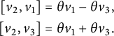 $$ \begin{align*} \left[v_2,v_1\right]&=\theta v_1-\theta v_3,\\ \left[v_2,v_3\right]&=\theta v_1+\theta v_3. \end{align*} $$
If
 $ \delta _2=\delta _5\neq 0 $
,
$ \delta _2=\delta _5\neq 0 $
,
![]() is diagonalizable. We have
is diagonalizable. We have
 $ h^2=\left (\operatorname {\mathrm{tr}} M\right )^2\ne 0 $
and
$ h^2=\left (\operatorname {\mathrm{tr}} M\right )^2\ne 0 $
and
 $ \delta _2=\delta _5=-\operatorname {\mathrm{tr}} M \ne 0 $
. In the special case that
$ \delta _2=\delta _5=-\operatorname {\mathrm{tr}} M \ne 0 $
. In the special case that
 $ M $
has a double eigenvalue, it is diagonalizable by an orthonormal basis. That is, one can choose
$ M $
has a double eigenvalue, it is diagonalizable by an orthonormal basis. That is, one can choose
 $ v_1 $
and
$ v_1 $
and
 $ v_3 $
such that there exists a positive constant
$ v_3 $
such that there exists a positive constant
 $ \theta>0 $
such that
$ \theta>0 $
such that
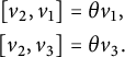 $$ \begin{align*} \left[v_2,v_1\right]&=\theta v_1,\\ \left[v_2,v_3\right]&=\theta v_3. \end{align*} $$
In this case,
 $ h^2=\left (2\theta \right )^2\ne 0 $
and
$ h^2=\left (2\theta \right )^2\ne 0 $
and
 $ \delta _2=\delta _5=-2\theta \ne 0 $
. Furthermore
$ \delta _2=\delta _5=-2\theta \ne 0 $
. Furthermore
 $ \delta _1=\delta _3=\delta _4=\delta _6=0 $
. In the case
$ \delta _1=\delta _3=\delta _4=\delta _6=0 $
. In the case
 $ \delta _2=\delta _5\neq 0 $
and two distinct real eigenvalues of
$ \delta _2=\delta _5\neq 0 $
and two distinct real eigenvalues of
 $M,$
there are the following families of solutions of the generalized Einstein equation:
$M,$
there are the following families of solutions of the generalized Einstein equation:
-
(1)
$h=\pm 2\lambda $
,
$\delta _2=\delta _5= -2\varepsilon _2\lambda $
and
$\delta _1=\delta _3=\delta _4=\delta _6=0$
,
$$\begin{align*}M=\left( \begin{array}{cc} \varepsilon_1\lambda &-\varepsilon_1\mu\\ \varepsilon_3\mu&-\varepsilon_{3}\lambda \end{array} \right), \end{align*}$$
where
$\lambda ,\mu \in \mathbb {R}\setminus \{0\}$
and
$|\mu |\neq |\lambda |$
. -
2A.
$h=\mu -\nu $
,
$\delta _2=\delta _5=\varepsilon _2(-\mu +\nu )$
,
$\delta _4=\delta _6=0$
,
$\delta _1$
and
$\delta _3$
are related by
$\mu \delta _1-\nu \delta _3=0$
and
$$\begin{align*}M=\left( \begin{array}{cc} \varepsilon_1\mu&\varepsilon_1\nu\\ \varepsilon_3\mu&\varepsilon_{3}\nu \end{array} \right), \end{align*}$$
where
$\mu , \nu \in \mathbb {R}$
are such that
$\mu -\nu \neq 0$
. -
2B.
$h=\mu -\nu $
,
$\delta _2=\delta _5=\varepsilon _2(\mu -\nu )$
,
$\delta _4=\delta _6=0$
,
$\delta _1$
and
$\delta _3$
are related by
$\mu \delta _1+\nu \delta _3=0$
and
$$\begin{align*}M=\left( \begin{array}{cc}-\varepsilon_1\mu &\varepsilon_1\nu\\ \varepsilon_3\mu&-\varepsilon_{3}\nu \end{array} \right), \end{align*}$$
where
$\mu , \nu \in \mathbb {R}$
are such that
$\mu -\nu \neq 0$
. -
2C.
$h=2\mu $
,
$\delta _2=\delta _5=2\varepsilon _2 \mu $
,
$\delta _1=\delta _3$
,
$\delta _4=\delta _6=0$
and
$$\begin{align*}M=\left( \begin{array}{cc}-\varepsilon_1\mu &-\varepsilon_1\mu\\ \varepsilon_3\mu &\varepsilon_{3}\mu \end{array} \right), \end{align*}$$
where
$\mu \in \mathbb {R}\setminus \{0\}$
. -
2D.
$h=2\mu $
,
$\delta _2=\delta _5= -2\varepsilon _2\mu $
,
$\delta _1=-\delta _3$
,
$\delta _4=\delta _6=0$
and
$$\begin{align*}M=\left( \begin{array}{cc}\varepsilon_1\mu&-\varepsilon_1\mu\\ \varepsilon_3\mu&-\varepsilon_{3}\mu \end{array} \right), \end{align*}$$
where
$\mu \in \mathbb {R}\setminus \{ 0\}$
. -
3A.
$h=\nu -\mu $
,
$\delta _2=\delta _5= \varepsilon _2(\nu -\mu )$
,
$\delta _1=\delta _3=0$
,
$\delta _4$
and
$\delta _6$
are related by
$\mu \delta _4-\nu \delta _6=0$
and
$$\begin{align*}M=\left( \begin{array}{cc}\varepsilon_1\mu& \varepsilon_1\nu \\ \varepsilon_3\mu&\varepsilon_{3}\nu \end{array} \right), \end{align*}$$
where
$\mu , \nu \in \mathbb {R}$
are such that
$\mu -\nu \neq 0$
. -
3B.
$h=\nu -\mu $
,
$\delta _2=\delta _5= \varepsilon _2(\mu -\nu )$
,
$\delta _1=\delta _3=0$
,
$\delta _4$
and
$\delta _6$
are related by
$\mu \delta _4+\nu \delta _6=0$
and
$$\begin{align*}M=\left( \begin{array}{cc} -\varepsilon_1\mu&\varepsilon_1\nu\\ \varepsilon_3\mu&-\varepsilon_{3}\nu \end{array} \right), \end{align*}$$
where
$\mu , \nu \in \mathbb {R}$
are such that
$\mu -\nu \neq 0$
. -
3C.
$h=-2\mu $
,
$\delta _2=\delta _5= 2\varepsilon _2\mu $
,
$\delta _1=\delta _3=0$
,
$\delta _4=\delta _6$
and
$$\begin{align*}M=\left( \begin{array}{cc}-\varepsilon_1\mu &-\varepsilon_1\mu\\ \varepsilon_3\mu &\varepsilon_{3}\mu \end{array} \right), \end{align*}$$
where
$\mu \in \mathbb {R}\setminus \{ 0\}$
. -
3D.
$h=-2\mu $
,
$\delta _2=\delta _5= -2\varepsilon _2\mu $
,
$\delta _1=\delta _3=0$
,
$\delta _4=-\delta _6$
and
$$\begin{align*}M=\left( \begin{array}{cc} \varepsilon_1\mu &-\varepsilon_1\mu \\ \varepsilon_3\mu &-\varepsilon_{3}\mu \end{array} \right), \end{align*}$$
where
$\mu \in \mathbb {R}\setminus \{ 0\}$
.


Proof As in the proof of Proposition 3.5, there exists a
 $ g $
-orthonormal basis
$ g $
-orthonormal basis
 $ (v_a)_a $
of
$ (v_a)_a $
of
 $ \mathfrak g $
such that
$ \mathfrak g $
such that
 $ v_1,v_3\in \mathfrak {u} $
and
$ v_1,v_3\in \mathfrak {u} $
and
 $ \lambda ,\mu ,\nu ,\rho \in \mathbb {R} $
such that
$ \lambda ,\mu ,\nu ,\rho \in \mathbb {R} $
such that
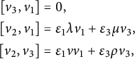 $$ \begin{align*} [v_3,v_1]&= 0,\\ \left[v_2,v_1\right]&=\varepsilon_1\lambda v_1+\varepsilon_3\mu v_3,\\ \left[v_2,v_3\right]&=\varepsilon_1\nu v_1+\varepsilon_{3}\rho v_3, \end{align*} $$
with
 $ 0\neq \operatorname {\mathrm{tr}} \mathrm {ad}_{v_2}=\varepsilon _1\lambda +\varepsilon _{3}\rho $
. Using the Dorfman coefficients, that were computed in the proof of Proposition 3.5, we obtain the components of the Ricci tensor.
$ 0\neq \operatorname {\mathrm{tr}} \mathrm {ad}_{v_2}=\varepsilon _1\lambda +\varepsilon _{3}\rho $
. Using the Dorfman coefficients, that were computed in the proof of Proposition 3.5, we obtain the components of the Ricci tensor.
In the case
 $ \varepsilon _1=\varepsilon _3 $
, we have
$ \varepsilon _1=\varepsilon _3 $
, we have
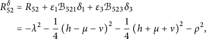 $$ \begin{align*} R^{\delta}_{52}&=R_{52}+\varepsilon_1\mathcal{B}_{521}\delta_1+\varepsilon_3\mathcal{B}_{523}\delta_3\\ &=-\lambda^2-\frac14\left(h-\mu-\nu\right)^2-\frac14\left(h+\mu+\nu\right)^2-\rho^2, \end{align*} $$
which is always nonzero due to
 $ 0\neq \varepsilon _1\lambda +\varepsilon _{3}\rho $
. Hence, we can assume that the basis is chosen such that
$ 0\neq \varepsilon _1\lambda +\varepsilon _{3}\rho $
. Hence, we can assume that the basis is chosen such that
 $ \varepsilon _{1}=\varepsilon _{2}=-\varepsilon _{3} $
.
$ \varepsilon _{1}=\varepsilon _{2}=-\varepsilon _{3} $
.
In this case, the components of the Ricci tensor are
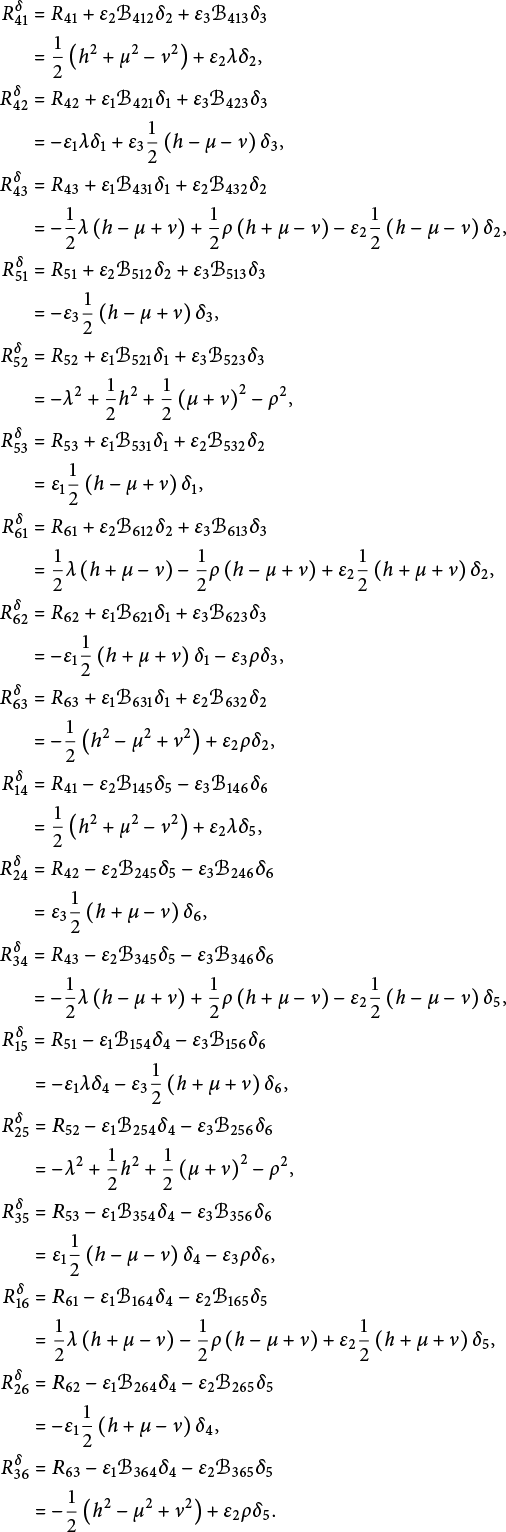 $$ \begin{align*} R_{41}^{\delta}&=R_{41}+\varepsilon_2\mathcal{B}_{412}\delta_2+\varepsilon_3\mathcal{B}_{413}\delta_3\\ &=\frac12\left(h^2+\mu^2-\nu^2\right)+\varepsilon_2\lambda\delta_2,\\ R_{42}^{\delta}&=R_{42}+\varepsilon_1\mathcal{B}_{421}\delta_1+\varepsilon_3\mathcal{B}_{423}\delta_3\\ &=-\varepsilon_1\lambda\delta_1+\varepsilon_3\frac12\left(h-\mu-\nu\right)\delta_3,\\ R_{43}^{\delta}&=R_{43}+\varepsilon_1\mathcal{B}_{431}\delta_1+\varepsilon_2\mathcal{B}_{432}\delta_2\\ &=-\frac12\lambda\left(h-\mu+\nu\right)+\frac12\rho\left(h+\mu-\nu\right)-\varepsilon_2\frac12\left(h-\mu-\nu\right)\delta_2,\\ R_{51}^{\delta}&=R_{51}+\varepsilon_2\mathcal{B}_{512}\delta_2+\varepsilon_3\mathcal{B}_{513}\delta_3\\ &=-\varepsilon_3\frac12\left(h-\mu+\nu\right)\delta_3,\\ R_{52}^{\delta}&=R_{52}+\varepsilon_1\mathcal{B}_{521}\delta_1+\varepsilon_3\mathcal{B}_{523}\delta_3\\ &=-\lambda^2+\frac12h^2+\frac12\left(\mu+\nu\right)^2-\rho^2,\\ R_{53}^{\delta}&=R_{53}+\varepsilon_1\mathcal{B}_{531}\delta_1+\varepsilon_2\mathcal{B}_{532}\delta_2\\ &=\varepsilon_1\frac12\left(h-\mu+\nu\right)\delta_1,\\ R_{61}^{\delta}&=R_{61}+\varepsilon_2\mathcal{B}_{612}\delta_2+\varepsilon_3\mathcal{B}_{613}\delta_3\\ &=\frac12\lambda\left(h+\mu-\nu\right)-\frac12\rho\left(h-\mu+\nu\right)+\varepsilon_2\frac12\left(h+\mu+\nu\right)\delta_2,\\ R_{62}^{\delta}&=R_{62}+\varepsilon_1\mathcal{B}_{621}\delta_1+\varepsilon_3\mathcal{B}_{623}\delta_3\\ &=-\varepsilon_1\frac12\left(h+\mu+\nu\right)\delta_1-\varepsilon_3\rho\delta_3,\\ R_{63}^{\delta}&=R_{63}+\varepsilon_1\mathcal{B}_{631}\delta_1+\varepsilon_2\mathcal{B}_{632}\delta_2\\ &=-\frac12\left(h^2-\mu^2+\nu^2\right)+\varepsilon_2\rho\delta_2,\\ R_{14}^{\delta}&=R_{41}-\varepsilon_2\mathcal{B}_{145}\delta_5-\varepsilon_3\mathcal{B}_{146}\delta_6\\ &=\frac12\left(h^2+\mu^2-\nu^2\right)+\varepsilon_2\lambda\delta_5,\\ R_{24}^{\delta}&=R_{42}-\varepsilon_2\mathcal{B}_{245}\delta_5-\varepsilon_3\mathcal{B}_{246}\delta_6\\ &=\varepsilon_3\frac12\left(h+\mu-\nu\right)\delta_6,\\ R_{34}^{\delta}&=R_{43}-\varepsilon_2\mathcal{B}_{345}\delta_5-\varepsilon_3\mathcal{B}_{346}\delta_6\\ &=-\frac12\lambda\left(h-\mu+\nu\right)+\frac12\rho\left(h+\mu-\nu\right)-\varepsilon_2\frac12\left(h-\mu-\nu\right)\delta_5,\\ R_{15}^{\delta}&=R_{51}-\varepsilon_1\mathcal{B}_{154}\delta_4-\varepsilon_3\mathcal{B}_{156}\delta_6\\ &=-\varepsilon_1\lambda\delta_4-\varepsilon_3\frac12\left(h+\mu+\nu\right)\delta_6,\\ R_{25}^{\delta}&=R_{52}-\varepsilon_1\mathcal{B}_{254}\delta_4-\varepsilon_3\mathcal{B}_{256}\delta_6\\ &=-\lambda^2+\frac12h^2+\frac12\left(\mu+\nu\right)^2-\rho^2,\\ R_{35}^{\delta}&=R_{53}-\varepsilon_1\mathcal{B}_{354}\delta_4-\varepsilon_3\mathcal{B}_{356}\delta_6\\ &=\varepsilon_1\frac12\left(h-\mu-\nu\right)\delta_4-\varepsilon_3\rho\delta_6,\\ R_{16}^{\delta}&=R_{61}-\varepsilon_1\mathcal{B}_{164}\delta_4-\varepsilon_2\mathcal{B}_{165}\delta_5\\ &=\frac12\lambda\left(h+\mu-\nu\right)-\frac12\rho\left(h-\mu+\nu\right)+\varepsilon_2\frac12\left(h+\mu+\nu\right)\delta_5,\\ R_{26}^{\delta}&=R_{62}-\varepsilon_1\mathcal{B}_{264}\delta_4-\varepsilon_2\mathcal{B}_{265}\delta_5\\ &=-\varepsilon_1\frac12\left(h+\mu-\nu\right)\delta_4,\\ R_{36}^{\delta}&=R_{63}-\varepsilon_1\mathcal{B}_{364}\delta_4-\varepsilon_2\mathcal{B}_{365}\delta_5\\ &=-\frac12\left(h^2-\mu^2+\nu^2\right)+\varepsilon_2\rho\delta_5.\end{align*} $$
Note first that
 $ R_{41}^{\delta }=R_{14}^{\delta } $
and
$ R_{41}^{\delta }=R_{14}^{\delta } $
and
 $ R_{63}^{\delta }=R_{36}^{\delta } $
yield
$ R_{63}^{\delta }=R_{36}^{\delta } $
yield
 $ \varepsilon _2\lambda \left (\delta _2-\delta _5\right )=0 $
and
$ \varepsilon _2\lambda \left (\delta _2-\delta _5\right )=0 $
and
 $ \varepsilon _2\rho \left (\delta _2-\delta _5\right )=0 $
. Therefore
$ \varepsilon _2\rho \left (\delta _2-\delta _5\right )=0 $
. Therefore
 $ \delta _2=\delta _5 $
, because
$ \delta _2=\delta _5 $
, because
 $ 0\neq \varepsilon _1\lambda +\varepsilon _{3}\rho $
. If
$ 0\neq \varepsilon _1\lambda +\varepsilon _{3}\rho $
. If
 $ \delta _2=\delta _5=0 $
, we see that
$ \delta _2=\delta _5=0 $
, we see that
 $ R_{ii'}^{\delta }=R_{i'i}^{\delta }=R_{ii'} $
for all
$ R_{ii'}^{\delta }=R_{i'i}^{\delta }=R_{ii'} $
for all
 $ i\in \{4,5,6\} $
. So we can deduce the same way as in the proof of Proposition 3.5, that
$ i\in \{4,5,6\} $
. So we can deduce the same way as in the proof of Proposition 3.5, that
 $ h=0 $
and there is a positive constant
$ h=0 $
and there is a positive constant
 $ \theta>0 $
such that
$ \theta>0 $
such that
 $ \varepsilon _1\lambda =-\varepsilon _3\mu =\varepsilon _1\nu =\varepsilon _3\rho =\theta $
. Then we see that
$ \varepsilon _1\lambda =-\varepsilon _3\mu =\varepsilon _1\nu =\varepsilon _3\rho =\theta $
. Then we see that
 $ 0=R_{42}^{\delta }=-\theta \delta _1+\theta \delta _3 $
and
$ 0=R_{42}^{\delta }=-\theta \delta _1+\theta \delta _3 $
and
 $ R_{15}^{\delta }=-\theta \delta _4+\theta \delta _6 $
imply
$ R_{15}^{\delta }=-\theta \delta _4+\theta \delta _6 $
imply
 $ \delta _1=\delta _3 $
and
$ \delta _1=\delta _3 $
and
 $ \delta _4=\delta _6 $
. Similarly,
$ \delta _4=\delta _6 $
. Similarly,
 $R_{62}^{\delta }=-\theta \delta _1 -\theta \delta _3=0$
and
$R_{62}^{\delta }=-\theta \delta _1 -\theta \delta _3=0$
and
 $R_{35}^{\delta }=-\theta \delta _4-\theta \delta _6=0$
imply
$R_{35}^{\delta }=-\theta \delta _4-\theta \delta _6=0$
imply
 $ \delta _1=-\delta _3 $
and
$ \delta _1=-\delta _3 $
and
 $ \delta _4=-\delta _6 $
. This proves that
$ \delta _4=-\delta _6 $
. This proves that
 $\delta =0$
if
$\delta =0$
if
 $\delta _2=\delta _5=0$
. Note that the endomorphism
$\delta _2=\delta _5=0$
. Note that the endomorphism
 $ M\in \operatorname {\mathrm {End}}(\mathfrak {u}) $
, defined as the restriction of
$ M\in \operatorname {\mathrm {End}}(\mathfrak {u}) $
, defined as the restriction of
 $ \mathrm {ad}_{v_2} $
to
$ \mathrm {ad}_{v_2} $
to
 $ \mathfrak {u} $
, has the two complex eigenvalues
$ \mathfrak {u} $
, has the two complex eigenvalues
 $ \theta \pm i\theta $
. Assume now
$ \theta \pm i\theta $
. Assume now
 $ \delta _2=\delta _5\neq 0 $
. Then
$ \delta _2=\delta _5\neq 0 $
. Then
 $$ \begin{align} 0=R_{41}^{\delta}-R_{63}^{\delta}=h^2+\varepsilon_2\delta_2\left(\lambda-\rho\right). \end{align} $$
Using
 $ \lambda -\rho =\varepsilon _1\left (\varepsilon _1\lambda +\varepsilon _3\rho \right )\neq 0 $
, we see
$ \lambda -\rho =\varepsilon _1\left (\varepsilon _1\lambda +\varepsilon _3\rho \right )\neq 0 $
, we see
 $ h\neq 0 $
. From
$ h\neq 0 $
. From
 $ 0=R_{61}^{\delta }-R_{43}^{\delta }=h\left (\lambda -\rho +\varepsilon _2\delta _2\right ) $
, we see
$ 0=R_{61}^{\delta }-R_{43}^{\delta }=h\left (\lambda -\rho +\varepsilon _2\delta _2\right ) $
, we see
 $ \varepsilon _2\delta _2=-\lambda +\rho =-\varepsilon _2\operatorname {\mathrm{tr}} M $
. Then equation (29) is equivalent to
$ \varepsilon _2\delta _2=-\lambda +\rho =-\varepsilon _2\operatorname {\mathrm{tr}} M $
. Then equation (29) is equivalent to
 $ h^2=\left (\lambda -\rho \right )^2=\left (\operatorname {\mathrm{tr}} M\right )^2 $
. Since
$ h^2=\left (\lambda -\rho \right )^2=\left (\operatorname {\mathrm{tr}} M\right )^2 $
. Since
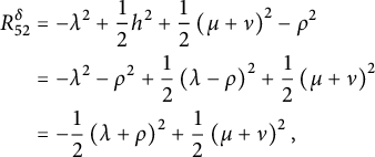 $$ \begin{align*} R_{52}^{\delta}&=-\lambda^2+\frac12h^2+\frac12\left(\mu+\nu\right)^2-\rho^2\\ &=-\lambda^2-\rho^2+\frac12\left(\lambda-\rho\right)^2+\frac12\left(\mu+\nu\right)^2\\ &=-\frac12\left(\lambda+\rho\right)^2+\frac12\left(\mu+\nu\right)^2, \end{align*} $$
the equation
 $ R_{52}^{\delta }=0 $
is equivalent to
$ R_{52}^{\delta }=0 $
is equivalent to
 $$ \begin{align} \left(\lambda+\rho\right)^2=\left(\mu+\nu\right)^2. \end{align} $$
Note now that the discriminant
 $ \Delta $
of the characteristic polynomial
$ \Delta $
of the characteristic polynomial
 $ X^2-\varepsilon _1\left (\lambda -\rho \right )X-\lambda \rho +\mu \nu $
of
$ X^2-\varepsilon _1\left (\lambda -\rho \right )X-\lambda \rho +\mu \nu $
of
 $ M $
is
$ M $
is
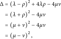 $$ \begin{align*} \Delta&=\left(\lambda-\rho\right)^2+4\lambda\rho-4\mu\nu\\ &=\left(\lambda+\rho\right)^2-4\mu\nu\\ &=\left(\mu+\nu\right)^2-4\mu\nu\\ &=\left(\mu-\nu\right)^2, \end{align*} $$
which is never negative. Therefore,
 $ M $
has real eigenvalues. Hence,
$ M $
has real eigenvalues. Hence,
 $ M $
is either diagonalizable with two distinct eigenvalues, or it has a double eigenvalue. The latter happens precisely if the discriminant is zero, that is, if
$ M $
is either diagonalizable with two distinct eigenvalues, or it has a double eigenvalue. The latter happens precisely if the discriminant is zero, that is, if
 $ \mu =\nu $
. But then,
$ \mu =\nu $
. But then,
 $ M $
is a symmetric endomorphism and hence takes one of the normal forms
$ M $
is a symmetric endomorphism and hence takes one of the normal forms
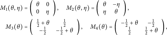 $$ \begin{align*} M_1(\theta,\eta ) &= \left( \begin{array}{cc} \theta& 0\\ 0&\eta \end{array}\right),\quad M_2(\theta,\eta )=\left( \begin{array}{cc} \theta& -\eta\\ \eta&\theta \end{array}\right),\\ M_3(\theta)&=\left( \begin{array}{cc}\frac12+\theta &\frac12\\ -\frac12&-\frac12 +\theta \end{array}\right),\quad M_4(\theta)= \left( \begin{array}{cc} -\frac12+\theta &-\frac12\\ \frac12&\frac12 +\theta\\ \end{array}\right), \end{align*} $$
with respect to an orthonormal basis
 $ v_1,v_3 $
of
$ v_1,v_3 $
of
 $ \mathfrak {u} $
, as in the proof of Proposition 3.5. If it takes the normal form
$ \mathfrak {u} $
, as in the proof of Proposition 3.5. If it takes the normal form
 $ M_1(\theta ,\eta ) $
, then
$ M_1(\theta ,\eta ) $
, then
 $ \theta =\eta $
, since
$ \theta =\eta $
, since
 $ M $
has a double eigenvalue. Hence, that
$ M $
has a double eigenvalue. Hence, that
 $ M $
is of the form
$ M $
is of the form
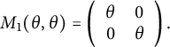 $$ \begin{align*} M_1(\theta,\theta)=\left( \begin{array}{cc} \theta& 0\\ 0 &\theta \end{array}\right). \end{align*} $$
We may assume
 $ \theta $
is positive by replacing
$ \theta $
is positive by replacing
 $ v_2 $
with
$ v_2 $
with
 $ -v_2 $
. If it takes the normal form
$ -v_2 $
. If it takes the normal form
 $ M_2(\theta ,\eta ) $
, then we have
$ M_2(\theta ,\eta ) $
, then we have
 $ R_{43}^{\delta }+R_{61}^{\delta }=-2\theta \eta $
. But
$ R_{43}^{\delta }+R_{61}^{\delta }=-2\theta \eta $
. But
 $ \theta \ne 0 $
, since
$ \theta \ne 0 $
, since
 $ \operatorname {\mathrm{tr}} M \ne 0 $
. Therefore,
$ \operatorname {\mathrm{tr}} M \ne 0 $
. Therefore,
 $ \eta =0 $
and we get the same normal form as before. The normal forms
$ \eta =0 $
and we get the same normal form as before. The normal forms
 $ M_3(\theta ) $
and
$ M_3(\theta ) $
and
 $ M_4(\theta ) $
are excluded, because in both cases
$ M_4(\theta ) $
are excluded, because in both cases
 $ R_{43}^{\delta }+R_{61}^{\delta }=2\theta $
, which cannot be zero because
$ R_{43}^{\delta }+R_{61}^{\delta }=2\theta $
, which cannot be zero because
 $ \operatorname {\mathrm{tr}} M \ne 0 $
. Note that in the case that
$ \operatorname {\mathrm{tr}} M \ne 0 $
. Note that in the case that
 $ M $
takes the normal form
$ M $
takes the normal form
 $ M_1(\theta ,\theta ) $
, we have
$ M_1(\theta ,\theta ) $
, we have
 $ \delta _1=\delta _3=\delta _4=\delta _6=0 $
, due to
$ \delta _1=\delta _3=\delta _4=\delta _6=0 $
, due to
 $ R_{53}^{\delta }=R_{51}^{\delta }=R_{26}^{\delta }=R_{24}^{\delta }=0 $
.
$ R_{53}^{\delta }=R_{51}^{\delta }=R_{26}^{\delta }=R_{24}^{\delta }=0 $
.
It remains to consider the case
 $\mu -\nu \neq 0$
. Recall that
$\mu -\nu \neq 0$
. Recall that
 $\delta _2=\delta _5 = \varepsilon _2(-\lambda +\rho )\neq 0$
and
$\delta _2=\delta _5 = \varepsilon _2(-\lambda +\rho )\neq 0$
and
 $h=\pm (\lambda -\rho )\neq 0$
. We distinguish the following cases. Note that the expressions
$h=\pm (\lambda -\rho )\neq 0$
. We distinguish the following cases. Note that the expressions
 $h-\mu +\nu $
and
$h-\mu +\nu $
and
 $h+\mu -\nu $
cannot both vanish simultaneously, since
$h+\mu -\nu $
cannot both vanish simultaneously, since
 $h\neq 0.$
Case 1:
 $h-\mu +\nu \neq 0$
and
$h-\mu +\nu \neq 0$
and
 $h+\mu -\nu \neq 0$
. In this case, we conclude from
$h+\mu -\nu \neq 0$
. In this case, we conclude from
 $R_{51}^{\delta }= R_{53}^{\delta }=R_{24}^{\delta }=R_{26}^{\delta }=0$
that
$R_{51}^{\delta }= R_{53}^{\delta }=R_{24}^{\delta }=R_{26}^{\delta }=0$
that
 $\delta _1=\delta _3=\delta _4=\delta _6=0$
. Then from the remaining equations, we obtain
$\delta _1=\delta _3=\delta _4=\delta _6=0$
. Then from the remaining equations, we obtain
 $$\begin{align*}\mu^2 -\lambda^2 =-(\rho^2-\nu^2),\; \rho\mu-\lambda\nu=0,\; (\lambda+\rho)^2 = (\mu +\nu)^2.\end{align*}$$
The first two equations are satisfied if and only if
 $(\mu ,\lambda )$
and
$(\mu ,\lambda )$
and
 $(\rho , \nu )$
are nonzero orthogonal vectors of equal length in the Minkowski plane. This implies that
$(\rho , \nu )$
are nonzero orthogonal vectors of equal length in the Minkowski plane. This implies that
 $(\mu ,\lambda )= - (\nu ,\rho )$
, since
$(\mu ,\lambda )= - (\nu ,\rho )$
, since
 $\mu -\nu \neq 0$
. This yields the first family of solutions for which M has two distinct real eigenvalues.
$\mu -\nu \neq 0$
. This yields the first family of solutions for which M has two distinct real eigenvalues.
Case 2:
 $h-\mu +\nu = 0$
and
$h-\mu +\nu = 0$
and
 $h+\mu -\nu \neq 0$
. In this case, the equations
$h+\mu -\nu \neq 0$
. In this case, the equations
 $R_{51}^{\delta }= R_{53}^{\delta }=R_{24}^{\delta }=R_{26}^{\delta }=0$
reduce to
$R_{51}^{\delta }= R_{53}^{\delta }=R_{24}^{\delta }=R_{26}^{\delta }=0$
reduce to
 $\delta _4=\delta _6=0$
. Recall that
$\delta _4=\delta _6=0$
. Recall that
 $R_{52}^{\delta }=0$
yields equation (30) and hence
$R_{52}^{\delta }=0$
yields equation (30) and hence
 $\mu +\nu = \sigma _+ (\lambda +\rho )$
for some
$\mu +\nu = \sigma _+ (\lambda +\rho )$
for some
 $\sigma _+\in \{ \pm 1\}$
. Since now
$\sigma _+\in \{ \pm 1\}$
. Since now
 $h=\mu -\nu $
, the equation
$h=\mu -\nu $
, the equation
 $h^2 = (\lambda -\rho )^2$
yields
$h^2 = (\lambda -\rho )^2$
yields
 $\mu -\nu = \sigma _-(\lambda -\rho )$
,
$\mu -\nu = \sigma _-(\lambda -\rho )$
,
 $\sigma _-\in \{\pm 1\}$
. We consider four subcases depending on the signs
$\sigma _-\in \{\pm 1\}$
. We consider four subcases depending on the signs
 $\sigma _{\pm }$
. In each case, we first solve the two equations
$\sigma _{\pm }$
. In each case, we first solve the two equations
 $\mu \pm \nu = \sigma _{\pm } (\lambda \pm \rho )$
.
$\mu \pm \nu = \sigma _{\pm } (\lambda \pm \rho )$
.
Case 2A:
 $\sigma _+=\sigma _-=1$
. In this case,
$\sigma _+=\sigma _-=1$
. In this case,
 $\mu =\lambda $
and
$\mu =\lambda $
and
 $\nu = \rho $
. It turns out that the remaining components of the generalized Ricci curvature vanish if
$\nu = \rho $
. It turns out that the remaining components of the generalized Ricci curvature vanish if
 $R_{42}^{\delta }$
does. Its vanishing is equivalent to
$R_{42}^{\delta }$
does. Its vanishing is equivalent to
 $\mu \delta _1-\nu \delta _3=0$
.
$\mu \delta _1-\nu \delta _3=0$
.
Case 2B:
 $\sigma _+=\sigma _-=-1$
. In this case,
$\sigma _+=\sigma _-=-1$
. In this case,
 $\mu =-\lambda $
and
$\mu =-\lambda $
and
 $\nu = -\rho $
. The remaining components of the generalized Ricci curvature vanish if and only if
$\nu = -\rho $
. The remaining components of the generalized Ricci curvature vanish if and only if
 $\mu \delta _1+\nu \delta _3=0$
.
$\mu \delta _1+\nu \delta _3=0$
.
Case 2C:
 $\sigma _+=1$
and
$\sigma _+=1$
and
 $\sigma _-=-1$
. Then
$\sigma _-=-1$
. Then
 $\mu =\rho $
,
$\mu =\rho $
,
 $\nu = \lambda $
and from
$\nu = \lambda $
and from
 $R_{41}^{\delta }=0$
we get
$R_{41}^{\delta }=0$
we get
 $\mu ^2-\nu ^2=0$
. We conclude that
$\mu ^2-\nu ^2=0$
. We conclude that
 $\mu = -\nu $
, since
$\mu = -\nu $
, since
 $h=\mu -\nu \neq 0$
. The equation
$h=\mu -\nu \neq 0$
. The equation
 $R_{42}^{\delta }=0$
reduces to
$R_{42}^{\delta }=0$
reduces to
 $\delta _1=\delta _3$
and the remaining components of the generalized Ricci tensor then vanish.
$\delta _1=\delta _3$
and the remaining components of the generalized Ricci tensor then vanish.
Case 2D:
 $\sigma _+=-1$
and
$\sigma _+=-1$
and
 $\sigma _-=1$
. Then
$\sigma _-=1$
. Then
 $\mu =-\rho $
,
$\mu =-\rho $
,
 $\nu = -\lambda $
and from
$\nu = -\lambda $
and from
 $R_{41}^{\delta }=0,$
we get again
$R_{41}^{\delta }=0,$
we get again
 $\mu = -\nu $
. In this case, the equation
$\mu = -\nu $
. In this case, the equation
 $R_{42}^{\delta }=0$
reduces to
$R_{42}^{\delta }=0$
reduces to
 $\delta _1=-\delta _3$
and the remaining components of the generalized Ricci tensor vanish.
$\delta _1=-\delta _3$
and the remaining components of the generalized Ricci tensor vanish.
Case 3:
 $h-\mu +\nu \neq 0$
and
$h-\mu +\nu \neq 0$
and
 $h+\mu -\nu = 0$
. In this case, the equations
$h+\mu -\nu = 0$
. In this case, the equations
 $R_{51}^{\delta }= R_{53}^{\delta }=R_{24}^{\delta }=R_{26}^{\delta }=0$
reduce to
$R_{51}^{\delta }= R_{53}^{\delta }=R_{24}^{\delta }=R_{26}^{\delta }=0$
reduce to
 $\delta _1=\delta _3=0$
. From (30) and
$\delta _1=\delta _3=0$
. From (30) and
 $h=\nu -\mu $
, we still obtain
$h=\nu -\mu $
, we still obtain
 $\mu \pm \nu = \sigma _{\pm } (\lambda \pm \rho )$
with
$\mu \pm \nu = \sigma _{\pm } (\lambda \pm \rho )$
with
 $\sigma _+, \sigma _-\in \{\pm 1\}$
. We consider again four subcases depending on the values of
$\sigma _+, \sigma _-\in \{\pm 1\}$
. We consider again four subcases depending on the values of
 $\sigma _{\pm }$
.
$\sigma _{\pm }$
.
Case 3A:
 $\sigma _+=\sigma _-=1$
. As above,
$\sigma _+=\sigma _-=1$
. As above,
 $\mu =\lambda $
and
$\mu =\lambda $
and
 $\nu = \rho $
. The equation
$\nu = \rho $
. The equation
 $R_{15}^{\delta }=0$
yields
$R_{15}^{\delta }=0$
yields
 $\mu \delta _4-\nu \delta _6=0$
and the remaining components then vanish.
$\mu \delta _4-\nu \delta _6=0$
and the remaining components then vanish.
Case 3B:
 $\sigma _+=\sigma _-=-1$
. Here
$\sigma _+=\sigma _-=-1$
. Here
 $\mu =-\lambda $
,
$\mu =-\lambda $
,
 $\nu = -\rho $
and the equation
$\nu = -\rho $
and the equation
 $R_{15}^{\delta }=0$
yields
$R_{15}^{\delta }=0$
yields
 $\mu \delta _4+\nu \delta _6=0$
. The remaining components then vanish.
$\mu \delta _4+\nu \delta _6=0$
. The remaining components then vanish.
Case 3C:
 $\sigma _+=1$
and
$\sigma _+=1$
and
 $\sigma _-=-1$
. Here
$\sigma _-=-1$
. Here
 $\mu =\rho $
,
$\mu =\rho $
,
 $\nu = \lambda $
and
$\nu = \lambda $
and
 $R_{41}^{\delta }=0$
implies
$R_{41}^{\delta }=0$
implies
 $\mu = -\nu $
. Finally,
$\mu = -\nu $
. Finally,
 $R_{15}^{\delta }=0$
yields
$R_{15}^{\delta }=0$
yields
 $\delta _4=\delta _6$
and the remaining components vanish.
$\delta _4=\delta _6$
and the remaining components vanish.
Case 3D:
 $\sigma _+=-1$
and
$\sigma _+=-1$
and
 $\sigma _-=1$
. Here
$\sigma _-=1$
. Here
 $\mu = -\rho $
,
$\mu = -\rho $
,
 $\nu = -\lambda $
and
$\nu = -\lambda $
and
 $R_{41}^{\delta }=0$
implies
$R_{41}^{\delta }=0$
implies
 $\mu = -\nu $
. Finally, the equation
$\mu = -\nu $
. Finally, the equation
 $R_{15}^{\delta }=0$
yields
$R_{15}^{\delta }=0$
yields
 $\delta _4=-\delta _6$
and all other components vanish.
$\delta _4=-\delta _6$
and all other components vanish.
Proposition 3.16 Let
 $ G $
be a three-dimensional nonunimodular Lie group. As any three-dimensional nonunimodular Lie algebra, its Lie algebra
$ G $
be a three-dimensional nonunimodular Lie group. As any three-dimensional nonunimodular Lie algebra, its Lie algebra
 $ \mathfrak {g} $
is isomorphic to a semidirect product of
$ \mathfrak {g} $
is isomorphic to a semidirect product of
 $ \mathbb {R} $
and
$ \mathbb {R} $
and
 $ \mathbb {R}^2 $
, with
$ \mathbb {R}^2 $
, with
 $ \mathbb {R} $
acting on
$ \mathbb {R} $
acting on
 $ \mathbb {R}^2 $
by a 2 by 2 matrix
$ \mathbb {R}^2 $
by a 2 by 2 matrix
 $ M $
(of nonzero trace). Then there exists a generalized Einstein structure
$ M $
(of nonzero trace). Then there exists a generalized Einstein structure
 $(H,\mathcal G_g,\delta )$
on
$(H,\mathcal G_g,\delta )$
on
 $ G $
, such that the restriction of
$ G $
, such that the restriction of
 $ g $
to the unimodular kernel
$ g $
to the unimodular kernel
 $ \mathfrak {u} $
is degenerate, if and only if
$ \mathfrak {u} $
is degenerate, if and only if
 $ H=0 $
and
$ H=0 $
and
 $ M $
has real eigenvalues. (All such structures have
$ M $
has real eigenvalues. (All such structures have
 $\delta \neq 0$
and are described at the end of the proof.)
$\delta \neq 0$
and are described at the end of the proof.)
Proof Note first that the metric
 $ g $
necessarily has to be indefinite. As in the proof of Proposition 3.7, there exists an orthonormal basis
$ g $
necessarily has to be indefinite. As in the proof of Proposition 3.7, there exists an orthonormal basis
 $ (v_a)_a $
of
$ (v_a)_a $
of
 $ (\mathfrak {g},g) $
such that
$ (\mathfrak {g},g) $
such that
 $g(v_1,v_1)=g(v_2,v_2)$
and
$g(v_1,v_1)=g(v_2,v_2)$
and
 $ \lambda ,\mu ,\nu ,\rho \in \mathbb {R} $
such that
$ \lambda ,\mu ,\nu ,\rho \in \mathbb {R} $
such that
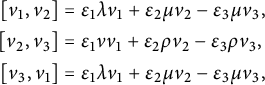 $$ \begin{align*} \left[v_1,v_2\right]&=\varepsilon_{1}\lambda v_1+\varepsilon_2\mu v_2-\varepsilon_3\mu v_3,\\ \left[v_2,v_3\right]&=\varepsilon_{1}\nu v_1+\varepsilon_2\rho v_2-\varepsilon_3\rho v_3,\\ \left[v_3,v_1\right]&=\varepsilon_{1}\lambda v_1+\varepsilon_2\mu v_2-\varepsilon_3\mu v_3, \end{align*} $$
with
 $ \lambda +\rho \neq 0 $
. Using the Dorfman coefficients, that were computed in the proof of Proposition 3.7, we obtain the components of the Ricci tensor
$ \lambda +\rho \neq 0 $
. Using the Dorfman coefficients, that were computed in the proof of Proposition 3.7, we obtain the components of the Ricci tensor
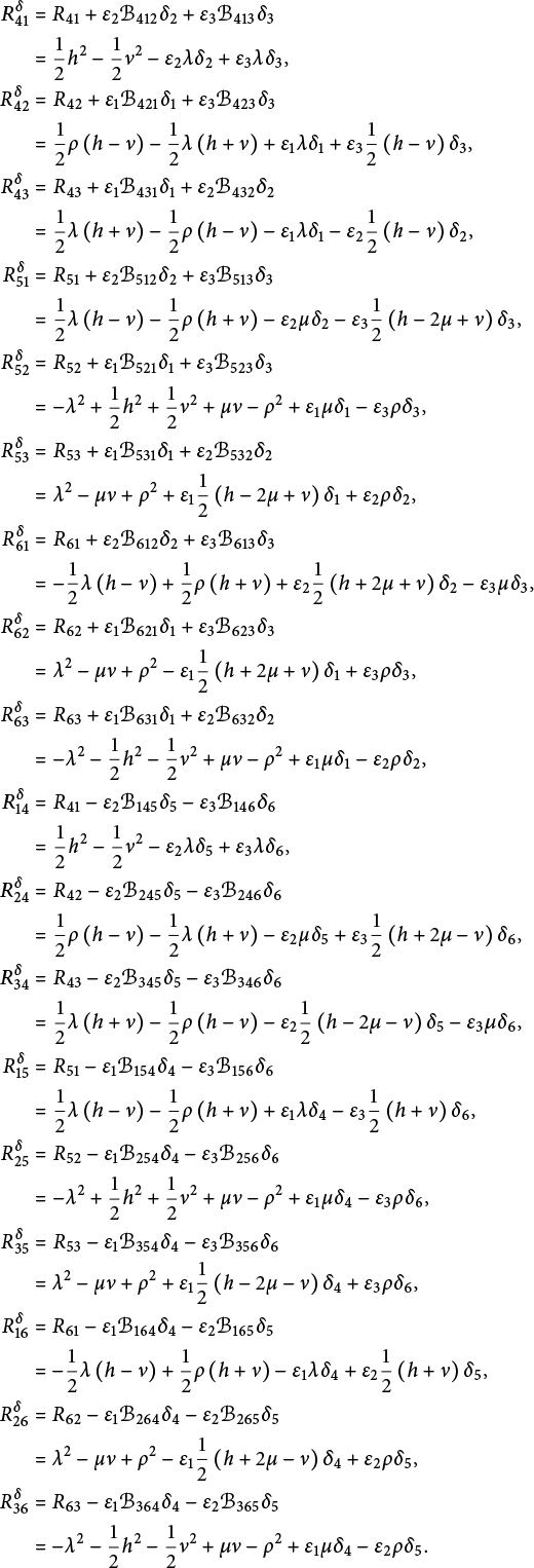 $$ \begin{align*} R_{41}^{\delta}&=R_{41}+\varepsilon_2\mathcal{B}_{412}\delta_2+\varepsilon_3\mathcal{B}_{413}\delta_3\\ &=\frac12h^2-\frac12\nu^2-\varepsilon_2\lambda\delta_2+\varepsilon_3\lambda\delta_3,\\ R_{42}^{\delta}&=R_{42}+\varepsilon_1\mathcal{B}_{421}\delta_1+\varepsilon_3\mathcal{B}_{423}\delta_3\\ &=\frac12\rho\left(h-\nu\right)-\frac12\lambda\left(h+\nu\right)+\varepsilon_1\lambda\delta_1+\varepsilon_3\frac12\left(h-\nu\right)\delta_3,\\ R_{43}^{\delta}&=R_{43}+\varepsilon_1\mathcal{B}_{431}\delta_1+\varepsilon_2\mathcal{B}_{432}\delta_2\\ &=\frac12\lambda\left(h+\nu\right)-\frac12\rho\left(h-\nu\right)-\varepsilon_1\lambda\delta_1-\varepsilon_2\frac12\left(h-\nu\right)\delta_2,\\ R_{51}^{\delta}&=R_{51}+\varepsilon_2\mathcal{B}_{512}\delta_2+\varepsilon_3\mathcal{B}_{513}\delta_3\\ &=\frac12\lambda\left(h-\nu\right)-\frac12\rho\left(h+\nu\right)-\varepsilon_2\mu\delta_2-\varepsilon_3\frac12\left(h-2\mu+\nu\right)\delta_3,\\ R_{52}^{\delta}&=R_{52}+\varepsilon_1\mathcal{B}_{521}\delta_1+\varepsilon_3\mathcal{B}_{523}\delta_3\\ &=-\lambda^2+\frac12h^2+\frac12\nu^2+\mu\nu-\rho^2+\varepsilon_1\mu\delta_1-\varepsilon_3\rho\delta_3,\\ R_{53}^{\delta}&=R_{53}+\varepsilon_1\mathcal{B}_{531}\delta_1+\varepsilon_2\mathcal{B}_{532}\delta_2\\ &=\lambda^2-\mu\nu+\rho^2+\varepsilon_1\frac12\left(h-2\mu+\nu\right)\delta_1+\varepsilon_2\rho\delta_2,\\ R_{61}^{\delta}&=R_{61}+\varepsilon_2\mathcal{B}_{612}\delta_2+\varepsilon_3\mathcal{B}_{613}\delta_3\\ &=-\frac12\lambda\left(h-\nu\right)+\frac12\rho\left(h+\nu\right)+\varepsilon_2\frac12\left(h+2\mu+\nu\right)\delta_2-\varepsilon_3\mu\delta_3,\\ R_{62}^{\delta}&=R_{62}+\varepsilon_1\mathcal{B}_{621}\delta_1+\varepsilon_3\mathcal{B}_{623}\delta_3\\ &=\lambda^2-\mu\nu+\rho^2-\varepsilon_1\frac12\left(h+2\mu+\nu\right)\delta_1+\varepsilon_3\rho\delta_3,\\ R_{63}^{\delta}&=R_{63}+\varepsilon_1\mathcal{B}_{631}\delta_1+\varepsilon_2\mathcal{B}_{632}\delta_2\\ &=-\lambda^2-\frac12h^2-\frac12\nu^2+\mu\nu-\rho^2+\varepsilon_1\mu\delta_1-\varepsilon_2\rho\delta_2,\\ R_{14}^{\delta}&=R_{41}-\varepsilon_2\mathcal{B}_{145}\delta_5-\varepsilon_3\mathcal{B}_{146}\delta_6\\ &=\frac12h^2-\frac12\nu^2-\varepsilon_2\lambda\delta_5+\varepsilon_3\lambda\delta_6,\\ R_{24}^{\delta}&=R_{42}-\varepsilon_2\mathcal{B}_{245}\delta_5-\varepsilon_3\mathcal{B}_{246}\delta_6\\ &=\frac12\rho\left(h-\nu\right)-\frac12\lambda\left(h+\nu\right)-\varepsilon_2\mu\delta_5+\varepsilon_3\frac12\left(h+2\mu-\nu\right)\delta_6,\\ R_{34}^{\delta}&=R_{43}-\varepsilon_2\mathcal{B}_{345}\delta_5-\varepsilon_3\mathcal{B}_{346}\delta_6\\ &=\frac12\lambda\left(h+\nu\right)-\frac12\rho\left(h-\nu\right)-\varepsilon_2\frac12\left(h-2\mu-\nu\right)\delta_5-\varepsilon_3\mu\delta_6,\\ R_{15}^{\delta}&=R_{51}-\varepsilon_1\mathcal{B}_{154}\delta_4-\varepsilon_3\mathcal{B}_{156}\delta_6\\ &=\frac12\lambda\left(h-\nu\right)-\frac12\rho\left(h+\nu\right)+\varepsilon_1\lambda\delta_4-\varepsilon_3\frac12\left(h+\nu\right)\delta_6,\\ R_{25}^{\delta}&=R_{52}-\varepsilon_1\mathcal{B}_{254}\delta_4-\varepsilon_3\mathcal{B}_{256}\delta_6\\ &=-\lambda^2+\frac12h^2+\frac12\nu^2+\mu\nu-\rho^2+\varepsilon_1\mu\delta_4-\varepsilon_3\rho\delta_6,\\ R_{35}^{\delta}&=R_{53}-\varepsilon_1\mathcal{B}_{354}\delta_4-\varepsilon_3\mathcal{B}_{356}\delta_6\\ &=\lambda^2-\mu\nu+\rho^2+\varepsilon_1\frac12\left(h-2\mu-\nu\right)\delta_4+\varepsilon_3\rho\delta_6,\\ R_{16}^{\delta}&=R_{61}-\varepsilon_1\mathcal{B}_{164}\delta_4-\varepsilon_2\mathcal{B}_{165}\delta_5\\ &=-\frac12\lambda\left(h-\nu\right)+\frac12\rho\left(h+\nu\right)-\varepsilon_1\lambda\delta_4+\varepsilon_2\frac12\left(h+\nu\right)\delta_5,\\ R_{26}^{\delta}&=R_{62}-\varepsilon_1\mathcal{B}_{264}\delta_4-\varepsilon_2\mathcal{B}_{265}\delta_5\\ &=\lambda^2-\mu\nu+\rho^2-\varepsilon_1\frac12\left(h+2\mu-\nu\right)\delta_4+\varepsilon_2\rho\delta_5,\\ R_{36}^{\delta}&=R_{63}-\varepsilon_1\mathcal{B}_{364}\delta_4-\varepsilon_2\mathcal{B}_{365}\delta_5\\ &=-\lambda^2-\frac12h^2-\frac12\nu^2+\mu\nu-\rho^2+\varepsilon_1\mu\delta_4-\varepsilon_2\rho\delta_5. \end{align*} $$
Assume now that
 $(H,\mathcal G_g,\delta )$
is generalized Einstein. We first want to show that
$(H,\mathcal G_g,\delta )$
is generalized Einstein. We first want to show that
 $ h=\nu =0 $
and
$ h=\nu =0 $
and
 $ \varepsilon _2\delta _2=\varepsilon _3\delta _3 $
. For this, consider the system of equations
$ \varepsilon _2\delta _2=\varepsilon _3\delta _3 $
. For this, consider the system of equations
 $ 0=R_{42}^{\delta }+R_{43}^{\delta }=-\frac 12\left (h-\nu \right )\left (\varepsilon _2\delta _2-\varepsilon _3\delta _3\right ) $
and
$ 0=R_{42}^{\delta }+R_{43}^{\delta }=-\frac 12\left (h-\nu \right )\left (\varepsilon _2\delta _2-\varepsilon _3\delta _3\right ) $
and
 $ 0=R_{51}^{\delta }+R_{61}^{\delta }=\frac 12\left (h+\nu \right )\left (\varepsilon _2\delta _2-\varepsilon _3\delta _3\right ) $
. This implies that either
$ 0=R_{51}^{\delta }+R_{61}^{\delta }=\frac 12\left (h+\nu \right )\left (\varepsilon _2\delta _2-\varepsilon _3\delta _3\right ) $
. This implies that either
 $ h=\nu =0 $
or
$ h=\nu =0 $
or
 $ \varepsilon _2\delta _2=\varepsilon _3\delta _3 $
. If
$ \varepsilon _2\delta _2=\varepsilon _3\delta _3 $
. If
 $ h=\nu =0 $
, then
$ h=\nu =0 $
, then
 $ 0=R_{41}^{\delta }=-\lambda \left (\varepsilon _2\delta _2-\varepsilon _3\delta _3\right ) $
and
$ 0=R_{41}^{\delta }=-\lambda \left (\varepsilon _2\delta _2-\varepsilon _3\delta _3\right ) $
and
 $ 0=R_{63}^{\delta }-R_{52}^{\delta }=-\rho \left (\varepsilon _2\delta _2-\varepsilon _3\delta _3\right ) $
, which can only be the case if
$ 0=R_{63}^{\delta }-R_{52}^{\delta }=-\rho \left (\varepsilon _2\delta _2-\varepsilon _3\delta _3\right ) $
, which can only be the case if
 $ \varepsilon _2\delta _2=\varepsilon _3\delta _3 $
, since
$ \varepsilon _2\delta _2=\varepsilon _3\delta _3 $
, since
 $ \lambda +\rho \ne 0 $
. If we otherwise assume, that
$ \lambda +\rho \ne 0 $
. If we otherwise assume, that
 $ \varepsilon _2\delta _2=\varepsilon _3\delta _3 $
, then
$ \varepsilon _2\delta _2=\varepsilon _3\delta _3 $
, then
 $ 0=R_{63}^{\delta }-R_{52}^{\delta }=-h^2-\nu ^2 $
and therefore
$ 0=R_{63}^{\delta }-R_{52}^{\delta }=-h^2-\nu ^2 $
and therefore
 $ h=\nu =0 $
. Similarly, one can also show that
$ h=\nu =0 $
. Similarly, one can also show that
 $ \varepsilon _2\delta _5=\varepsilon _3\delta _6 $
. Hence, the Einstein condition is equivalent to the set of equations
$ \varepsilon _2\delta _5=\varepsilon _3\delta _6 $
. Hence, the Einstein condition is equivalent to the set of equations
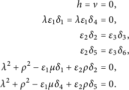 $$ \begin{align} \begin{aligned} h=\nu&=0,\\ \lambda\varepsilon_1\delta_1=\lambda\varepsilon_1\delta_4&=0,\\ \varepsilon_2\delta_2&=\varepsilon_3\delta_3,\\ \varepsilon_2\delta_5&=\varepsilon_3\delta_6,\\ \lambda^2+\rho^2-\varepsilon_1\mu\delta_1+\varepsilon_2\rho\delta_2&=0,\\ \lambda^2+\rho^2-\varepsilon_1\mu\delta_4+\varepsilon_2\rho\delta_5&=0. \end{aligned} \end{align} $$
Now, as in the proof of Proposition 3.7, there exists a basis
 $ (w_a) $
of
$ (w_a) $
of
 $ \mathfrak {g} $
, such that
$ \mathfrak {g} $
, such that
 $ w_1,w_2\in \mathfrak {u} $
,
$ w_1,w_2\in \mathfrak {u} $
,
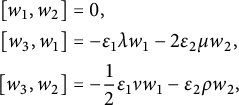 $$ \begin{align*} \left[w_1,w_2\right]&=0,\\ \left[w_3,w_1\right]&=-\varepsilon_1\lambda w_1-2\varepsilon_2\mu w_2,\\ \left[w_3,w_2\right]&=-\frac12\varepsilon_1\nu w_1-\varepsilon_2\rho w_2, \end{align*} $$
and
 $ g(w_a,w_b) $
satisfies equation (28). Hence,
$ g(w_a,w_b) $
satisfies equation (28). Hence,
 $ \mathfrak {g} $
is a semidirect product of
$ \mathfrak {g} $
is a semidirect product of
 $ \mathbb {R}\cong \mathrm {span}\{ w_3\} $
and
$ \mathbb {R}\cong \mathrm {span}\{ w_3\} $
and
 $ \mathbb {R}^2\cong \mathrm {span}\{ w_1,w_2\} $
, the former acting on the latter with the matrix
$ \mathbb {R}^2\cong \mathrm {span}\{ w_1,w_2\} $
, the former acting on the latter with the matrix
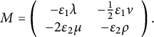 $$ \begin{align*} M=\left( \begin{array}{cc}-\varepsilon_1\lambda& -\frac12\varepsilon_1\nu\\ -2\varepsilon_2\mu & -\varepsilon_2\rho \end{array}\right). \end{align*} $$
Since in the Einstein case
 $ \nu =0 $
, its eigenvalues
$ \nu =0 $
, its eigenvalues
 $ -\varepsilon _1\lambda $
and
$ -\varepsilon _1\lambda $
and
 $ -\varepsilon _2\rho $
are real. Furthermore, for any such matrix, with
$ -\varepsilon _2\rho $
are real. Furthermore, for any such matrix, with
 $ \nu =0 $
, one can find
$ \nu =0 $
, one can find
 $ \delta \in E^* $
, such that
$ \delta \in E^* $
, such that
 $(H=0,\mathcal G_g,\delta )$
is generalized Einstein. In fact, if
$(H=0,\mathcal G_g,\delta )$
is generalized Einstein. In fact, if
 $\lambda \neq 0$
, then
$\lambda \neq 0$
, then
 $h=\nu =\delta _1=\delta _4=0$
,
$h=\nu =\delta _1=\delta _4=0$
,
 $\rho \neq 0$
and the solution is uniquely determined by the free parameters
$\rho \neq 0$
and the solution is uniquely determined by the free parameters
 $\lambda \neq 0, \rho \neq 0$
and
$\lambda \neq 0, \rho \neq 0$
and
 $\mu $
as
$\mu $
as
 $\delta _2=\delta _5=-\delta _3=-\delta _6= -\varepsilon _2 (\lambda ^2 +\rho ^2)/\rho \neq 0$
. If
$\delta _2=\delta _5=-\delta _3=-\delta _6= -\varepsilon _2 (\lambda ^2 +\rho ^2)/\rho \neq 0$
. If
 $\lambda =0$
, then
$\lambda =0$
, then
 $\rho \neq 0$
(as
$\rho \neq 0$
(as
 $\lambda +\rho \neq 0$
),
$\lambda +\rho \neq 0$
),
 $h=\nu = \lambda =0$
and the solution is uniquely determined by the free parameters
$h=\nu = \lambda =0$
and the solution is uniquely determined by the free parameters
 $\mu , \delta _1$
and
$\mu , \delta _1$
and
 $\delta _4$
as
$\delta _4$
as
 $\delta _2= -\delta _3=-\varepsilon _2(\rho ^2-\varepsilon _1\mu \delta _1)/\rho $
and
$\delta _2= -\delta _3=-\varepsilon _2(\rho ^2-\varepsilon _1\mu \delta _1)/\rho $
and
 $\delta _5=-\delta _6=-\varepsilon _2(\rho ^2 -\varepsilon _1\mu \delta _4)/\rho $
. Note that all the solutions have nonzero divergence and that M has rank 1 if and only if
$\delta _5=-\delta _6=-\varepsilon _2(\rho ^2 -\varepsilon _1\mu \delta _4)/\rho $
. Note that all the solutions have nonzero divergence and that M has rank 1 if and only if
 $\lambda =0$
.
$\lambda =0$
.
3.4 Riemannian divergence
In this section, we want to determine those solutions
 $(G,H,\mathcal {G},\delta )$
to the generalized Einstein equation for which the divergence
$(G,H,\mathcal {G},\delta )$
to the generalized Einstein equation for which the divergence
 $ \delta $
coincides with the Riemannian divergence
$ \delta $
coincides with the Riemannian divergence
 $\delta ^{\mathcal {G}} =-\tau \circ \pi \in E^*$
(see Proposition 2.17). If the Lie group is unimodular, the trace-form
$\delta ^{\mathcal {G}} =-\tau \circ \pi \in E^*$
(see Proposition 2.17). If the Lie group is unimodular, the trace-form
 $ \tau $
, and therefore the Riemannian divergence, is zero. This was covered in Theorem 3.4. It remains to specify the results of Propositions 3.15 and 3.16 to the case
$ \tau $
, and therefore the Riemannian divergence, is zero. This was covered in Theorem 3.4. It remains to specify the results of Propositions 3.15 and 3.16 to the case
 $ \delta =\delta ^{\mathcal {G}} $
.
$ \delta =\delta ^{\mathcal {G}} $
.
In the case that
 $ g $
is nondegenerate on the unimodular kernel
$ g $
is nondegenerate on the unimodular kernel
 $ \mathfrak {u} $
,
$ \mathfrak {u} $
,
 $ \delta =\delta ^{\mathcal {G}} $
holds if and only if the components of
$ \delta =\delta ^{\mathcal {G}} $
holds if and only if the components of
 $ \delta $
in the basis
$ \delta $
in the basis
 $ (v_a) $
of
$ (v_a) $
of
 $ \mathfrak {g} $
from Proposition 3.15 are
$ \mathfrak {g} $
from Proposition 3.15 are
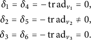 $$ \begin{align*} \begin{aligned} \delta_1=\delta_4=-\operatorname{\mathrm{tr}} \mathrm{ad}_{v_1}&=0,\\ \delta_2=\delta_5=-\operatorname{\mathrm{tr}} \mathrm{ad}_{v_2}&\ne0,\\ \delta_3=\delta_6=-\operatorname{\mathrm{tr}} \mathrm{ad}_{v_3}&=0. \end{aligned} \end{align*} $$
Therefore, the relevant solutions are those for which
 $ M=\mathrm {ad}_{v_2}|_{\mathfrak {u}} $
is diagonalizable and
$ M=\mathrm {ad}_{v_2}|_{\mathfrak {u}} $
is diagonalizable and
 $\delta _1=\delta _3=\delta _4=\delta _6=0$
, in virtue of Proposition 3.15.
$\delta _1=\delta _3=\delta _4=\delta _6=0$
, in virtue of Proposition 3.15.
In the case that
 $ g $
is degenerate on the unimodular kernel
$ g $
is degenerate on the unimodular kernel
 $ \mathfrak {u} $
, we compute the components of
$ \mathfrak {u} $
, we compute the components of
 $ \delta $
in the basis
$ \delta $
in the basis
 $ (v_a) $
of
$ (v_a) $
of
 $ \mathfrak {g} $
from Proposition 3.16 as
$ \mathfrak {g} $
from Proposition 3.16 as
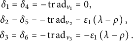 $$ \begin{align*} \begin{aligned} \delta_1=\delta_4=-\operatorname{\mathrm{tr}} \mathrm{ad}_{v_1}&=0,\\ \delta_2=\delta_5=-\operatorname{\mathrm{tr}} \mathrm{ad}_{v_2}&=\varepsilon_1\left(\lambda-\rho\right),\\ \delta_3=\delta_6=-\operatorname{\mathrm{tr}} \mathrm{ad}_{v_3} &=-\varepsilon_1\left(\lambda-\rho\right). \end{aligned} \end{align*} $$
From the system of equation (31), which is equivalent to the Einstein condition, we see now that
 $ \lambda ^2+\lambda \rho =0 $
. Hence,
$ \lambda ^2+\lambda \rho =0 $
. Hence,
 $ \lambda =0 $
, since
$ \lambda =0 $
, since
 $ \lambda +\rho \ne 0 $
. Finally, we conclude that
$ \lambda +\rho \ne 0 $
. Finally, we conclude that
 $ \mathfrak {g}\cong \mathbb {R}\ltimes _A \mathbb {R}^2 $
, where
$ \mathfrak {g}\cong \mathbb {R}\ltimes _A \mathbb {R}^2 $
, where
 $ A $
has one eigenvalue equal to zero and one nonzero eigenvalue.
$ A $
has one eigenvalue equal to zero and one nonzero eigenvalue.
Proposition 3.17 Let
 $(H,\mathcal G_g,\delta )$
be a generalized Einstein structure on a three-dimensional nonunimodular Lie group G, with
$(H,\mathcal G_g,\delta )$
be a generalized Einstein structure on a three-dimensional nonunimodular Lie group G, with
 $ \delta =\delta ^{\mathcal {G}_g} $
the Riemannian divergence of
$ \delta =\delta ^{\mathcal {G}_g} $
the Riemannian divergence of
 $ \mathcal {G}_g $
. Let
$ \mathcal {G}_g $
. Let
 $ \mathfrak {u} $
be the unimodular kernel of the Lie algebra
$ \mathfrak {u} $
be the unimodular kernel of the Lie algebra
 $ \mathfrak {g} $
. If the pseudo-Riemannian metric
$ \mathfrak {g} $
. If the pseudo-Riemannian metric
 $ g $
is nondegenerate on
$ g $
is nondegenerate on
 $ \mathfrak {u} $
, then
$ \mathfrak {u} $
, then
 $\mathfrak {g} \cong \mathbb {R}\ltimes _A \mathbb {R}^2$
for a diagonalizable matrix
$\mathfrak {g} \cong \mathbb {R}\ltimes _A \mathbb {R}^2$
for a diagonalizable matrix
 $ A $
, with
$ A $
, with
 $ \operatorname {\mathrm{tr}} A \ne 0 $
. If
$ \operatorname {\mathrm{tr}} A \ne 0 $
. If
 $ g $
is degenerate on
$ g $
is degenerate on
 $ \mathfrak {u} $
, then
$ \mathfrak {u} $
, then
 $ \mathfrak {g}\cong \mathbb {R}\ltimes _A \mathbb {R}^2 $
for a matrix
$ \mathfrak {g}\cong \mathbb {R}\ltimes _A \mathbb {R}^2 $
for a matrix
 $ A $
, whose kernel is one-dimensional. In both cases, the matrix A can be brought to the form
$ A $
, whose kernel is one-dimensional. In both cases, the matrix A can be brought to the form
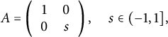 $$\begin{align*}A = \left( \begin{array}{cc}1&0\\ 0&s\end{array}\right), \quad s \in (-1,1],\end{align*}$$
by an automorphism of
 $\mathfrak {g}$
, where
$\mathfrak {g}$
, where
 $s =0$
if
$s =0$
if
 $\mathfrak {u}$
is degenerate. (The precise tensors H,
$\mathfrak {u}$
is degenerate. (The precise tensors H,
 $g,$
and
$g,$
and
 $\delta $
are specified in Propositions 3.15 and 3.16 by specializing to the formulas for
$\delta $
are specified in Propositions 3.15 and 3.16 by specializing to the formulas for
 $\delta =\delta ^{\mathcal {G}_g}$
given in this section.)
$\delta =\delta ^{\mathcal {G}_g}$
given in this section.)
4 Tables
In this section, we want to summarize our results. For further details, we refer to Section 3. In Tables 1 and 2,
 $ L \mathsf{D} $
and
$ L \mathsf{D} $
and
 $ L \neg \mathsf{D} $
mean that the endomorphism
$ L \neg \mathsf{D} $
mean that the endomorphism
 $ L $
defined in equation (23) is diagonalizable and not diagonalizable, respectively. Furthermore, we write def, indef, deg, and nondeg instead of definite, indefinite, degenerate, and nondegenerate. For the notations of the isomorphism classes of Lie algebras, we refer to [Reference Gorbatsevich, Onishchik and VinbergGOV, Chapter 7, Theorem 1.4]. Following [Reference Gorbatsevich, Onishchik and VinbergGOV, Chapter 7, Theorem 1.4], we restrict the parameter
$ L $
defined in equation (23) is diagonalizable and not diagonalizable, respectively. Furthermore, we write def, indef, deg, and nondeg instead of definite, indefinite, degenerate, and nondegenerate. For the notations of the isomorphism classes of Lie algebras, we refer to [Reference Gorbatsevich, Onishchik and VinbergGOV, Chapter 7, Theorem 1.4]. Following [Reference Gorbatsevich, Onishchik and VinbergGOV, Chapter 7, Theorem 1.4], we restrict the parameter
 $\lambda $
in
$\lambda $
in
 $\mathfrak {r}_{3,\lambda }(\mathbb {R})$
to
$\mathfrak {r}_{3,\lambda }(\mathbb {R})$
to
 $0<|\lambda | \le 1$
. In addition, we exclude
$0<|\lambda | \le 1$
. In addition, we exclude
 $\lambda =-1$
, since
$\lambda =-1$
, since
 $\mathfrak {r}_{3,-1}(\mathbb {R})\cong \mathfrak {e}(1,1)$
.
$\mathfrak {r}_{3,-1}(\mathbb {R})\cong \mathfrak {e}(1,1)$
.
Table 1. Divergence-free solutions to the generalized Einstein equation.
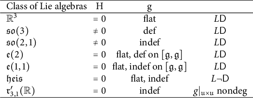
Table 2. Solutions to the generalized Einstein equation with arbitrary divergence.

Acknowledgment
We thank Liana David, Mario García Fernández, and Carlos Shahbazi for helpful comments.


 Open access