the Creative Commons Attribution 4.0 License.
the Creative Commons Attribution 4.0 License.
 | 06 Jul 2021
Identifying the sources of uncertainty in climate model simulations of solar radiation modification with the G6sulfur and G6solar Geoengineering Model Intercomparison Project (GeoMIP) simulations
Daniele Visioni
Douglas G. MacMartin
Ben Kravitz
Olivier Boucher
Andy Jones
Thibaut Lurton
Michou Martine
Michael J. Mills
Pierre Nabat
Ulrike Niemeier
Roland Séférian
Simone Tilmes
We present here results from the Geoengineering Model Intercomparison Project (GeoMIP) simulations for the experiments G6sulfur and G6solar for six Earth system models participating in the Climate Model Intercomparison Project (CMIP) Phase 6. The aim of the experiments is to reduce the warming that results from a high-tier emission scenario (Shared Socioeconomic Pathways SSP5-8.5) to that resulting from a medium-tier emission scenario (SSP2-4.5). These simulations aim to analyze the response of climate models to a reduction in incoming surface radiation as a means to reduce global surface temperatures, and they do so either by simulating a stratospheric sulfate aerosol layer or, in a more idealized way, through a uniform reduction in the solar constant in the model. We find that over the final two decades of this century there are considerable inter-model spreads in the needed injection amounts of sulfate (29 ± 9 Tg-SO2/yr between 2081 and 2100), in the latitudinal distribution of the aerosol cloud and in the stratospheric temperature changes resulting from the added aerosol layer. Even in the simpler G6solar experiment, there is a spread in the needed solar dimming to achieve the same global temperature target (1.91 ± 0.44 %). The analyzed models already show significant differences in the response to the increasing CO2 concentrations for global mean temperatures and global mean precipitation (2.05 K ± 0.42 K and 2.28 ± 0.80 %, respectively, for SSP5-8.5 minus SSP2-4.5 averaged over 2081–2100). With aerosol injection, the differences in how the aerosols spread further change some of the underlying uncertainties, such as the global mean precipitation response (−3.79 ± 0.76 % for G6sulfur compared to −2.07 ± 0.40 % for G6solar against SSP2-4.5 between 2081 and 2100). These differences in the behavior of the aerosols also result in a larger uncertainty in the regional surface temperature response among models in the case of the G6sulfur simulations, suggesting the need to devise various, more specific experiments to single out and resolve particular sources of uncertainty. The spread in the modeled response suggests that a degree of caution is necessary when using these results for assessing specific impacts of geoengineering in various aspects of the Earth system. However, all models agree that compared to a scenario with unmitigated warming, stratospheric aerosol geoengineering has the potential to both globally and locally reduce the increase in surface temperatures.
- Article
(30448 KB) -
Supplement
(327 KB) - BibTeX
- EndNote


Solar radiation modification (SRM) is defined as the proposed artificial altering of the radiative balance of the planet in order to temporarily counteract some of the imbalance produced by the increase in atmospheric greenhouse gases (GHGs). This might be achieved in multiple ways, but the most studied one, originally proposed by Budyko (1977) and Crutzen (2006), would consist of the injection of SO2 into the stratosphere in order to produce a layer of sulfate aerosols capable of partially reflecting incoming solar radiation; this is usually defined as stratospheric aerosol intervention (SAI) or sulfate geoengineering. Simulating such a technique in climate models is the main way to understand the possible impacts on the composition of the atmosphere and on the surface climate to determine its eventual feasibility, understand its possible impacts on ecosystems and populations (Zarnetske et al., 2021) and inform policymakers and stakeholders.
The Geoengineering Model Intercomparison Project (GeoMIP) was proposed initially in Kravitz et al. (2011) as a way to standardize SRM modeling experiments, allowing for a more robust comparison between model responses and determination of sources of uncertainties and areas for improvement. Whereas the term “geoengineering”, “climate engineering” or, more recently, “climate intervention” (https://www.silverlining.ngo/us-national-survey-terminology-for-approaches-for-directly-influencing-climate, last access: 28 June 2021) are also usually used to consider methods of carbon dioxide removal (CDR), in the original intention of GeoMIP (and this work) it was only considered as a more colloquial term for SRM.
Two previous experiments in particular have been widely analyzed and discussed: G1, where the solar constant is reduced in order to offset the temperature increase produced by a 4× increase in CO2 compared to pre-industrial concentrations (Kravitz et al., 2013b; Tilmes et al., 2013; Glienke et al., 2015; Russotto and Ackerman, 2018b; Kravitz et al., 2021), and G4, where a constant amount of SO2 is injected into the equatorial stratosphere under emissions from the Representative Concentration Pathway 4.5 (RCP4.5) (Pitari et al., 2014; Kashimura et al., 2017; Visioni et al., 2017b; Plazzotta et al., 2019. However, previously performed GeoMIP experiments were not intended to be “realistic” deployments of geoengineering, either because they were performed under idealized conditions (such as 4×CO2 concentrations) or because they considered a fixed, constant amount of injected SO2 with an abrupt beginning and ending. Furthermore, in the case of the G4 experiment, there was no scenario to compare in which similar global mean temperatures were achieved with lower CO2 but no geoengineering. Two new experiments have been proposed as part of the GeoMIP Phase 6 (Kravitz et al., 2013b) where geoengineering is aimed at lowering global mean surface temperatures from those in a high-tier emission scenario (Shared Socioeconomic Pathway; SSP5-8.5; Meinshausen et al., 2020) to those in a medium-tier emission scenario (SSP2-4.5). G6sulfur aims to achieve this temperature goal by increasing the simulated stratospheric aerosol optical depth (AOD). In models with an interactive sulfur cycle and stratospheric aerosol microphysics this is done by simulating the injection of SO2 between 10∘ N and 10∘ S between 18 and 20 km, whereas in other models this is done by imposing a sulfate distribution calculated offline. G6solar, on the other hand, decreases total incoming solar irradiance. While the latter does not aim to reproduce the effects of an actual sulfate aerosol intervention, comparisons of its results with simulations of stratospheric aerosols in the same model may help understand the contributions to inter-model differences in the response to aerosols (Niemeier et al., 2013; Visioni et al., 2021). Both reductions of incoming solar radiation at the surface (directly, by turning down the Sun, or indirectly, by having the aerosols reflect the solar radiation) are adjusted at least every decade to ensure that the target temperature is being met.
There are multiple uncertainties that can be investigated with a multi-model intercomparison when considering the climate models' responses to an artificial, deliberate modification of surface temperatures by means of stratospheric aerosols (Kravitz and MacMartin, 2020). In the stratosphere, these include the conversion of injected SO2 into stratospheric aerosol and the subsequent large-scale distribution of the aerosols by stratospheric circulation (not dissimilar to multi-model analyses of simulations of explosive volcanic eruptions; Marshall et al., 2018; Clyne et al., 2021), the chemical response of key stratospheric components (ozone, methane) to the aerosol layer (Pitari et al., 2014; Visioni et al., 2017b), the magnitude of the produced local heating (Niemeier et al., 2020) and the dynamical response. At the surface, uncertainties include the magnitude of the resulting global cooling per Tg-SO2 injected or per unit of optical depth produced, the regional patterns of change in temperature (Kravitz et al., 2013a), precipitation (Kravitz et al., 2013b; Tilmes et al., 2013) and extreme events (Aswathy et al., 2015; Ji et al., 2018) as well as other variables that might affect ecosystems and populations (Zarnetske et al., 2021), such as tropospheric ozone (Xia et al., 2017) or cloud changes (Russotto and Ackerman, 2018a).
In this work we analyze the response to the two proposed experiments in six global climate models, all part of the Climate Model Intercomparison Project, Phase 6 (CMIP6), in order to explore some of the described uncertainties in these state-of-the-art models. After briefly describing the participating models and the experimental setups in Sect. 3.1, we first confirm that all models successfully manage to lower globally averaged surface temperatures from those of the underlying high emission scenario to those of the medium one. While in the case of a broad solar reduction there is no constraint on the maximum achievable cooling, previous work has suggested a non-linear behavior between injected SO2 and aerosol burden at high amounts of injections (Pierce et al., 2010; Niemeier and Timmreck, 2015), resulting in a reduced efficiency. Therefore we also try to evaluate the presence of a similar non-linearity in the participating models (if it occurs in the range of forcing needed in our experiment). We then analyze in Sect. 3.2 the differences in the latitudinal spread of the stratospheric aerosols cloud despite the consistent injection location. Even when pursuing the same global mean temperature-oriented goal, it has been shown in simulations with CESM1(WACCM) that differences in the latitudinal (Kravitz et al., 2019 and seasonal (Visioni et al., 2020b) distribution of the aerosols can result in significant differences in surface climate. If different models simulate different distributions of the aerosols (as for the G4 experiment; Pitari et al., 2014) due to different stratospheric processes (both dynamical and chemical; Niemeier et al., 2020; Franke et al., 2021), the simulated surface climate would also be different. Furthermore, even given similar simulated aerosol distribution, the stratospheric response might differ due to differences in aerosol optics and in the radiative transfer calculation and in the representation of chemical processes in the stratosphere (i.e., if interactive chemistry is considered in the stratosphere; Franke et al., 2021) resulting in a different dynamical and ultimately surface response (Simpson et al., 2019; Jiang et al., 2019; Banerjee et al., 2021), which we discuss in Sect. 3.3 for annual mean temperature and precipitation.
We analyze four sets of simulations from 2020 to 2100: two baseline scenarios without geoengineering that follow two Shared Socioeconomic Pathways, SSP2-4.5 and SSP5-8.5 (O'Neill et al., 2016), and two scenarios with geoengineering, G6solar and G6sulfur (Kravitz et al., 2015). Overall, six models participated in all experiments (Table 1).
In the SSP2-4.5 and SSP5-8.5, GHG emissions follow a medium and high trajectory, respectively, resulting by the end of the century in a radiative forcing indicated by the last two numbers in the name (i.e., 4.5 and 8.5 W/m2, similar to the Representative Concentration Pathways in CMIP5). The G6 simulations start in 2020 with the same emissions as SSP5-8.5 and, on top of that, have either the solar constant reduced by a certain fraction or produce a sulfate aerosol optical depth with the aim of reducing the globally averaged surface temperature down to the SSP2-4.5 level. While the solar reduction is performed in the same way in all G6solar experiments, reducing the solar constant uniformly at all latitudes, not all participating models included stratospheric aerosols by directly injecting SO2. Two models (IPSL-CM6A-LR and UKESM1-0-LL) injected SO2 uniformly between 10∘ N and 10∘ S between 18 and 20 km of altitude and across a single longitudinal band (∘ 0). CESM2(WACCM) injected SO2 at the Equator and at 25 km of altitude. The others prescribed an already-calculated aerosol optical depth distribution: CNRM-ESM2-1 used an input dataset provided by GeoMIP (the aerosol distribution the G4SSA experiment; Tilmes et al., 2015), while MPI-ESM prescribed their own aerosol distribution derived from the simulations described in Niemeier and Schmidt (2017) and Niemeier et al. (2020). In both cases, the prescribed aerosols are fully integrated in the radiative transfer calculations. Therefore, the response of direct and diffuse radiation at the surface and the localized stratospheric warming due to radiative heating are fully consistent with those from the other models where the full aerosol production from SO2 is simulated (see, for instance, Laakso et al., 2020). However, previous studies have shown the presence of non-linearities at higher injection loads. These can be microphysical in nature, with aerosol particles growing to larger sizes with larger loads of SO2 (Niemeier and Timmreck, 2015), or dynamical, with the stratospheric heating producing changes in stratospheric circulation resulting in a different aerosol distribution in the tropics (Visioni et al., 2018b) or at high latitudes (Visioni et al., 2020a). If the same aerosol distribution is simply scaled up, these effect would not be present in those models.
A summary of the participating models, ensemble size and notes related to the implementation of G6sulfur is provided in Table 1. Further information on the models' components can be found in the references provided for each model and a summary is given in Table S1 in the Supplement. More detailed information for CMIP6 models can also be found in Séférian et al. (2020) for marine biogeochemistry, Arora et al. (2020) for carbon-climate feedbacks and Thornhill et al. (2021) for atmospheric chemistry.
Danabasoglu et al. (2020)Danabasoglu (2019)Gettelman et al. (2019)Séférian et al. (2019)Seferian (2018)Tilmes et al. (2015)Michou et al. (2020)Boucher et al. (2020)Boucher et al. (2018)Lurton et al. (2020)Muller et al. (2018)Wieners et al. (2019)Niemeier and Schmidt (2017)Muller et al. (2018)Jungclaus et al. (2019)Niemeier and Schmidt (2017)Sellar et al. (2019)Tang et al. (2019)Table 1Summary of model simulations used in this work. The first column has the name of the model used, the DOI for the relative CMIP6 dataset as recommended by CMIP6 (see Stockhause and Lautenschlager, 2021) and the horizontal and vertical resolution; the second column indicates the main scientific reference(s) where the model version is described. Columns 3 to 6 show the size of the ensemble analyzed in this work. For some models, more ensemble members are available for the SSP experiments, but only those with the same variant as the G6 experiments are used in this work. Finally, the last two columns indicate the source of stratospheric aerosols for G6 and the presence of interactive stratospheric ozone. All models have interactive marine biogeochemistry and are coupled to an interactive land model.

a Resolution is described as horizontal (h), lat × long, and vertical (v). b Injected at the Equator at 25 km in deviation from the protocol described by Kravitz et al. (2015).
Two modeling teams, IPSL-CM6A-LR and UKESM1-0-LL, determined for every decade by how much to reduce the solar constant or how much more SO2 or prescribed aerosols to have in the stratosphere in order to reduce surface temperatures of the forthcoming decade to SSP2-4.5 levels, whereas four teams, CESM2(WACCM), MPI-ESM1.2-LR, MPI-ESM1.2-HR and CNRM-ESM2-1, did so every year. For CESM2(WACCM), the determination of injected SO2 or reduction of the solar constant is done by a feedback algorithm described in Kravitz et al. (2017) and also used in Tilmes et al. (2018a, 2020).
3.1 Magnitude of geoengineering required
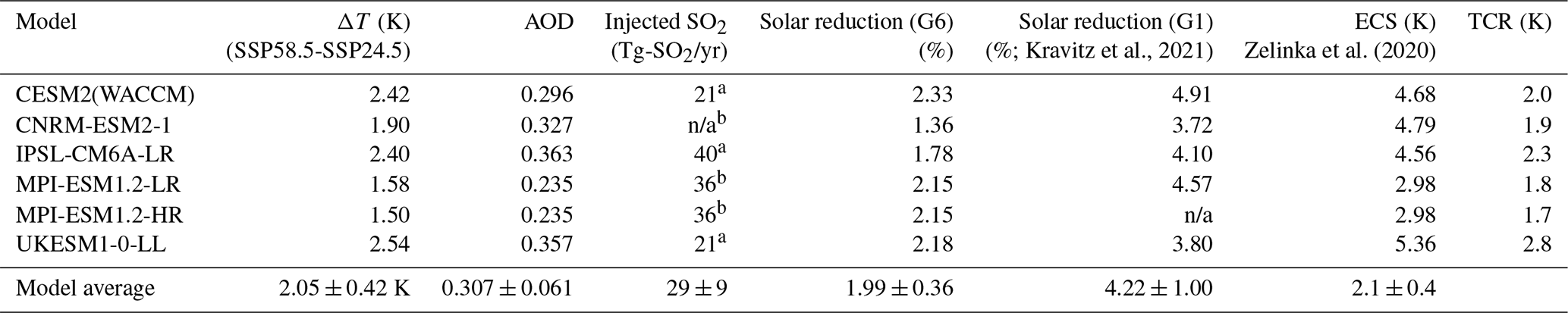
All models successfully reduce global mean surface air temperatures to within 0.2 ∘C of SSP2-4.5 levels on average throughout the century with both geoengineering methods (Fig. 1), but the amount of geoengineering required to do so varies across models. There are a variety of overlapping mechanisms that contribute to these differences. As reported in Table 2, the models produce a large spread in the projected warming produced by the two scenarios. Similar inter-model spreads have been reported in the recent literature for CMIP6 models for both effective equilibrium climate sensitivity (ECS; the equilibrium warming for a doubling of CO2; see Zelinka et al., 2020) and transient climate response (TCR; the temperature warming with a doubling of CO2 in a scenario with a 1 % per year CO2 increase; see Meehl et al., 2020). Some models (amongst them CESM2(WACCM) and UKESM1-0-LL, also present in this study) have been found to have values well above previously established likely ranges for both ECS and TCR (Gettelman et al., 2019; Sherwood et al., 2020). Some of the relationships between the variables reported in Table 2 are explored in Fig. 2. A weak relationship between the different warming in the SSP scenarios and ECS and TCR is to be expected due to differences in both the timescale of the response and the differences in, for instance, other GHGs and tropospheric aerosols (Hansen et al., 2005) that affect the climate in the short term and that are not factored in the long-term response to CO2 changes. For instance, CNRM-ESM2-1 reported an ECS of 4.79 K (Zelinka et al., 2020) (the second highest here) but a ΔT of 1.9 K (the third lowest).

Figure 1Global mean surface temperatures (∘C) for the four experiments for each participating model. Single ensemble realizations are shown in lighter lines, while the ensemble mean is shown in thicker lines. The multi-models mean is shown at the bottom, with the shading representing 1σ standard deviation of the mean for each experiment.
Table 2Summary of results for the simulations in this work for the last two decades of the experiment (2081–2100). When applicable, values are considered as a global mean, ensemble mean averages. In the last three columns, the solar reduction needed in the G1 experiment (Kravitz et al., 2021) to offset the forcing of a 4× CO2 increase, the effective equilibrium climate sensitivity (ECS) from Zelinka et al. (2020) and the transient climate response (TCR) from Meehl et al. (2020) are included for comparison.
a Models using emissions of SO2. b Models using prescribed AOD. n/a – not applicable
This implies that even if different models agreed on how much either stratospheric AOD or reduction of the solar constant would be needed to cool globally by 1 K (the efficacy of the geoengineering method), the overall reported amount of intervention needed would be different due to the different response to the forcing from CO2. To first order, there should be no expectation that the sensitivity of climate models to a CO2 increase should be related to the reduction in temperature due to geoengineering (Kravitz et al., 2021), and we indeed show this in Fig. 2. In Fig. 2f we show that normalizing the required solar dimming or produced AOD in the last two decades to the global cooling in the same period slightly increases the inter-model spread from 19.9 % to 22.8 % for solar dimming and from 17.2 % to 20.7 % for AOD compared to the mean (the same quantities, not normalized, are shown in Fig. S1 in the Supplement). In Fig. 2e we also show that the amount of solar reduction and the globally averaged stratospheric AOD seem to be only weakly related (R2=0.72), suggesting that there are different mechanisms involved in the cooling due to the aerosols and the cooling due to reduced insolation. For G6sulfur, this might be due not only to the radiative treatment of the aerosols themselves but also to different latitudinal distribution in AOD resulting in different forcing compared to the broad solar reduction that is nearly spatially identical in all models.
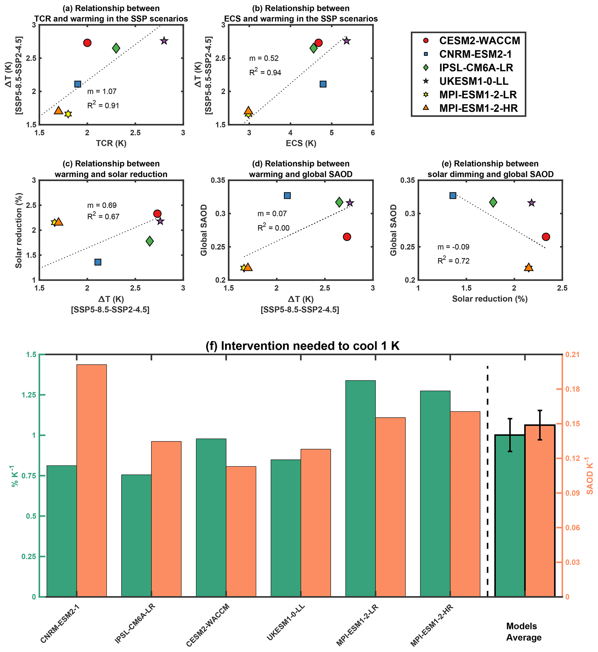
Figure 2(a–e) Scatter plot of various relationships between some global quantities in the participating models. ΔT is between SSP5-8.5 and SSP2-4.5, and global stratospheric aerosol optical depth (SAOD) and solar reduction are defined in the 2081–2100 period. Transient climate response (TCR) and effective equilibrium climate sensitivity (ECS) are taken from Zelinka et al. (2020) and Meehl et al. (2020). The R2 and the slope of the linear fit (m) are shown for each panel. (f) Values in panels (c)–(d) are normalized by the ΔT in the same model to obtain the normalized intervention (green for solar dimming and orange for stratospheric AOD) needed to cool by 1 K, with multi-model average on the right and error bars indicating the standard error.
The time-dependent amount of geoengineering needed in all models for the two experiments is reported in Fig. 3a–b, together with the top-of-atmosphere (TOA) forcing imbalance between SSP5-8.5 and SSP2-4.5, calculated as the incoming minus the outgoing longwave and shortwave radiation (Fig. 3c), and the underlying difference in CO2 concentration, common to all models, as prescribed for the SSP scenarios in Meinshausen et al. (2020) (Fig. 3d). In terms of TOA forcing, models show a more consistent forcing that is a result, mostly, of the same CO2 increase, but they disagree both in the magnitude of the warming produced by this same forcing (as shown in Fig. 1) and in the amount of intervention (optical depth or solar reduction) needed to overcome that forcing, as shown in Fig. 3a and b. The comparison between the two forcings is also useful to understand the behavior of the geoengineering amount in the models in the first 30 years, where most models indicate little to no geoengineering is necessary. CESM2-WACCM is an exception, and indeed shows a slight overcooling in the first decades compared to other models; this is most likely a feature of the current feedback controller, as has been observed in Tilmes et al. (2018a). The algorithm, which decides how much to inject each year by learning from past years, requires some time to properly converge before it can successfully determine the necessary amount. More generally, the small differences between the two underlying scenarios in terms of global mean temperature in the first three decades tend to magnify small differences in the required intervention, as manually estimated by the modeling teams, resulting in larger differences in the first years. Later in the century, when the temperature difference is larger and the intervention scales up, inter-model differences may be explained by the presence of non-linearities or other effects (such as an increase in stratospheric water vapor; Visioni et al., 2017a). It is interesting to note that while a large portion of the models do not vary the amount of geoengineering smoothly, but once a decade, the applied step function is not evident in the globally averaged surface temperature responses shown in Fig. 1, where there is no qualitative difference between models in terms of decadal variability. Since it is similarly present in the G6solar experiments, the reason for this may be found in the slower oceanic response. Future analyses should investigate whether the step function introduced by some of the models results in changes in surface climate that, while hidden when considering global or decadal averages, might be present when looking at particular regions or climate features (for instance, the monsoon season) in the years where the step change is present.
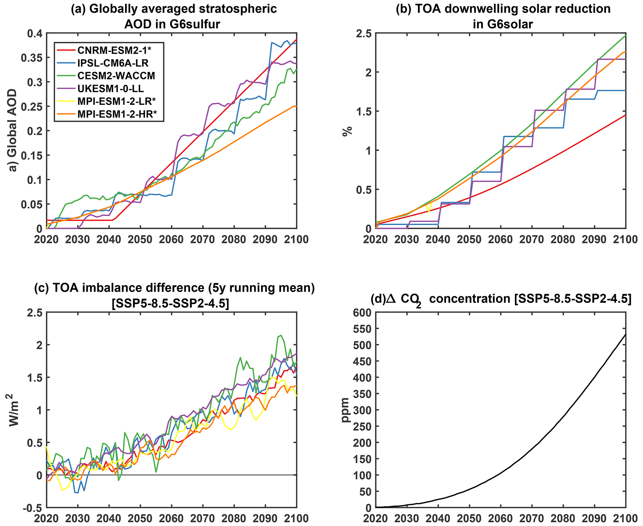
Figure 3Time-dependent evolution for all participating models of (a) globally averaged stratospheric AOD increase in the G6sulfur experiment (models with an asterisk in the legend have prescribed AOD and the orange and yellow line for the two MPI-ESM1-2 versions completely overlap); (b) solar reduction in the G6solar experiment as a fraction of the overall incoming solar radiation; (c) top-of-atmosphere radiative forcing imbalance (downwelling solar radiation minus upwelling solar+longwave radiation) difference between the two baseline SSP scenarios; and (d) difference in CO2 concentration between the two emission scenarios from Meinshausen et al. (2020) presented for reference.
3.2 Differences in the stratospheric response
For the G6sulfur simulations, the global mean AOD is not, on its own, enough to understand the different models' behavior. Different spatial distributions of the aerosol layer, while yielding similar global values, might result in different efficiency and would produce different responses of the surface climate (MacMartin et al., 2017; Kravitz et al., 2019; Visioni et al., 2020b). Reasons for a different aerosol distribution with similar injection locations and height of SO2 can be the different dynamical features of the simulated stratosphere and/or differences in the aerosol microphysics schemes (Pitari et al., 2014; Niemeier et al., 2020; Franke et al., 2021) resulting in different aerosol growth, transport and sedimentation, as already shown for simulations of explosive volcanic eruptions (Marshall et al., 2018; Clyne et al., 2021). The response to the presence of the aerosols themselves can in turn produce differences in stratospheric dynamics, for instance, interacting with the quasi-biennial oscillation (Aquila et al., 2014; Richter et al., 2017), strengthening the tropical confinement of the aerosols (Niemeier and Schmidt, 2017; Visioni et al., 2018b).
Furthermore, even given similar annually averaged AOD distributions, differences in the seasonal cycle might lead to different surface climate (Visioni et al., 2020b). The spatial distributions of AOD for the last decade of the experiment in each model are shown in Fig. 4a. Results vary widely between models: UKESM1-0-LL represents a clear outlier in the tropics, with more than twice the sulfate AOD as other models. At high latitudes, on the other hand, there is a much larger inter-model spread, with values ranging from 0.1 to 0.3 at 90∘ S and from 0.2 to 0.45 at 90∘ N. Strong disagreement between model-simulated AOD in a geoengineering scenario was already reported in Pitari et al. (2014) and Plazzotta et al. (2018) for the G4 experiments, where a 5 Tg-SO2/yr injection in the equatorial stratosphere was prescribed in the simulation protocols. No models used in that experiment have been used in the G6 scenarios, so a direct comparison can't be done with different versions of the same models. In this case, however, we can note that all models at least agree on the presence of a confinement of a portion of the aerosols in the tropical pipe, whereas in G4 half of the models reported much less AOD in the tropics and more at very high latitudes (Pitari et al., 2014), which is physically very unlikely given observations from the Pinatubo eruption in 1991 (Robock, 2000; Pitari et al., 2016).
Model spread on a particular result is not, of course, the same as uncertainty; models may agree despite a lack of observational support, resulting in a narrow spread that might be inaccurate, or the spread might be large because some model results are simply inconsistent with available observations. Here, we try to better constrain the distribution of AOD in the various models in G6sulfur using the up-to-date CMIP6 dataset for volcanic forcing that combines measurements from various sources (Dhomse et al., 2020; retrieved from ftp://iacftp.ethz.ch/pub_read/luo/CMIP6/, last access: 29 October 2020). In particular, using the 550 nm extinction data, we derive the stratosphere-only latitudinal distribution of the optical depth following the Pinatubo 1991 eruption, averaged from 1 month after the eruption (July 1991) to 1 year after in order to also consider the poleward transport of the aerosols. It needs to be highlighted that the comparison between an impulsive injection (as Pinatubo) versus a sustained injection (as in the geoengineering experiment) is an imperfect one, both in terms of the aerosol distribution and in terms of the effects on surface climate (Duan et al., 2019), but it is possibly the only “real”, albeit imperfect, point of comparison between model behavior and the actual atmospheric behavior. In the case of a volcanic eruption, the precise meteorological conditions strongly influence the resulting AOD; furthermore, the SO2 is injected in a clean stratosphere. Therefore, the following comparison should not be considered as a way of measuring which model is closer to observations but just as a way to compare the different models when they reach a similar global AOD. In Fig. 4c we report the AOD from Pinatubo derived this way and we then compare the results with those from the various G6sulfur models. To do so, we consider the year in which each model reaches the same global value of AOD as Pinatubo and plot the latitudinal distribution of AOD for each model in that year. This comparison highlights various elements that would be lost considering the results towards the end of the century as in Fig. 4a. Models show a higher agreement considering a moderate level of global AOD reached and, compared with the results from Pinatubo (considering the differences in meteorology and injection location), they look reasonable. In particular, UKESM1-0-LL and CESM2-WACCM show a better agreement in their tropical AOD, as opposed to what was shown in Fig. 4a, indicating the presence of non-linearities at high injection rates that might be induced in UKESM1-0-LL by a too strong confinement of the aerosols in the tropical pipe as a consequence of the dynamic response to heating (Aquila et al., 2014; Niemeier and Schmidt, 2017; Visioni et al., 2018b). In Fig. 4c, models also show a much better agreement at high latitudes (at least in the Northern Hemisphere) compared to Fig. 4a, with the exception of the prescribed AOD in CNRM-ESM2-1. This suggests that when considering higher injection loads, there could be a stronger interaction of the produced dynamical changes with the simulated AOD at high latitudes (Visioni et al., 2020a).
The amount of SO2 needed to reach a certain stratospheric AOD varies considerably between climate models with interactive stratospheric aerosols even for simulations of Pinatubo, ranging in current estimates between 10 and 20 Tg-SO2 with a central value of 14 (Timmreck et al., 2018). In the G6sulfur experiments, the models show discrepancies in the estimate of the amount needed to achieve a similar global AOD as in Pinatubo (with a multi-model average of 9.3 ± 2.3 Tg-SO2; see table in Fig. 4), closer to the lower limit from Timmreck et al. (2018) (10 Tg-SO2) for UKESM1-0-LL and IPSL-CM6A-LR and 60 % lower for CESM2-WACCM. For CESM2-WACCM, the difference could be partially explained by the difference in altitude for the SO2 injections. In Fig. 4c we also report the cooling produced by the G6sulfur aerosols, compared to SSP5-8.5 in the considered year (we used a 5-year average around that year to reduce the contribution of natural variability). For Pinatubo, there is uncertainty in the cooling produced by the volcanic aerosols due to the precise meteorology of that year (for instance, the influence of an El-Niño event or other climatic oscillations compared to the years immediately before/after); Parker et al. (1996) estimate a global cooling of around 0.4 K, and similarly Soden et al. (2002) estimated a range between 0.3 and 0.5 K, whereas more recent estimates by Canty et al. (2013) found a cooling of 0.14 K when considering the Atlantic multidecadal variability. The multi-model average for the G6sulfur simulation is very similar to the higher estimates, at 0.46 K ± 0.09, but there is a large range in the single values from 0.24 (in MPI-ESM1-2-LR) to 0.74 (for CESM2-WACCM). The two global coolings could be hard to compare, however, due to their different nature (impulsive versus sustained). Overall, the comparisons shown in Fig. 4 raise an important point that should be taken into account when analyzing G6 simulations in future work. While limiting the analyses towards the end of the century might yield a higher signal-to-noise ratio, it also risks magnifying uncertainties related to non-linear processes in the stratosphere. In Fig. S2 in the Supplement, we also report the yearly evolution of the latitudinal distribution of AOD for models that inject SO2, normalized by the amount of SO2 injected in that year, which clearly shows the decrease in efficiency at higher injection loads.
Figure 4(a) Stratospheric AOD in the last decade of the experiment for all participating models. The asterisk in the legend indicates models with prescribed optical depth. (b) Injected SO2 for available models in Tg-SO2/yr. (c) AOD distribution for each model in the year with a global AOD closest to that from Pinatubo (0.102, averaged from July 1991 to June 1992) and comparison with the latitudinal distribution for the volcanic eruption following the new CMIP6 composed dataset (Dhomse et al., 2020). (d) The year where the global value of AOD reaches 0.102 in the model is indicated, together with the amount of SO2 needed to achieve that value and the cooling produced in G6sulfur compared to SSP5-8.5 in that year. Models marked with an asterisk in the legend used prescribed aerosol distributions for G6sulfur. The orange and yellow lines for the two MPI-ESM1-2 versions always overlap.
As mentioned before, the presence of aerosols in the stratosphere also produces a perturbation of stratospheric dynamics (Richter et al., 2017; Visioni et al., 2020a) that, in turn, might affect precipitation (Simpson et al., 2019) and temperature (Jiang et al., 2019) at the surface. The response is driven by the absorption of infrared radiation by the aerosols resulting in the heating of the stratospheric air and is thus dependent on the overall burden and the size of the particles (Pitari et al., 2016) but also on interactions with the chemical cycles in the stratosphere (Visioni et al., 2017b; Richter et al., 2017) and the incursion of water vapor from the troposphere due to the warming of the tropopause layer (Visioni et al., 2017b; Tilmes et al., 2018b; Boucher et al., 2017). In Fig. 5 we show the stratospheric temperatures in the last two decades of the G6sulfur experiment for all models. Interestingly, the model with the highest AOD in the tropics, UKESM1-0-LL, is also one of the models showing the least amount of stratospheric heating, whereas IPSL-CM6A-LR, with an average tropical AOD (but much larger SO2 injection needed to achieve it) shows a temperature change that is much larger than the others. The reasons for this may depend on multiple aspects that would need to be investigated separately. For instance, the reasons might include that there are different size distributions of the stratospheric aerosols, different concentrations of particles (shown in Fig. 5), differences in ozone changes resulting in different heating rates (Richter et al., 2017; Niemeier et al., 2020), different heating from stratospheric water vapor (Pitari et al., 2014; Simpson et al., 2019) or differences in the radiative schemes between models.
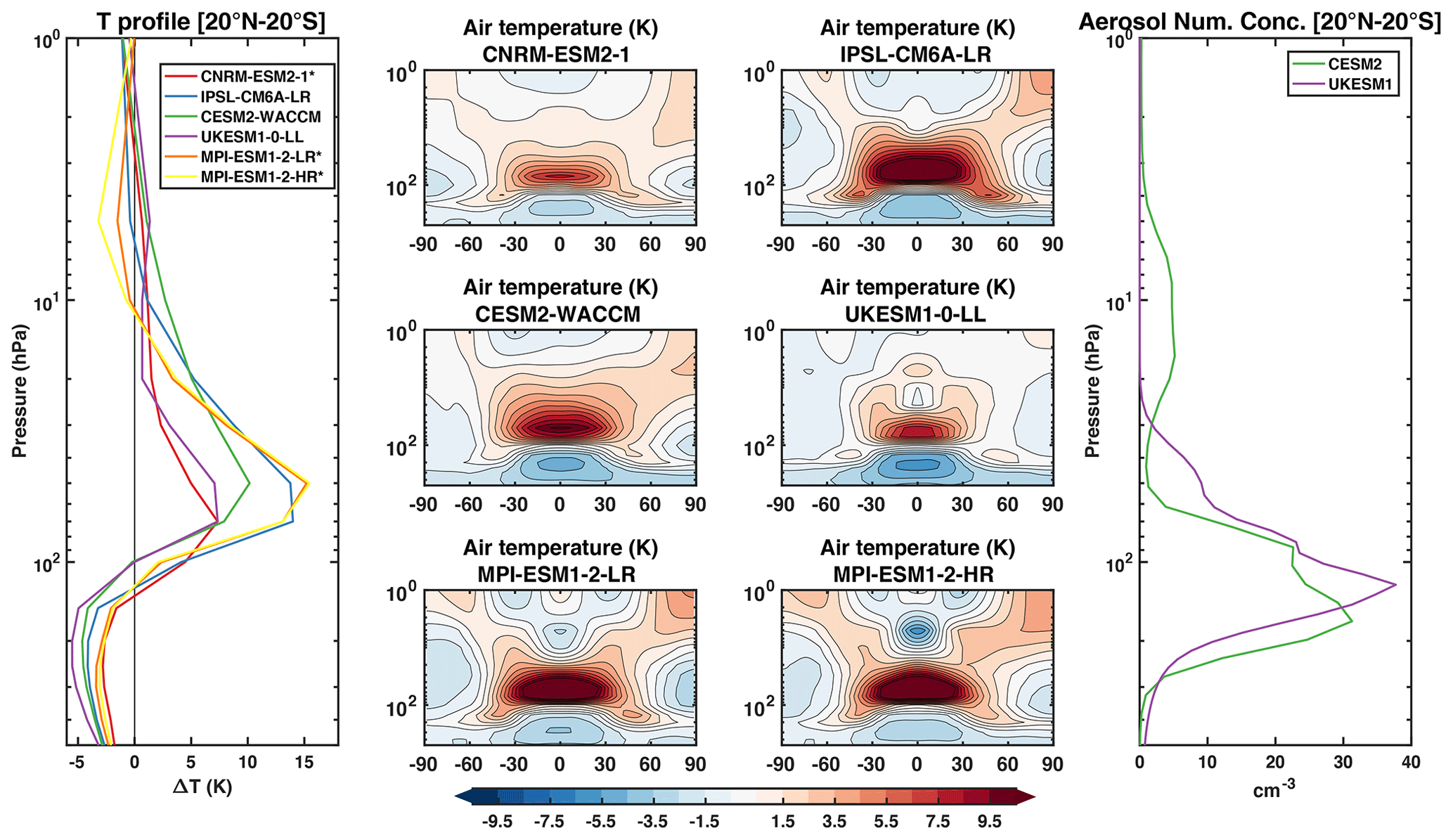
Figure 5Profile of stratospheric temperature changes (G6sulfur minus SSP5-8.5) between 20∘ N and 20∘ S are shown in the left panel. In the central panels, the changes are shown for each participating model. The profiles of aerosol number concentration are shown in the right panel for a select number of models where output was available. All changes are for the years 2081–2100 and evaluated against the same period for the underlying emission scenario SSP5-8.5.
3.3 Surface climate response
When geoengineering the climate, reducing incoming solar radiation (either by simulating stratospheric aerosols or by reducing the solar constant in models) to obtain the same global surface temperature as a scenario with lower GHGs does not assure that regional temperatures follow the same pattern. This has been reported in climate model simulations of various complexity, from 1-D models (Henry and Merlis, 2020) to Earth system model simulations (i.e., Ban-Weiss and Caldeira, 2010; Niemeier et al., 2013; Jones et al., 2018; Visioni et al., 2021). These differences may be reduced if, together with reducing global temperatures, the geoengineering strategy also aims to reduce differences in higher-order temperature gradients (Kravitz et al., 2016; Tilmes et al., 2018a), but they cannot be completely canceled due to various factors. The main factor would be a fundamental difference in the radiative perturbation from CO2 (that warm throughout the atmospheric column) and from the reduction in solar constant (that cool from the bottom-up)(Ban-Weiss and Caldeira, 2010; Henry and Merlis, 2020); then, seasonal and latitudinal differences (Govindasamy et al., 2003; Ban-Weiss and Caldeira, 2010; Visioni et al., 2020b) and surface climate effects (such as precipitation changes) of the stratospheric heating produced by the aerosols (Simpson et al., 2019; Visioni et al., 2021; Jones et al., 2021). Other factors may also be an inability to restore the same state for the ocean circulation. This latter point has been observed, for instance, in CESM1(WACCM) in Fasullo et al. (2018) and in one of the models that performed G6 simulations, CESM2(WACCM), in Tilmes et al. (2020).
All of these differences are compounded with those already present in climate models for regional temperature projections for CO2 increases. On this point, however, MacMartin et al. (2015) argued that reducing surface temperatures through geoengineering has the potential to actually reduce model spread in regional projections. That work, however, considered the G1 experiment, which entails a uniform solar reduction to reduce temperatures under a 4×CO2 increase. Clearly then, most of the differences listed above are not included in such an idealized experiment. This is clear when looking at the multi-model averages of surface temperature differences shown in Fig. 6. The simulated differences with SSP2-4.5 are much larger in G6sulfur compared to G6solar and the inter-model spread is also much larger in G6sulfur. This indicates that there is better agreement between models when the uncertainties related to the stratospheric sulfate are removed. For G6sulfur, there is a general agreement in the inability of sulfate geoengineering to completely cool down the northern high latitudes, partly due to the focus of the geoengineering strategy on reducing global mean temperatures (Kravitz et al., 2019) but also probably due to the presence of stratospheric heating (Jiang et al., 2019), as evident by the absence of high-latitude warming with the same magnitude in the G6solar simulations. The residual warming also present in the G6solar simulations can be partly explained by the differences in the radiative forcing from the CO2 and solar reduction (Ban-Weiss and Caldeira, 2010; Henry and Merlis, 2020; Visioni et al., 2021). Differences in the surface response between models would thus depend on how different models physically reproduce some of the processes mentioned but also on the differences in the stratospheric response reported in the previous section. Different latitudinal and seasonal distributions of the aerosols produce different climate states even in the same model (as shown in CESM1(WACCM) in Kravitz et al., 2019; Visioni et al., 2020b), and the stratospheric heating is also reportedly different, as shown in Fig. 5. Nonetheless, the essential finding from MacMartin et al. (2015) still holds when comparing the multi-model standard error for the geoengineering projections against those for the SSP5-8.5 changes: that especially over land and at high latitudes inter-model differences are always higher than both G6 cases.

Figure 6(a, c, e) Multi-model averages for surface temperature changes averaged over 2081–2100 in different cases: (a) SSP5-8.5, (c) G6sulfur, and (e) G6solar minus the same period for SSP2-4.5. Etched areas (in gray) indicate where less than 66 % of the models (here, four out of six) agree on the sign of the difference in that grid point. Note the different color bar between panel (a) and panels (c)–(e). (b, d, f) Standard error in the multi-model mean for the same reference case on the left. All model results have been re-gridded using a common grid equivalent to that from the model with the lowest horizontal resolution.
We report the surface temperature maps for the last two decades of the experiment for each model in Fig. 7, from which some observations can be made that would not be immediately evident from the multi-model average. For G6sulfur, there is good agreement regarding the residual warming over northern Eurasia across models, with the exception of CESM2. There is less agreement over North America, where some models simulate a cooling in G6sulfur compared to SSP2-4.5 while some simulate a warming. This might be due to differences in the response of the North Atlantic circulation both to increasing GHGs and to geoengineering (Tilmes et al., 2018a, 2020). Comparing this result to that from G6solar, where there is a concurrence of all models in simulating a small warming over the same region, could indicate that the much different response in G6sulfur might on the other hand be due to differences in the distribution of the stratospheric aerosols. UKESM1-0-LL, for instance, where more residual warming is present, shows the lowest AOD over high latitudes (Fig. 4). In the tropics, the Amazon region models seem to differ more in the G6sulfur case and less in the G6solar case; possible causes might be an influence from the different magnitude of AOD in that region, different responses of the vegetation to increasing CO2 concentrations and reduced solar radiation (Simpson et al., 2019) or local changes in atmospheric circulation (Jones et al., 2018).
Overall, the inter-model differences indicate the need for some care when trying to understand the possible surface impacts of sulfate geoengineering by using multi-model ensembles. It might be difficult to correctly separate the differences in surface impacts due to differences in the stratospheric AOD (shown in Fig. 4) given a similar injection and those produced by different response of the surface climate. While comparing results with those from a similar, more uniform experimental design such as G6solar might help, the lack of the potential response produced by the aerosols (Banerjee et al., 2021; Visioni et al., 2021) may suggest the use of a prescribed aerosol distribution for various models (Tilmes et al., 2015) as an intermediate approach. This can also be seen in the comparison between the two versions of MPI (that differ only in their horizontal resolution, which is twice as high in the HR version). They both use the same AOD distribution and have the same magnitude of stratospheric AOD in the whole period. Yet, they show some considerable differences in the surface temperature response to the same aerosol (or even solar) forcing. In particular, the warming observed over North America in the LR version is not as high in the HR version, whereas the warming present in West Antarctica in the HR version is not present in the LR version. This might indicate that the regional temperature response is due to a different deep ocean circulation response (in the West Antarctica case), as also shown in McCusker et al. (2015), and that this might be model dependent (other than being dependent on the particular injection strategy) or due to a different response of the atmospheric circulation (Jones et al., 2018). On the other hand, parts of the response, such as the patches of warming present in the Amazon and in Central Africa, possibly due to a different land response, are shared between the two versions and similarly a large part of the warming over Eurasia. While observing the response of different versions of the same model to the same forcing might point to some of the causes, comparing that to the response of a different model to the same forcing may also highlight which parts of the overall response is model dependent and which are robust across models.
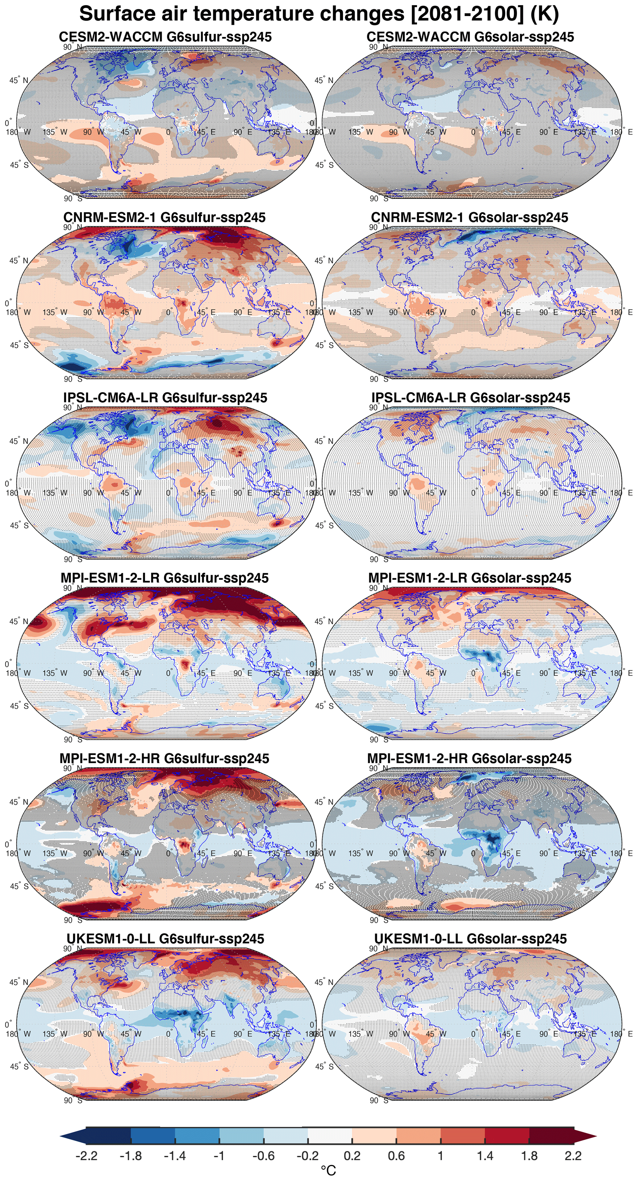
Figure 7Surface temperatures changes in the period 2081–2100 in G6sulfur compared to the same period for SSP2-4.5 in G6sulfur simulations (left panels) and G6solar simulations (right panels) for all participating models. Shaded areas indicate where the difference is not statistically significant, as evaluated using a double-sided t-test with p<0.05 on the ensemble averages for each model and considering all 20 years as independent samples.
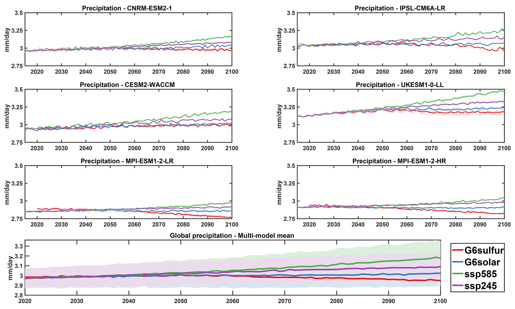
Figure 8Global mean precipitation (mm/day) for the four experiments for each participating model. The multi-models mean is shown at the bottom, with the shading representing 1σ standard deviation of the mean for each experiment.
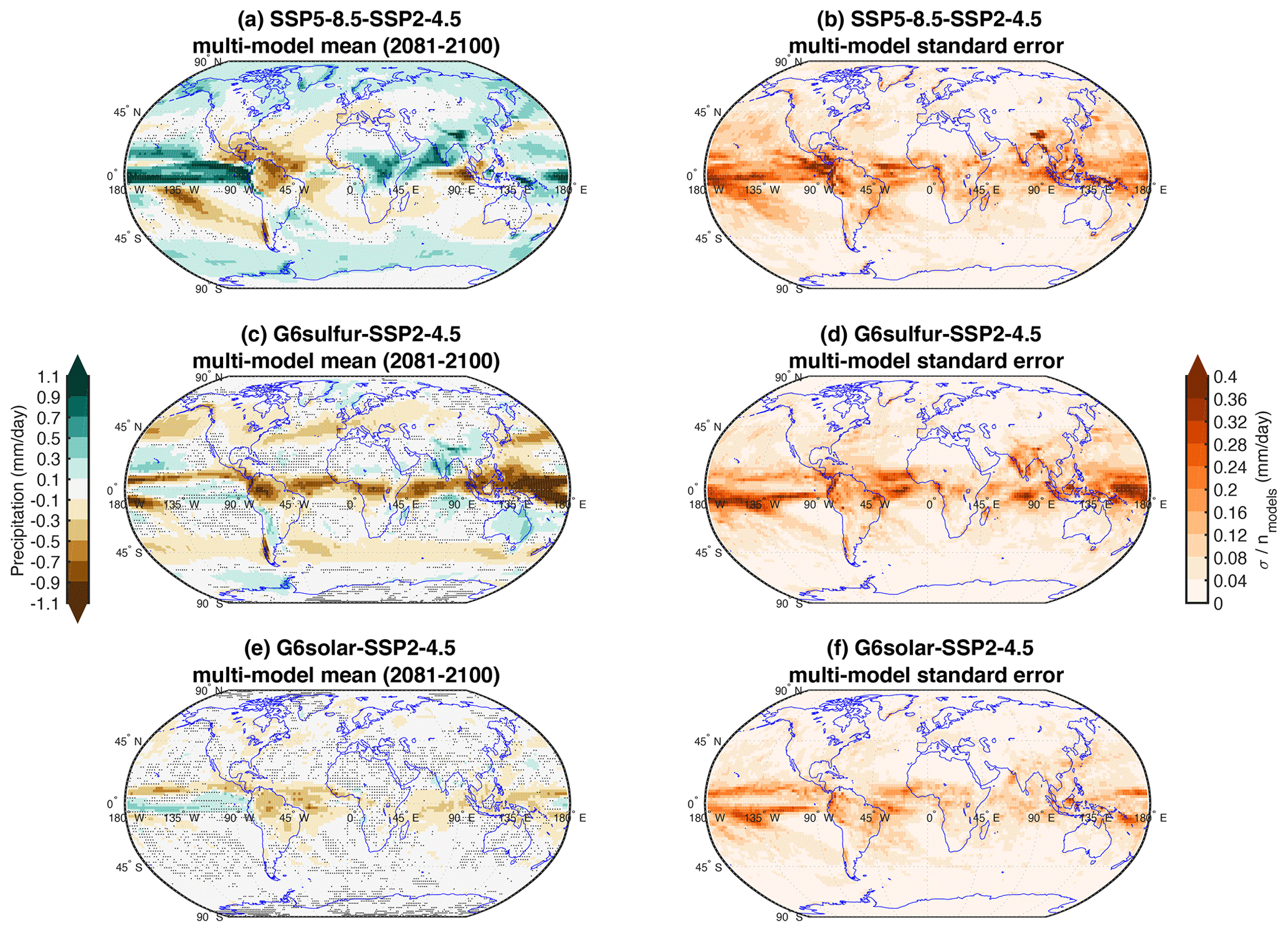
Figure 9(a, c, e) Multi-model averages for precipitation changes averaged over 2081–2100 in different cases: (a) SSP5-8.5, (c) G6sulfur, and (e) G6solar minus the same period for SSP2-4.5. Etched areas (in gray) indicate where less than 66 % of models (here, four out of six) agree on the sign of the difference in that grid point. (b, d, f) Standard error in the multi-model mean for the same reference case on the left. All models results have been re-gridded using a common grid equivalent to that from the model with the lowest horizontal resolution.
Surface temperatures are not the only measure of the possible impacts of either climate change or geoengineering; amongst the many others, hydrological cycle changes are also central to any assessment. Under climate change, due to the surface and tropospheric warming allowing for more moisture to be retained by the air, global precipitation has been consistently projected to increase (Pendergrass and Hartmann, 2014) and a similar behavior is displayed by the models participating in the G6 experiments (Fig. 8). Similarly, it has been widely assessed that trying to restore surface temperature to a previous state by means of modifying the top of the atmosphere radiative balance tends to overcompensate the changes in precipitation, therefore reducing global mean precipitation. Globally, the changes are driven by the perturbation of the surface heat fluxes (Tilmes et al., 2013; Kravitz et al., 2013b; Niemeier et al., 2013) and changes in sea–land temperature contrast. Regionally, however, the modification of the baseline distribution of precipitation can be due to changes in the inter-tropical convergence zone (ITCZ; Russotto and Ackerman, 2018b; Cheng et al., 2019) produced by changes in the inter-hemispheric temperature gradient, general circulation changes produced by stratospheric heating (Simpson et al., 2019) and regional and seasonal changes in heat fluxes and temperature gradients (Jones et al., 2018; Visioni et al., 2020b). In the case of sulfate injections, these changes can be strongly dependent on latitudinal and temporal distribution of the aerosol cloud as well (Kravitz et al., 2019; Visioni et al., 2020b).

Figure 10Precipitation changes (mm/day) in the period 2081–2100 in G6sulfur compared to the same period for SSP2-4.5 in G6sulfur simulations (left panels) and G6solar simulations (right panels) for all participating models. Shaded areas indicate where the difference is not statistically significant, as evaluated using a double-sided t-test with p<0.05 and considering all 20 years as independent samples.
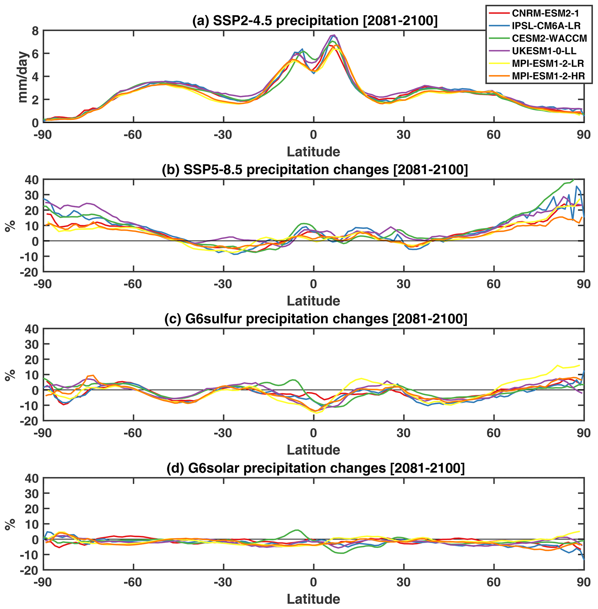
Figure 11(a) Zonal mean precipitation (mm/day) in the period 2081–2100 in SSP2-4.5. (b) Precipitation changes (%) compared to SSP2-4.5 in the same period for SSP5-8.5. (c–d) as in (b), but for G6sulfur and G6solar, respectively.
The response of the various models for the G6 experiments in Fig. 8 consistently shows that the global mean precipitation would be overcompensated (Niemeier et al., 2013). However, models disagree on the magnitude of this overcompensation and in the difference between G6solar and G6sulfur. The fact that under the SSP2-4.5 scenario some warming continues during the 21st century, combined with the precipitation overcompensation by geoengineering, results in some models having no changes in global precipitation compared to the beginning of the century (as already noted in Irvine and Keith, 2020); only G6sulfur in IPSL-CM6A-LR shows a decrease compared to that period by the end of the century. For the purpose of future analyses, the anomalous global precipitation response in the MPI models for G6sulfur has to be noted. It is very likely that the slightly larger response in global mean precipitation at the beginning of the century is due to differences in the initialization process for those simulations rather than in a change produced by the sulfate (which is very close to zero, in 2020) and results before 2050 (for the LR version) or 2040 (for the HR version) should not be considered as representative.
From the perspective of assessing ecosystem impacts, this decoupling of precipitation, temperatures and CO2 should be investigated in depth to understand if and where it would be beneficial or not. It also further stresses the notion that reducing precipitation is not an automatic result of geoengineering but that the outcome is related to which specific cooling targets geoengineering is deployed to achieve (Tilmes et al., 2013; Irvine et al., 2019; Lee et al., 2020). All models agree, to various degrees, that global precipitation changes under G6sulfur are larger than the same changes under G6solar. There might be various reasons for this, such as differences in latent heat due to different ratios of diffuse solar radiation (that increases in the case of the sulfate aerosols; Visioni et al., 2021) resulting in more atmospheric absorption or changes in cloud formation produced by the different vertical atmospheric temperature gradient. Niemeier et al. (2013) suggested that the reason for this might be found in the stratospheric heating produced by the aerosols resulting in more water vapor entering the stratosphere from the warming of the tropopause layer (Tilmes et al., 2018a; Simpson et al., 2019) producing a small positive radiative forcing whose warming effect (Hansen et al., 2005; Visioni et al., 2017a) needs to be counterbalanced by injecting slightly more aerosols.
Lastly, models agree on regional precipitation changes more in G6solar than in G6sulfur (Fig. 9), but all models project most of the significant changes will occur over the tropics (where most of the baseline precipitation is also located), although with some significant local differences between models (Fig. 10). For instance, while CESM2-WACCM shows less precipitation in the tropical Northern Hemisphere and more precipitation in the tropical Southern Hemisphere, UKESM1-0-LL presents a drying in both hemispheres, especially over continents. In some cases, such as at high northern latitudes, all models show a positive change in G6sulfur and a negative change in G6solar. It is again interesting to note the differences in the projected precipitation changes in the two versions of MPI. The HR version shows both further decreases and increases in precipitation in the tropics compared to the LR version, and at high latitudes LR shows much higher changes compared to HR. This shows that even given the same AOD distribution and similar models, some of the observed changes in the case of SAI may differ depending on the simulated response of the circulation to the same forcing, which in the two versions of MPI could be caused by the different horizontal resolution. In this work we have only analyzed the annual response to precipitation, but there are many regions where changes to the seasonal cycle of precipitation may be even more crucial, such as those that experience a monsoon climate and whose cycle might be affected by SAI (see, for instance, Simpson et al., 2019; Visioni et al., 2020b for the Indian subcontinent, and Da-Allada et al., 2020 for western Africa); an in depth analyses of these impacts would also be necessary. Interestingly, unlike for the surface temperatures multi-model standard error (Fig. 6), the standard error for precipitation is very similar and in some cases higher in G6sulfur than in SSP5-8.5.
This indicates that while it is true that reducing surface temperatures would indeed reduce disagreement in future projections between models, this might not hold true for other impacts (of which precipitation might only be an example). For them, due to the influence of changes in surface temperatures, effects driven by CO2 (both radiative and physiological) and possible changes in dynamical perturbations driven by the aerosols, modeling uncertainties might remain higher either with high CO2 or with geoengineering. Some of the drivers of uncertainty may be observed by looking at global and land mean precipitation changes in the last 20 years. For the former, the multi-model mean projects an increase of 2.28 ± 0.80 % compared to SSP2-4.5 in the same period, while it projects a decrease of −3.79 ± 0.76 % for G6sulfur (compared to −2.07 ± 0.40 % for G6solar). For the latter, the SSP5-8.5 increase is 1.53 ± 0.73 %, while for G6sulfur the decrease is −3.96 ± 1.50 %, and −2.35 ± 0.79 % (see Fig. S3 in the Supplement for the results of the single models). For both G6sulfur and SSP5-8.5, the spread of the precipitation response over land is much larger compared to G6solar, and depending on the model there are different responses when comparing the global mean versus the land-mean. As this could be due to a variety of factors, future studies should try to elucidate what is causing these different responses in the various models.
We have shown in this work some preliminary results from the G6sulfur and G6solar modeling experiments proposed in Kravitz et al. (2015) for the Geoengineering Model Intercomparison Project as part of the Climate Model Intercomparison Project Phase 6. These two new experiments aim to reduce global temperatures in the 21st century from those simulated under a high-tier emissions scenario (SSP5-8.5) to those simulated under a medium-tier emissions scenario (SSP2-4.5), either by simulating the artificial injection of stratospheric aerosol precursors in the stratosphere or by reducing the solar constant in the models. In terms of surface climate response, some broad features are shared by all models, such as a reduction in global mean precipitation compared to both SSP scenarios and a residual warming in the northern high latitudes (Henry and Merlis, 2020), which is particularly present in G6sulfur (Simpson et al., 2019; Banerjee et al., 2021). Other locations show more disagreements between models in terms of the surface temperature response. Since there is a larger uniformity in the response between G6solar simulations, where the solar dimming is applied in the same latitudinally uniform way in all models, this suggests that part of the surface response uncertainty in G6sulfur is driven by differences in the latitudinal distribution of the aerosols and not to a different response of the surface climate to the same radiative forcing.
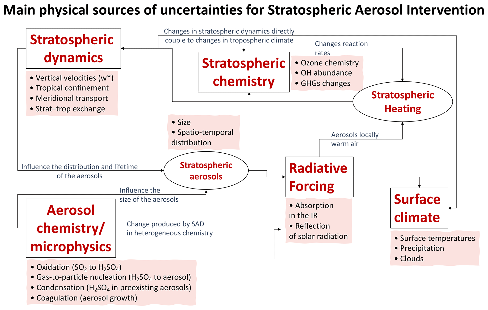
Figure 12Scheme exemplifying the sources of uncertainties in modeling stratospheric aerosols in the context of sulfate geoengineering. Components of the Earth system (and more particularly of the atmosphere, i.e., stratospheric dynamics) are in boxes. In each box, the main processes that would affect (and be affected by) the injection of SO2 in the stratosphere are listed (red shading) and interactions between components are represented by arrows with an explanation in gray. “Stratospheric aerosols” and “Stratospheric heating” are in circles to distinguish them from underlying system components, as they can be considered a single component that is affected and affects multiple things in turn. w residual vertical velocity.
The comparison of the two experiments may help in various ways. When comparing the single-model response to the two different forcings, it helps highlight some of the physical differences between the two interventions (as in Visioni et al., 2021) produced by the stratospheric aerosols' physical and chemical effects. Analyzing the inter-model spread also highlights the degree to which uncertainty in surface climate response to stratospheric aerosols is driven by uncertainties in the stratospheric processes versus uncertainties in how the climate response to a specified forcing such as reduced insolation and may point to a path to successfully identify and, eventually, reduce some of them. We have shown that large inter-model variability remains in the distribution of the aerosol after injections of SO2 in the tropical stratosphere as well as in the temperature response of the stratosphere. As we discussed in Sect. 3.2, the resulting latitudinal distribution of the aerosols given similar injection locations can be due to multiple factors, such as the stratospheric dynamics differences regulating the large-scale transport of the aerosols and the microphysical differences regulating the oxidation of SO2 and the subsequent growth of the aerosols. The interaction between the stratospheric aerosols and the rest of the system further complicates the identification of a single mechanism by which aerosol distributions might differ. There may be uncertainties related to the simulated radiative interaction (for instance, the rate of absorption of IR radiation by the aerosols) and stratospheric chemistry (i.e., changes in ozone chemistry, which in turn affects local radiative transfer) that produce different localized heating of air and thus affect differently both the surface climate and stratospheric dynamics (which in turn may affect the aerosol distribution; Niemeier and Schmidt, 2017; Kleinschmitt et al., 2018). All these uncertainties in stratospheric dynamics (summarized in Fig. 12) can thus indirectly affect surface climate in simulations of geoengineering with stratospheric aerosols by means of a different reflection of sunlight depending on the resulting distribution of the aerosols. This type of uncertainty is thus separated from those directly connected to a stratospheric influence on various aspects of the surface climate: local surface temperatures (Jiang et al., 2019), precipitation (Simpson et al., 2019) or cloud cover changes (Visioni et al., 2018a).
Simulations such as those we analyzed here can give useful information on the current range of uncertainty over many projected impacts of geoengineering. In particular, the successful coupling of the new Earth system models used in CMIP6 with land, ocean and cryosphere components can help with the exploration of various impacts, for instance, on ecosystems (Zarnetske et al., 2021) or ice sheets melting (Fettweis et al., 2020), which are crucial to properly inform policymakers and interested parties, and the inter-model spread can help in communicating the uncertainties tied to those projections. As we outlined above, however, these simulations may not be as useful in helping reduce most of these uncertainties. It is therefore important not to rely only on these simulations going forward but to devise new experiments that might improve the accuracy with which we model the relevant interactions in the atmosphere. To do so, there may be multiple venues. One way could be using different physical-based approaches to modeling that do not involve 3-D climate modeling and that might shed light on the single processes (for instance, Dai et al., 2018; Lutsko et al., 2020; Seeley et al., 2021 or plume modeling), such as lab experiments trying to replicate the conditions of the stratosphere (Dai et al., 2020). Another way could be using global climate models but trying to constrain some of the various processes in order to reduce uncertainty. This could be done, for instance, by prescribing the same stratospheric aerosol distribution in different models (as suggested in Tilmes et al., 2015), as some models do in this work, by modifying some parameters in the model simulation while keeping everything else fixed to constrain a source of uncertainty (as proposed for volcanic eruption by Timmreck et al. (2018) in the Pinatubo Emulation in Multiple models (PoEMs) experiment), or by continuing to simulate a constant solar dimming in place of the more complex aerosols (see, for instance, Irvine et al., 2019) to understand portions of the global surface response. All of these methods combined (and more) may be able to increase our confidence when projecting the impacts of sulfate geoengineering as a short-term addition to mitigation (but not as its replacement; MacMartin et al., 2018; de Coninck et al., 2018) in order to limit the harmful impacts of climate change.
When considering the possible impacts of SAI using GeoMIP simulations, it should also be considered that the injection strategy simulated in the G6 experiments is only one of the possible ways in which SAI could be deployed and, for various reasons, it may not even be the most ideal. Kravitz et al. (2019) showed that a strategy that makes use of different locations of injection outside the Equator (MacMartin et al., 2017) in order to manage not just global mean temperatures but also inter-hemispheric and Equator-to-pole temperature gradients would further reduce harmful impacts by better restoring sea-ice and maintain the ITCZ location. Further, injecting all days of the year might also not be the most ideal choice (Visioni et al., 2019) and some of the resulting climatic effects might depend on the seasonal distribution of the aerosol cloud (Visioni et al., 2020b). So, while the coordinated experiment described in this work might be good as a starting point, it should not be considered as the only way in which SAI might be deployed. This is also valid in terms of the underlying emission scenario used, as a future where emissions continue unabated (which is the case for SSP5-8.5, the scenario used for the G6 experiments) is absolutely not the ideal one in which an eventual SAI deployment should be imagined, even if it might mitigate the short-term effects of the GHG-induced warming. A scenario where emissions are cut, but not fast enough, and global temperature thresholds set by international agreements may be temporarily exceeded could be one where a limited deployment of SAI might be considered as a short-term mitigation strategy with more limited consequences on the environment (Tilmes et al., 2020).
All data used in this work are available from the Earth System Grid (https://esgf-node.llnl.gov/search/cmip6/, WCRP, 2021).
The supplement related to this article is available online at: https://doi.org/10.5194/acp-21-10039-2021-supplement.
DV performed the analyses and wrote the manuscript. DGM and BK helped with the analyses and advised DV throughout the writing process. OB, AJ, LT, MM, MJM, PN, UN, RS and ST performed the simulations and offered valuable comments on the manuscript.
The authors declare that they have no conflict of interest.
Publisher's note: Copernicus Publications remains neutral with regard to jurisdictional claims in published maps and institutional affiliations.
This article is part of the special issue “Resolving uncertainties in solar geoengineering through multi-model and large-ensemble simulations (ACP/ESD inter-journal SI)”. It is not associated with a conference.
Support for DGM was provided by the National Science Foundation through agreement CBET-1818759. Support for Daniele Visioni was provided by the Atkinson Center for a Sustainable Future at Cornell University. Support for Ben Kravitz was provided in part by the National Sciences Foundation through agreement CBET-1931641, the Indiana University Environmental Resilience Institute, and the Prepared for Environmental Change Grand Challenge initiative. The Pacific Northwest National Laboratory is operated for the U.S. Department of Energy by Battelle Memorial Institute under contract DE-AC05-76RL01830. This work benefited from the French state aid managed by the ANR under the “Investissements d'avenir” programme with reference ANR-11-IDEX-0004-17-EURE-0006. Andy Jones was supported by the Met Office Hadley Centre Climate Programme funded by the UK Government Department for Business, Energy and Industrial Strategy (BEIS) and the UK Government Department for Environment, Food and Rural Affairs (Defra). Ulrike Niemeier was supported by the Deutsche Forschungsgemeinschaft Research Unit VollImpact (FOR2820). Michou Martine, Pierre Nabat, Olivier Boucher and Roland Séférian acknowledge support from the European Union's Horizon 2020 research and innovation programme under grant agreement No 820829 (CONSTRAIN) and thank the support of the team in charge of the CNRM-CM climate model. MPI-ESM were performed on the Deutsches Klima Rechenzentrum (DKRZ) computer. The CESM project is supported primarily by the National Science Foundation. The IPSL-CM6 experiments were performed using the HPC resources of TGCC under the allocations 2019-A0060107732 and 2020-A0080107732 (project gencmip6) provided by GENCI (Grand Equipement National de Calcul Intensif). Supercomputing time for CNRM-ESM-2 was provided by the Météo-France/DSIsupercomputing center.
Douglas MacMartin and Ben Kravitz have been supported by the National Science Foundation (USA) (grant nos. CBET-1818759 and CBET-1931641). Ulrike Niemeier has been supported by the Deutsche Forschungsgemeinschaft Research Unit VolImpact (grant no. FOR2820). Michou Martine, Pierre Nabat, Olivier Boucher and Roland Séfŕian have been supported by the European Union's 90 Horizon 2020 research and innovation program (CONSTRAIN (grant no. 820829)).
This paper was edited by Anja Schmidt and reviewed by Peter Irvine and two anonymous referees.
Aquila, V., Garfinkel, C., Newman, P., Oman, L., and Waugh, D.: Modifications of the quasi-biennial oscillation by a geoengineering perturbation of the stratospheric aerosol layer, Geophys. Res. Lett., 41, 1738–1744, 2014. a, b
Arora, V. K., Katavouta, A., Williams, R. G., Jones, C. D., Brovkin, V., Friedlingstein, P., Schwinger, J., Bopp, L., Boucher, O., Cadule, P., Chamberlain, M. A., Christian, J. R., Delire, C., Fisher, R. A., Hajima, T., Ilyina, T., Joetzjer, E., Kawamiya, M., Koven, C. D., Krasting, J. P., Law, R. M., Lawrence, D. M., Lenton, A., Lindsay, K., Pongratz, J., Raddatz, T., Séférian, R., Tachiiri, K., Tjiputra, J. F., Wiltshire, A., Wu, T., and Ziehn, T.: Carbon–concentration and carbon–climate feedbacks in CMIP6 models and their comparison to CMIP5 models, Biogeosciences, 17, 4173–4222, https://doi.org/10.5194/bg-17-4173-2020, 2020. a
Aswathy, V. N., Boucher, O., Quaas, M., Niemeier, U., Muri, H., Mülmenstädt, J., and Quaas, J.: Climate extremes in multi-model simulations of stratospheric aerosol and marine cloud brightening climate engineering, Atmos. Chem. Phys., 15, 9593–9610, https://doi.org/10.5194/acp-15-9593-2015, 2015. a
Ban-Weiss, G. A. and Caldeira, K.: Geoengineering as an optimization problem, Environ. Res. Lett., 5, https://doi.org/10.1088/1748-9326/5/3/034009, 2010. a, b, c, d
Banerjee, A., Butler, A. H., Polvani, L. M., Robock, A., Simpson, I. R., and Sun, L.: Robust winter warming over Eurasia under stratospheric sulfate geoengineering – the role of stratospheric dynamics, Atmos. Chem. Phys., 21, 6985–6997, https://doi.org/10.5194/acp-21-6985-2021, 2021. a, b, c
Boucher, O., Kleinschmitt, C., and Myhre, G.: Quasi-Additivity of the Radiative Effects of Marine Cloud Brightening and Stratospheric Sulfate Aerosol Injection, Geophys. Res. Lett., 44, 11158–11165, https://doi.org/10.1002/2017GL074647, 2017. a
Boucher, O., Denvil, S., Levavasseur, G., Cozic, A., Caubel, A., Foujols, M.-A., Meurdesoif, Y., Cadule, P., Devilliers, M., Ghattas, J., Lebas, N., Lurton, T., Mellul, L., Musat, I., Mignot, J., and Cheruy, F.: IPSL IPSL-CM6A-LR model output prepared for CMIP6 CMIP historical, Earth System Grid Federation, https://doi.org/10.22033/ESGF/CMIP6.5195, 2018. a
Boucher, O., Servonnat, J., Albright, A. L., Aumont, O., Balkanski, Y., Bastrikov, V., Bekki, S., Bonnet, R., Bony, S., Bopp, L., Braconnot, P., Brockmann, P., Cadule, P., Caubel, A., Cheruy, F., Codron, F., Cozic, A., Cugnet, D., D'Andrea, F., Davini, P., de Lavergne, C., Denvil, S., Deshayes, J., Devilliers, M., Ducharne, A., Dufresne, J.-L., Dupont, E., Éthé, C., Fairhead, L., Falletti, L., Flavoni, S., Foujols, M.-A., Gardoll, S., Gastineau, G., Ghattas, J., Grandpeix, J.-Y., Guenet, B., Guez, Lionel, E., Guilyardi, E., Guimberteau, M., Hauglustaine, D., Hourdin, F., Idelkadi, A., Joussaume, S., Kageyama, M., Khodri, M., Krinner, G., Lebas, N., Levavasseur, G., Lévy, C., Li, L., Lott, F., Lurton, T., Luyssaert, S., Madec, G., Madeleine, J.-B., Maignan, F., Marchand, M., Marti, O., Mellul, L., Meurdesoif, Y., Mignot, J., Musat, I., Ottlé, C., Peylin, P., Planton, Y., Polcher, J., Rio, C., Rochetin, N., Rousset, C., Sepulchre, P., Sima, A., Swingedouw, D., Thiéblemont, R., Traore, A. K., Vancoppenolle, M., Vial, J., Vialard, J., Viovy, N., and Vuichard, N.: Presentation and Evaluation of the IPSL-CM6A-LR Climate Model, J. Adv. Model. Earth Sy., 12, e2019MS002010, https://doi.org/10.1029/2019MS002010, 2020. a
Budyko, M. I.: Climatic Changes, Vol. 10, chap. 7: The Climate of the Future, American Geophysical Union, https://doi.org/10.1029/SP010, 1977. a
Canty, T., Mascioli, N. R., Smarte, M. D., and Salawitch, R. J.: An empirical model of global climate – Part 1: A critical evaluation of volcanic cooling, Atmos. Chem. Phys., 13, 3997–4031, https://doi.org/10.5194/acp-13-3997-2013, 2013. a
Cheng, W., MacMartin, D. G., Dagon, K., Kravitz, B., Tilmes, S., Richter, J. H., Mills, M. J., and Simpson, I. R.: Soil Moisture and Other Hydrological Changes in a Stratospheric Aerosol Geoengineering Large Ensemble, J. Geophys. Res.-Atmos., 124, 12773–12793, https://doi.org/10.1029/2018JD030237, 2019. a
Clyne, M., Lamarque, J.-F., Mills, M. J., Khodri, M., Ball, W., Bekki, S., Dhomse, S. S., Lebas, N., Mann, G., Marshall, L., Niemeier, U., Poulain, V., Robock, A., Rozanov, E., Schmidt, A., Stenke, A., Sukhodolov, T., Timmreck, C., Toohey, M., Tummon, F., Zanchettin, D., Zhu, Y., and Toon, O. B.: Model physics and chemistry causing intermodel disagreement within the VolMIP-Tambora Interactive Stratospheric Aerosol ensemble, Atmos. Chem. Phys., 21, 3317–3343, https://doi.org/10.5194/acp-21-3317-2021, 2021. a, b
Crutzen, P. J.: Albedo Enhancement by Stratospheric Sulfur Injections: A Contribution to Resolve a Policy Dilemma?, Climatic Change, 77, 211–220, https://doi.org/10.1007/s10584-006-9101-y, 2006. a
Da-Allada, C. Y., Baloïtcha, E., Alamou, E. A., Awo, F. M., Bonou, F., Pomalegni, Y., Biao, E. I., Obada, E., Zandagba, J. E., Tilmes, S., and Irvine, P. J.: Changes in West African Summer Monsoon Precipitation Under Stratospheric Aerosol Geoengineering, Earth's Future, 8, e2020EF001595, https://doi.org/10.1029/2020EF001595, 2020. a
Dai, Z., Weisenstein, D. K., and Keith, D. W.: Tailoring Meridional and Seasonal Radiative Forcing by Sulfate Aerosol Solar Geoengineering, Geophys. Res. Lett., 45, 1030–1039, https://doi.org/10.1002/2017GL076472, 2018. a
Dai, Z., Weisenstein, D. K., Keutsch, F. N., and Keith, D. W.: Experimental reaction rates constrain estimates of ozone response to calcium carbonate geoengineering, Commun. Earth Environ., 1, 63, https://doi.org/10.1038/s43247-020-00058-7, 2020. a
Danabasoglu, G.: NCAR CESM2-WACCM model output prepared for CMIP6 CMIP, Earth System Grid Federation, https://doi.org/10.22033/ESGF/CMIP6.10024, 2019. a
Danabasoglu, G., Lamarque, J.-F., Bacmeister, J., Bailey, D. A., DuVivier, A. K., Edwards, J., Emmons, L. K., Fasullo, J., Garcia, R., Gettelman, A., Hannay, C., Holland, M. M., Large, W. G., Lauritzen, P. H., Lawrence, D. M., Lenaerts, J. T. M., Lindsay, K., Lipscomb, W. H., Mills, M. J., Neale, R., Oleson, K. W., Otto-Bliesner, B., Phillips, A. S., Sacks, W., Tilmes, S., van Kampenhout, L., Vertenstein, M., Bertini, A., Dennis, J., Deser, C., Fischer, C., Fox-Kemper, B., Kay, J. E., Kinnison, D., Kushner, P. J., Larson, V. E., Long, M. C., Mickelson, S., Moore, J. K., Nienhouse, E., Polvani, L., Rasch, P. J., and Strand, W. G.: The Community Earth System Model Version 2 (CESM2), J. Adv. Model. Earth Sy., 12, e2019MS001916, https://doi.org/10.1029/2019MS001916, 2020. a
de Coninck, H., Revi, A., Babiker, M., Bertoldi, P., Buckeridge, M., Cartwright, A., Dong, W., Ford, J., Fuss, S., Hourcade, J.-C., Ley, D., Mechler, R., Newman, P., Revokatova, A., Schultz, S., Steg, L., and Sugiyama, T.: Chapter 4: Strengthening and Implementing the Global Response, in: Global warming of 1.5∘C. An IPCC Special Report on the impacts of global warming of 1.5∘C above pre-industrial levels and related global greenhouse gas emission pathways, in the context of strengthening the global response to the threat of climate change, sustainable development, and efforts to eradicate poverty, edited by: IPCC, IPCC, available at: https://www.ipcc.ch/sr15/chapter/chapter-4/ (last access: 28 June 2021), 2018. a
Dhomse, S. S., Mann, G. W., Antuña Marrero, J. C., Shallcross, S. E., Chipperfield, M. P., Carslaw, K. S., Marshall, L., Abraham, N. L., and Johnson, C. E.: Evaluating the simulated radiative forcings, aerosol properties, and stratospheric warmings from the 1963 Mt Agung, 1982 El Chichón, and 1991 Mt Pinatubo volcanic aerosol clouds, Atmos. Chem. Phys., 20, 13627–13654, https://doi.org/10.5194/acp-20-13627-2020, 2020. a, b
Duan, L., Cao, L., Bala, G., and Caldeira, K.: Climate Response to Pulse Versus Sustained Stratospheric Aerosol Forcing, Geophys. Res. Lett., 46, 8976–8984, https://doi.org/10.1029/2019GL083701, 2019. a
Fasullo, J. T., Simpson, I. R., Kravitz, B., Tilmes, S., Richter, J. H., MacMartin, D. G., and Mills, M. J.: Persistent polar ocean warming in a strategically geoengineered climate, Nat. Geosci., 11, 910–914, https://doi.org/10.1038/s41561-018-0249-7, 2018. a
Fettweis, X., Hofer, S., Séférian, R., Amory, C., Delhasse, A., Doutreloup, S., Kittel, C., Lang, C., Van Bever, J., Veillon, F., and Irvine, P.: Brief Communication: “Reduction of the future Greenland ice sheet surface melt with the help of solar geoengineering”, The Cryosphere Discuss. [preprint], https://doi.org/10.5194/tc-2020-347, in review, 2020. a
Franke, H., Niemeier, U., and Visioni, D.: Differences in the quasi-biennial oscillation response to stratospheric aerosol modification depending on injection strategy and species, Atmos. Chem. Phys., 21, 8615–8635, https://doi.org/10.5194/acp-21-8615-2021, 2021. a, b, c
Gettelman, A., Hannay, C., Bacmeister, J. T., Neale, R. B., Pendergrass, A. G., Danabasoglu, G., Lamarque, J.-F., Fasullo, J. T., Bailey, D. A., Lawrence, D. M., and Mills, M. J.: High Climate Sensitivity in the Community Earth System Model Version 2 (CESM2), Geophys. Res. Lett., 46, 8329–8337, https://doi.org/10.1029/2019GL083978, 2019. a, b
Glienke, S., Irvine, P. J., and Lawrence, M. G.: The impact of geoengineering on vegetation in experiment G1 of the GeoMIP, J. Geophys. Res.-Atmos., 120, 10196–10213, https://doi.org/10.1002/2015JD024202, 2015. a
Govindasamy, B., Caldeira, K., and Duffy, P.: Geoengineering Earth's radiation balance to mitigate climate change from a quadrupling of CO2, Global Planet. Change, 37, 157–168, https://doi.org/10.1016/S0921-8181(02)00195-9, 2003. a
Hansen, J., Sato, M., Ruedy, R., Nazarenko, L., Lacis, A., Schmidt, G. A., Russell, G., Aleinov, I., Bauer, M., Bauer, S., Bell, N., Cairns, B., Canuto, V., Chandler, M., Cheng, Y., Del Genio, A., Faluvegi, G., Fleming, E., Friend, A., Hall, T., Jackman, C., Kelley, M., Kiang, N., Koch, D., Lean, J., Lerner, J., Lo, K., Menon, S., Miller, R., Minnis, P., Novakov, T., Oinas, V., Perlwitz, J., Perlwitz, J., Rind, D., Romanou, A., Shindell, D., Stone, P., Sun, S., Tausnev, N., Thresher, D., Wielicki, B., Wong, T., Yao, M., and Zhang, S.: Efficacy of climate forcings, J. Geophys. Res.-Atmos, 110, https://doi.org/10.1029/2005JD005776, 2005. a, b
Henry, M. and Merlis, T. M.: Forcing Dependence of Atmospheric Lapse Rate Changes Dominates Residual Polar Warming in Solar Radiation Management Climate Scenarios, Geophys. Res. Lett., 47, e2020GL087929, https://doi.org/10.1029/2020GL087929, 2020. a, b, c, d
Irvine, P., Emanuel, K., He, J., Horowitz, L. W., Vecchi, G., and Keith, D.: Halving warming with idealized solar geoengineering moderates key climate hazards, Nat. Clim. Change, 9, 295–299, https://doi.org/10.1038/s41558-019-0398-8, 2019. a, b
Irvine, P. J. and Keith, D. W.: Halving warming with stratospheric aerosol geoengineering moderates policy-relevant climate hazards, Environ. Res. Lett., 15, 044011, https://doi.org/10.1088/1748-9326/ab76de, 2020. a
Ji, D., Fang, S., Curry, C. L., Kashimura, H., Watanabe, S., Cole, J. N. S., Lenton, A., Muri, H., Kravitz, B., and Moore, J. C.: Extreme temperature and precipitation response to solar dimming and stratospheric aerosol geoengineering, Atmos. Chem. Phys., 18, 10133–10156, https://doi.org/10.5194/acp-18-10133-2018, 2018. a
Jiang, J., Cao, L., MacMartin, D. G., Simpson, I. R., Kravitz, B., Cheng, W., Visioni, D., Tilmes, S., Richter, J. H., and Mills, M. J.: Stratospheric Sulfate Aerosol Geoengineering Could Alter the High-Latitude Seasonal Cycle, Geophys. Res. Lett., 46, 14153–14163, https://doi.org/10.1029/2019GL085758, 2019. a, b, c, d
Jones, A., Haywood, J. M., Jones, A. C., Tilmes, S., Kravitz, B., and Robock, A.: North Atlantic Oscillation response in GeoMIP experiments G6solar and G6sulfur: why detailed modelling is needed for understanding regional implications of solar radiation management, Atmos. Chem. Phys., 21, 1287–1304, https://doi.org/10.5194/acp-21-1287-2021, 2021. a
Jones, A. C., Hawcroft, M. K., Haywood, J. M., Jones, A., Guo, X., and Moore, J. C.: Regional Climate Impacts of Stabilizing Global Warming at 1.5 K Using Solar Geoengineering, Earth's Future, 6, 230–251, https://doi.org/10.1002/2017EF000720, 2018. a, b, c, d
Jungclaus, J., Bittner, M., Wieners, K.-H., Wachsmann, F., Schupfner, M., Legutke, S., Giorgetta, M., Reick, C., Gayler, V., Haak, H., de Vrese, P., Raddatz, T., Esch, M., Mauritsen, T., von Storch, J.-S., Behrens, J., Brovkin, V., Claussen, M., Crueger, T., Fast, I., Fiedler, S., Hagemann, S., Hohenegger, C., Jahns, T., Kloster, S., Kinne, S., Lasslop, G., Kornblueh, L., Marotzke, J., Matei, D., Meraner, K., Mikolajewicz, U., Modali, K., Müller, W., Nabel, J., Notz, D., Peters, K., Pincus, R., Pohlmann, H., Pongratz, J., Rast, S., Schmidt, H., Schnur, R., Schulzweida, U., Six, K., Stevens, B., Voigt, A., and Roeckner, E.: MPI-M MPI-ESM1.2-HR model output prepared for CMIP6 CMIP historical, Earth System Grid Federation, https://doi.org/10.22033/ESGF/CMIP6.6594, 2019. a
Kashimura, H., Abe, M., Watanabe, S., Sekiya, T., Ji, D., Moore, J. C., Cole, J. N. S., and Kravitz, B.: Shortwave radiative forcing, rapid adjustment, and feedback to the surface by sulfate geoengineering: analysis of the Geoengineering Model Intercomparison Project G4 scenario, Atmos. Chem. Phys., 17, 3339–3356, https://doi.org/10.5194/acp-17-3339-2017, 2017. a
Kleinschmitt, C., Boucher, O., and Platt, U.: Sensitivity of the radiative forcing by stratospheric sulfur geoengineering to the amount and strategy of the SO2injection studied with the LMDZ-S3A model, Atmos. Chem. Phys., 18, 2769–2786, https://doi.org/10.5194/acp-18-2769-2018, 2018. a
Kravitz, B. and MacMartin, D. G.: Uncertainty and the basis for confidence in solar geoengineering research, Nat. Rev. Earth Environ., 1, 64–75, https://doi.org/10.1038/s43017-019-0004-7, 2020. a
Kravitz, B., Robock, A., Boucher, O., Schmidt, H., Taylor, K. E., Stenchikov, G., and Schulz, M.: The Geoengineering Model Intercomparison Project (GeoMIP), Atmos. Sci. Lett., 12, 162–167, https://doi.org/10.1002/asl.316, 2011. a
Kravitz, B., Caldeira, K., Boucher, O., Robock, A., Rasch, P. J., Alterskjær, K., Karam, D. B., Cole, J. N. S., Curry, C. L., Haywood, J. M., Irvine, P. J., Ji, D., Jones, A., Kristjánsson, J. E., Lunt, D. J., Moore, J. C., Niemeier, U., Schmidt, H., Schulz, M., Singh, B., Tilmes, S., Watanabe, S., Yang, S., and Yoon, J.-H.: Climate model response from the Geoengineering Model Intercomparison Project (GeoMIP), J. Geophys. Res.-Atmos., 118, 8320–8332, https://doi.org/10.1002/jgrd.50646, 2013a. a
Kravitz, B., Rasch, P. J., Forster, P. M., Andrews, T., Cole, J. N., Irvine, P. J., Ji, D., Kristjánsson, J. E., Moore, J. C., Muri, H., Niemeier, U., Robock, A., Singh, B., Tilmes, S., Watanabe, S., and Yoon, J. H.: An energetic perspective on hydrological cycle changes in the Geoengineering Model Intercomparison Project, J. Geophys. Res.-Atmos., 118, 13087–13102, https://doi.org/10.1002/2013JD020502, 2013b. a, b, c, d
Kravitz, B., Robock, A., Tilmes, S., Boucher, O., English, J. M., Irvine, P. J., Jones, A., Lawrence, M. G., MacCracken, M., Muri, H., Moore, J. C., Niemeier, U., Phipps, S. J., Sillmann, J., Storelvmo, T., Wang, H., and Watanabe, S.: The Geoengineering Model Intercomparison Project Phase 6 (GeoMIP6): simulation design and preliminary results, Geosci. Model Dev., 8, 3379–3392, https://doi.org/10.5194/gmd-8-3379-2015, 2015. a, b, c
Kravitz, B., MacMartin, D. G., Wang, H., and Rasch, P. J.: Geoengineering as a design problem, Earth Syst. Dynam., 7, 469–497, https://doi.org/10.5194/esd-7-469-2016, 2016. a
Kravitz, B., Lamarque, J.-F., Tribbia, J. J., Tilmes, S., Vitt, F., Richter, J. H., MacMartin, D. G., and Mills, M. J.: First Simulations of Designing Stratospheric Sulfate Aerosol Geoengineering to Meet Multiple Simultaneous Climate Objectives, J. Geophys. Res.-Atmos., 122, 12616–12634, https://doi.org/10.1002/2017jd026874, 2017. a
Kravitz, B., MacMartin, D. G., Tilmes, S., Richter, J. H., Mills, M. J., Cheng, W., Dagon, K., Glanville, A. S., Lamarque, J.-F., Simpson, I. R., Tribbia, J., and Vitt, F.: Comparing Surface and Stratospheric Impacts of Geoengineering With Different SO2 Injection Strategies, J. Geophys. Res.-Atmos., 124, 7900–7918, https://doi.org/10.1029/2019JD030329, 2019. a, b, c, d, e, f
Kravitz, B., MacMartin, D. G., Visioni, D., Boucher, O., Cole, J. N. S., Haywood, J., Jones, A., Lurton, T., Nabat, P., Niemeier, U., Robock, A., Séférian, R., and Tilmes, S.: Comparing different generations of idealized solar geoengineering simulations in the Geoengineering Model Intercomparison Project (GeoMIP), Atmos. Chem. Phys., 21, 4231–4247, https://doi.org/10.5194/acp-21-4231-2021, 2021. a, b, c, d
Laakso, A., Snyder, P. K., Liess, S., Partanen, A.-I., and Millet, D. B.: Differing precipitation response between solar radiation management and carbon dioxide removal due to fast and slow components, Earth Syst. Dynam., 11, 415–434, https://doi.org/10.5194/esd-11-415-2020, 2020. a
Lee, W., MacMartin, D., Visioni, D., and Kravitz, B.: Expanding the design space of stratospheric aerosol geoengineering to include precipitation-based objectives and explore trade-offs, Earth Syst. Dynam., 11, 1051–1072, https://doi.org/10.5194/esd-11-1051-2020, 2020. a
Lurton, T., Balkanski, Y., Bastrikov, V., Bekki, S., Bopp, L., Braconnot, P., Brockmann, P., Cadule, P., Contoux, C., Cozic, A., Cugnet, D., Dufresne, J.-L., Éthé, C., Foujols, M.-A., Ghattas, J., Hauglustaine, D., Hu, R.-M., Kageyama, M., Khodri, M., Lebas, N., Levavasseur, G., Marchand, M., Ottlé, C., Peylin, P., Sima, A., Szopa, S., Thiéblemont, R., Vuichard, N., and Boucher, O.: Implementation of the CMIP6 Forcing Data in the IPSL-CM6A-LR Model, J. Adv. Model. Earth Sy., 12, e2019MS001940, https://doi.org/10.1029/2019MS001940, 2020. a
Lutsko, N. J., Seeley, J. T., and Keith, D. W.: Estimating Impacts and Trade-offs in Solar Geoengineering Scenarios With a Moist Energy Balance Model, Geophys. Res. Lett., 47, e2020GL087290, https://doi.org/10.1029/2020GL087290, 2020. a
MacMartin, D. G., Kravitz, B., and Rasch, P. J.: On solar geoengineering and climate uncertainty, Geophys. Res. Lett., 42, 7156–7161, https://doi.org/10.1002/2015GL065391, 2015. a, b
MacMartin, D. G., Kravitz, B., Mills, M. J., Tribbia, J. J., Tilmes, S., Richter, J. H., Vitt, F., and Lamarque, J.-F.: The Climate Response to Stratospheric Aerosol Geoengineering Can Be Tailored Using Multiple Injection Locations, J. Geophys. Res.-Atmos., 122, 12574–12590, https://doi.org/10.1002/2017jd026868, 2017. a, b
MacMartin, D. G., Ricke, K. L., and Keith, D. W.: Solar geoengineering as part of an overall strategy for meeting the 1.5∘C Paris target, Philos. T. R. Soc. A, 376, 20160454, https://doi.org/10.1098/rsta.2016.0454, 2018. a
Marshall, L., Schmidt, A., Toohey, M., Carslaw, K. S., Mann, G. W., Sigl, M., Khodri, M., Timmreck, C., Zanchettin, D., Ball, W. T., Bekki, S., Brooke, J. S. A., Dhomse, S., Johnson, C., Lamarque, J.-F., LeGrande, A. N., Mills, M. J., Niemeier, U., Pope, J. O., Poulain, V., Robock, A., Rozanov, E., Stenke, A., Sukhodolov, T., Tilmes, S., Tsigaridis, K., and Tummon, F.: Multi-model comparison of the volcanic sulfate deposition from the 1815 eruption of Mt. Tambora, Atmos. Chem. Phys., 18, 2307–2328, https://doi.org/10.5194/acp-18-2307-2018, 2018. a, b
McCusker, K. E., Battisti, D. S., and Bitz, C. M.: Inability of stratospheric sulfate aerosol injections to preserve the West Antarctic Ice Sheet, Geophys. Res. Lett., 42, 4989–4997, https://doi.org/10.1002/2015GL064314, 2015. a
Meehl, G. A., Senior, C. A., Eyring, V., Flato, G., Lamarque, J.-F., Stouffer, R. J., Taylor, K. E., and Schlund, M.: Context for interpreting equilibrium climate sensitivity and transient climate response from the CMIP6 Earth system models, Sci. Adv., 6, 26, https://doi.org/10.1126/sciadv.aba1981, 2020. a, b, c
Meinshausen, M., Nicholls, Z. R. J., Lewis, J., Gidden, M. J., Vogel, E., Freund, M., Beyerle, U., Gessner, C., Nauels, A., Bauer, N., Canadell, J. G., Daniel, J. S., John, A., Krummel, P. B., Luderer, G., Meinshausen, N., Montzka, S. A., Rayner, P. J., Reimann, S., Smith, S. J., van den Berg, M., Velders, G. J. M., Vollmer, M. K., and Wang, R. H. J.: The shared socio-economic pathway (SSP) greenhouse gas concentrations and their extensions to 2500, Geosci. Model Dev., 13, 3571–3605, https://doi.org/10.5194/gmd-13-3571-2020, 2020. a, b, c
Michou, M., Nabat, P., Saint-Martin, D., Bock, J., Decharme, B., Mallet, M., Roehrig, R., Séférian, R., Sénési, S., and Voldoire, A.: Present-Day and Historical Aerosol and Ozone Characteristics in CNRM CMIP6 Simulations, J. Adv. Model. Earth Sy., 12, e2019MS001816, https://doi.org/10.1029/2019MS001816, 2020. a
Muller, W. A., Jungclaus, J. H., Mauritsen, T., Baehr, J., Bittner, M., Budich, R., Bunzel, F., Esch, M., Ghosh, R., Haak, H., Ilyina, T., Kleine, T., Kornblueh, L., Li, H., Modali, K., Notz, D., Pohlmann, H., Roeckner, E., Stemmler, I., Tian, F., and Marotzke, J.: A Higher-resolution Version of the Max Planck Institute Earth System Model (MPI-ESM1.2-HR), J. Adv. Model. Earth Sy., 10, 1383–1413, https://doi.org/10.1029/2017MS001217, 2018. a, b
Niemeier, U. and Schmidt, H.: Changing transport processes in the stratosphere by radiative heating of sulfate aerosols, Atmos. Chem. Phys., 17, 14871–14886, https://doi.org/10.5194/acp-17-14871-2017, 2017. a, b, c, d, e, f
Niemeier, U. and Timmreck, C.: What is the limit of climate engineering by stratospheric injection of SO2?, Atmos. Chem. Phys., 15, 9129–9141, https://doi.org/10.5194/acp-15-9129-2015, 2015. a, b
Niemeier, U., Schmidt, H., Alterskjær, K., and Kristjánsson, J. E.: Solar irradiance reduction via climate engineering: Impact of different techniques on the energy balance and the hydrological cycle, J. Geophys. Res.-Atmos., 118, 11905–11917, https://doi.org/10.1002/2013JD020445, 2013. a, b, c, d, e
Niemeier, U., Richter, J. H., and Tilmes, S.: Differing responses of the quasi-biennial oscillation to artificial SO2 injections in two global models, Atmos. Chem. Phys., 20, 8975–8987, https://doi.org/10.5194/acp-20-8975-2020, 2020. a, b, c, d, e
O'Neill, B. C., Tebaldi, C., van Vuuren, D. P., Eyring, V., Friedlingstein, P., Hurtt, G., Knutti, R., Kriegler, E., Lamarque, J.-F., Lowe, J., Meehl, G. A., Moss, R., Riahi, K., and Sanderson, B. M.: The Scenario Model Intercomparison Project (ScenarioMIP) for CMIP6, Geosci. Model Dev., 9, 3461–3482, https://doi.org/10.5194/gmd-9-3461-2016, 2016. a
Parker, D. E., Wilson, H., Jones, P. D., Christy, J. R., and Folland, C. K.: The impact of mount Pinatubo on world-wide temperatures, Int. J. Climatol., 16, 487–497, https://doi.org/10.1002/(SICI)1097-0088(199605)16:5<487::AID-JOC39>3.0.CO;2-J, 1996. a
Pendergrass, A. G. and Hartmann, D. L.: The Atmospheric Energy Constraint on Global-Mean Precipitation Change, J. Climate, 27, 757–768, https://doi.org/10.1175/JCLI-D-13-00163.1, 2014. a
Pierce, J. R., Weisenstein, D. K., Heckendorn, P., Peter, T., and Keith, D. W.: Efficient formation of stratospheric aerosol for climate engineering by emission of condensible vapor from aircraft, Geophys. Res. Lett., 37, L18805, https://doi.org/10.1029/2010GL043975, 2010. a
Pitari, G., Aquila, V., Kravitz, B., Robock, A., Watanabe, S., Cionni, I., Luca, N. D., Genova, G. D., Mancini, E., and Tilmes, S.: Stratospheric ozone response to sulfate geoengineering: Results from the Geoengineering Model Intercomparison Project (GeoMIP), J. Geophys. Res.-Atmos., 119, 2629–2653, https://doi.org/10.1002/2013JD020566, 2014. a, b, c, d, e, f, g
Pitari, G., Genova, G. D., Mancini, E., Visioni, D., Gandolfi, I., and Cionni, I.: Stratospheric aerosols from major volcanic eruptions: A composition-climate model study of the aerosol cloud dispersal and e-folding time, Atmosphere, 7, 75, https://doi.org/10.3390/atmos7060075, 2016. a, b
Plazzotta, M., Séférian, R., Douville, H., Kravitz, B., and Tjiputra, J.: Land Surface Cooling Induced by Sulfate Geoengineering Constrained by Major Volcanic Eruptions, Geophys. Res. Lett., 45, 5663–5671, https://doi.org/10.1029/2018GL077583, 2018. a
Plazzotta, M., Séférian, R., and Douville, H.: Impact of Solar Radiation Modification on Allowable CO2 Emissions: What Can We Learn From Multimodel Simulations?, Earth's Future, 7, 664–676, https://doi.org/10.1029/2019EF001165, 2019. a
Richter, J. H., Tilmes, S., Mills, M. J., Tribbia, J. J., Kravitz, B., Macmartin, D. G., Vitt, F., and Lamarque, J. F.: Stratospheric dynamical response and ozone feedbacks in the presence of SO2 injections, J. Geophys. Res.-Atmos., 122, 12557–12573, https://doi.org/10.1002/2017JD026912, 2017. a, b, c, d
Robock, A.: Volcanic eruptions and climate, Rev. Geophys., 38, 191–219, https://doi.org/10.1029/1998RG000054, 2000. a
Russotto, R. D. and Ackerman, T. P.: Changes in clouds and thermodynamics under solar geoengineering and implications for required solar reduction, Atmos. Chem. Phys., 18, 11905–11925, https://doi.org/10.5194/acp-18-11905-2018, 2018a. a
Russotto, R. D. and Ackerman, T. P.: Energy transport, polar amplification, and ITCZ shifts in the GeoMIP G1 ensemble, Atmos. Chem. Phys., 18, 2287–2305, https://doi.org/10.5194/acp-18-2287-2018, 2018b. a, b
Seeley, J. T., Lutsko, N. J., and Keith, D. W.: Designing a Radiative Antidote to CO2, Geophys. Res. Lett., 48, e2020GL090876, https://doi.org/10.1029/2020GL090876, 2021. a
Seferian, R.: CNRM-CERFACS CNRM-ESM2-1 model output prepared for CMIP6 CMIP, Earth System Grid Federation, https://doi.org/10.22033/ESGF/CMIP6.1391, 2018. a
Séférian, R., Berthet, S., Yool, A., Palmiéri, J., Bopp, L., Tagliabue, A., Kwiatkowski, L., Aumont, O., Christian, J., Dunne, J., Gehlen, M., Ilyina, T., John, J. G., Li, H., Long, M. C., Luo, J. Y., Nakano, H., Romanou, A., Schwinger, J., Stock, C., Santana-Falcón, Y., Takano, Y., Tjiputra, J., Tsujino, H., Watanabe, M., Wu, T., Wu, F., and Yamamoto, A.: Tracking Improvement in Simulated Marine Biogeochemistry Between CMIP5 and CMIP6, Curr. Clim. Change Reports, 6, 95–119, 2020. a
Sellar, A. A., Jones, C. G., Mulcahy, J. P., Tang, Y., Yool, A., Wiltshire, A., O'Connor, F. M., Stringer, M., Hill, R., Palmieri, J., Woodward, S., de Mora, L., Kuhlbrodt, T., Rumbold, S. T., Kelley, D. I., Ellis, R., Johnson, C. E., Walton, J., Abraham, N. L., Andrews, M. B., Andrews, T., Archibald, A. T., Berthou, S., Burke, E., Blockley, E., Carslaw, K., Dalvi, M., Edwards, J., Folberth, G. A., Gedney, N., Griffiths, P. T., Harper, A. B., Hendry, M. A., Hewitt, A. J., Johnson, B., Jones, A., Jones, C. D., Keeble, J., Liddicoat, S., Morgenstern, O., Parker, R. J., Predoi, V., Robertson, E., Siahaan, A., Smith, R. S., Swaminathan, R., Woodhouse, M. T., Zeng, G., and Zerroukat, M.: UKESM1: Description and Evaluation of the U.K. Earth System Model, J. Adv. Model. Earth Sy., 11, 4513–4558, https://doi.org/10.1029/2019MS001739, 2019. a
Sherwood, S., Webb, M. J., Annan, J. D., Armour, K. C., Forster, P. M., Hargreaves, J. C., Hegerl, G., Klein, S. A., Marvel, K. D., Rohling, E. J., Watanabe, M., Andrews, T., Braconnot, P., Bretherton, C. S., Foster, G. L., Hausfather, Z., Heydt, A. S. v. d., Knutti, R., Mauritsen, T., Norris, J. R., Proistosescu, C., Rugenstein, M., Schmidt, G. A., Tokarska, K. B., and Zelinka, M. D.: An assessment of Earth's climate sensitivity using multiple lines of evidence, Rev. Geophys., 58, e2019RG000678, https://doi.org/10.1029/2019RG000678, 2020. a
Simpson, I., Tilmes, S., Richter, J., Kravitz, B., MacMartin, D., Mills, M., Fasullo, J., and Pendergrass, A.: The regional hydroclimate response to stratospheric sulfate geoengineering and the role of stratospheric heating, J. Geophys. Res.-Atmos., 124, 2019JD031093, https://doi.org/10.1029/2019JD031093, 2019. a, b, c, d, e, f, g, h, i, j
Soden, B. J., Wetherald, R. T., Stenchikov, G. L., and Robock, A.: Global Cooling After the Eruption of Mount Pinatubo: A Test of Climate Feedback by Water Vapor, Science, 296, 727–730, https://doi.org/10.1126/science.296.5568.727, 2002. a
Stockhause, M. and Lautenschlager, M.: CMIP6 Data Citation of Evolving Data, Data Sci. J., 16, p. 30, https://doi.org/10.5334/dsj-2017-030, 2021. a
Séférian, R., Nabat, P., Michou, M., Saint-Martin, D., Voldoire, A., Colin, J., Decharme, B., Delire, C., Berthet, S., Chevallier, M., Sénési, S., Franchisteguy, L., Vial, J., Mallet, M., Joetzjer, E., Geoffroy, O., Guérémy, J.-F., Moine, M.-P., Msadek, R., Ribes, A., Rocher, M., Roehrig, R., Salas-y Mélia, D., Sanchez, E., Terray, L., Valcke, S., Waldman, R., Aumont, O., Bopp, L., Deshayes, J., Éthé, C., and Madec, G.: Evaluation of CNRM Earth System Model, CNRM-ESM2-1: Role of Earth System Processes in Present-Day and Future Climate, J. Adv. Model. Earth Sy., 11, 4182–4227, https://doi.org/10.1029/2019MS001791, 2019. a
Tang, Y., Rumbold, S., Ellis, R., Kelley, D., Mulcahy, J., Sellar, A., Walton, J., and Jones, C.: MOHC UKESM1.0-LL model output prepared for CMIP6 CMIP historical, Earth System Grid Federation, https://doi.org/10.22033/ESGF/CMIP6.6113, 2019. a
Thornhill, G., Collins, W., Olivié, D., Skeie, R. B., Archibald, A., Bauer, S., Checa-Garcia, R., Fiedler, S., Folberth, G., Gjermundsen, A., Horowitz, L., Lamarque, J.-F., Michou, M., Mulcahy, J., Nabat, P., Naik, V., O'Connor, F. M., Paulot, F., Schulz, M., Scott, C. E., Séférian, R., Smith, C., Takemura, T., Tilmes, S., Tsigaridis, K., and Weber, J.: Climate-driven chemistry and aerosol feedbacks in CMIP6 Earth system models, Atmos. Chem. Phys., 21, 1105–1126, https://doi.org/10.5194/acp-21-1105-2021, 2021. a
Tilmes, S., Fasullo, J., Lamarque, J.-F., Marsh, D. R., Mills, M., Alterskjær, K., Muri, H., Kristjánsson, J. E., Boucher, O., Schulz, M., Cole, J. N. S., Curry, C. L., Jones, A., Haywood, J., Irvine, P. J., Ji, D., Moore, J. C., Karam, D. B., Kravitz, B., Rasch, P. J., Singh, B., Yoon, J.-H., Niemeier, U., Schmidt, H., Robock, A., Yang, S., and Watanabe, S.: The hydrological impact of geoengineering in the Geoengineering Model Intercomparison Project (GeoMIP), J. Geophys. Res.-Atmos., 118, 11036–11058, https://doi.org/10.1002/jgrd.50868, 2013. a, b, c, d
Tilmes, S., Mills, M. J., Niemeier, U., Schmidt, H., Robock, A., Kravitz, B., Lamarque, J.-F., Pitari, G., and English, J. M.: A new Geoengineering Model Intercomparison Project (GeoMIP) experiment designed for climate and chemistry models, Geosci. Model Dev., 8, 43–49, https://doi.org/10.5194/gmd-8-43-2015, 2015. a, b, c, d
Tilmes, S., Richter, J. H., Kravitz, B., Macmartin, D. G., Mills, M. J., Simpson, I. R., Glanville, A. S., Fasullo, J. T., Phillips, A. S., Lamarque, J. F., Tribbia, J., Edwards, J., Mickelson, S., and Ghosh, S.: CESM1(WACCM) stratospheric aerosol geoengineering large ensemble project, B. Am. Meteorol. Soc., 99, 2361–2371, https://doi.org/10.1175/BAMS-D-17-0267.1, 2018a. a, b, c, d, e
Tilmes, S., Richter, J. H., Mills, M. J., Kravitz, B., MacMartin, D. G., Garcia, R. R., Kinnison, D. E., Lamarque, J. F., Tribbia, J., and Vitt, F.: Effects of Different Stratospheric SO2 Injection Altitudes on Stratospheric Chemistry and Dynamics, J. Geophys. Res.-Atmos., 123, 4654–4673, https://doi.org/10.1002/2017JD028146, 2018b. a
Tilmes, S., MacMartin, D. G., Lenaerts, J. T. M., van Kampenhout, L., Muntjewerf, L., Xia, L., Harrison, C. S., Krumhardt, K. M., Mills, M. J., Kravitz, B., and Robock, A.: Reaching 1.5 and 2.0 °C global surface temperature targets using stratospheric aerosol geoengineering, Earth Syst. Dynam., 11, 579–601, https://doi.org/10.5194/esd-11-579-2020, 2020. a, b, c, d
Timmreck, C., Mann, G. W., Aquila, V., Hommel, R., Lee, L. A., Schmidt, A., Brühl, C., Carn, S., Chin, M., Dhomse, S. S., Diehl, T., English, J. M., Mills, M. J., Neely, R., Sheng, J., Toohey, M., and Weisenstein, D.: The Interactive Stratospheric Aerosol Model Intercomparison Project (ISA-MIP): motivation and experimental design, Geosci. Model Dev., 11, 2581–2608, https://doi.org/10.5194/gmd-11-2581-2018, 2018. a, b, c
Visioni, D., Pitari, G., and Aquila, V.: Sulfate geoengineering: a review of the factors controlling the needed injection of sulfur dioxide, Atmos. Chem. Phys., 17, 3879–3889, https://doi.org/10.5194/acp-17-3879-2017, 2017a. a, b
Visioni, D., Pitari, G., Aquila, V., Tilmes, S., Cionni, I., Di Genova, G., and Mancini, E.: Sulfate geoengineering impact on methane transport and lifetime: results from the Geoengineering Model Intercomparison Project (GeoMIP), Atmos. Chem. Phys., 17, 11209–11226, https://doi.org/10.5194/acp-17-11209-2017, 2017b. a, b, c, d
Visioni, D., Pitari, G., di Genova, G., Tilmes, S., and Cionni, I.: Upper tropospheric ice sensitivity to sulfate geoengineering, Atmos. Chem. Phys., 18, 14867–14887, https://doi.org/10.5194/acp-18-14867-2018, 2018a. a
Visioni, D., Pitari, G., Tuccella, P., and Curci, G.: Sulfur deposition changes under sulfate geoengineering conditions: quasi-biennial oscillation effects on the transport and lifetime of stratospheric aerosols, Atmos. Chem. Phys., 18, 2787–2808, https://doi.org/10.5194/acp-18-2787-2018, 2018b. a, b, c
Visioni, D., MacMartin, D. G., Kravitz, B., Tilmes, S., Mills, M. J., Richter, J. H., and Boudreau, M. P.: Seasonal Injection Strategies for Stratospheric Aerosol Geoengineering, Geophys. Res. Lett., 46, 7790–7799, https://doi.org/10.1029/2019GL083680, 2019. a
Visioni, D., MacMartin, D. G., Kravitz, B., Lee, W., Simpson, I. R., and Richter, J. H.: Reduced poleward transport due to stratospheric heating under stratospheric aerosols geoengineering, Geophys. Res. Lett., 47, e2020GL089470, https://doi.org/10.1029/2020GL089470, 2020a. a, b, c
Visioni, D., MacMartin, D. G., Kravitz, B., Richter, J. H., Tilmes, S., and Mills, M. J.: Seasonally Modulated Stratospheric Aerosol Geoengineering Alters the Climate Outcomes, Geophys. Res. Lett., 47, e2020GL088337, https://doi.org/10.1029/2020GL088337, 2020b. a, b, c, d, e, f, g, h, i
Visioni, D., MacMartin, D. G., and Kravitz, B.: Is Turning Down the Sun a Good Proxy for Stratospheric Sulfate Geoengineering?, J. Geophys. Res.-Atmos., 126, e2020JD033952, https://doi.org/10.1029/2020JD033952, 2021. a, b, c, d, e, f, g
WCRP: CMIP6 project data, available at: https://esgf-node.llnl.gov/search/cmip6/, last access: 28 June 2021. a
Wieners, K.-H., Giorgetta, M., Jungclaus, J., Reick, C., Esch, M., Bittner, M., Legutke, S., Schupfner, M., Wachsmann, F., Gayler, V., Haak, H., de Vrese, P., Raddatz, T., Mauritsen, T., von Storch, J.-S., Behrens, J., Brovkin, V., Claussen, M., Crueger, T., Fast, I., Fiedler, S., Hagemann, S., Hohenegger, C., Jahns, T., Kloster, S., Kinne, S., Lasslop, G., Kornblueh, L., Marotzke, J., Matei, D., Meraner, K., Mikolajewicz, U., Modali, K., Müller, W., Nabel, J., Notz, D., Peters, K., Pincus, R., Pohlmann, H., Pongratz, J., Rast, S., Schmidt, H., Schnur, R., Schulzweida, U., Six, K., Stevens, B., Voigt, A., and Roeckner, E.: MPI-M MPI-ESM1.2-LR model output prepared for CMIP6 CMIP historical, Earth System Grid Federation, https://doi.org/10.22033/ESGF/CMIP6.6595, 2019. a
Xia, L., Nowack, P. J., Tilmes, S., and Robock, A.: Impacts of stratospheric sulfate geoengineering on tropospheric ozone, Atmos. Chem. Phys., 17, 11913–11928, https://doi.org/10.5194/acp-17-11913-2017, 2017. a
Zarnetske, P. L., Gurevitch, J., Franklin, J., Groffman, P., Harrison, C., Hellmann, J., Hoffman, F. M., Kothari, S., Robock, A., Tilmes, S., Visioni, D., Wu, J., Xia, L., and Yang, C.-E.: Potential ecological impacts of climate intervention by reflecting sunlight to cool Earth: Ecological impacts of climate intervention, P. Natl. Acad. Sci. USA, 118, e1921854118, https://doi.org/10.1073/pnas.1921854118, 2021. a, b, c
Zelinka, M. D., Myers, T. A., McCoy, D. T., Po-Chedley, S., Caldwell, P. M., Ceppi, P., Klein, S. A., and Taylor, K. E.: Causes of Higher Climate Sensitivity in CMIP6 Models, Geophys. Res. Lett., 47, e2019GL085782, https://doi.org/10.1029/2019GL085782, 2020. a, b, c, d, e