the Creative Commons Attribution 4.0 License.
the Creative Commons Attribution 4.0 License.
 | 21 Jul 2021
Bedrock river erosion through dipping layered rocks: quantifying erodibility through kinematic wave speed
Brian J. Yanites
Landscape morphology reflects drivers such as tectonics and climate but is also modulated by underlying rock properties. While geomorphologists may attempt to quantify the influence of rock strength through direct comparisons of landscape morphology and rock strength metrics, recent work has shown that the contact migration resulting from the presence of mixed lithologies may hinder such an approach. Indeed, this work counterintuitively suggests that channel slopes within weaker units can sometimes be higher than channel slopes within stronger units. Here, we expand upon previous work with 1-D stream power numerical models in which we have created a system for quantifying contact migration over time. Although previous studies have developed theories for bedrock rivers incising through layered stratigraphy, we can now scrutinize these theories with contact migration rates measured in our models. Our results show that previously developed theory is generally robust and that contact migration rates reflect the pattern of kinematic wave speed across the profile. Furthermore, we have developed and tested a new approach for estimating kinematic wave speeds. This approach utilizes channel steepness, a known base-level fall rate, and contact dips. Importantly, we demonstrate how this new approach can be combined with previous work to estimate erodibility values. We demonstrate this approach by accurately estimating the erodibility values used in our numerical models. After this demonstration, we use our approach to estimate erodibility values for a stream near Hanksville, UT. Because we show in our numerical models that one can estimate the erodibility of the unit with lower steepness, the erodibilities we estimate for this stream in Utah are likely representative of mudstone and/or siltstone. The methods we have developed can be applied to streams with temporally constant base-level fall, opening new avenues of research within the field of geomorphology.
Please read the corrigendum first before continuing.
-
Notice on corrigendum
The requested paper has a corresponding corrigendum published. Please read the corrigendum first before downloading the article.
-
Article
(16990 KB)
- Corrigendum
-
Supplement
(8080 KB)
-
The requested paper has a corresponding corrigendum published. Please read the corrigendum first before downloading the article.
- Article
(16990 KB) - Full-text XML
- Corrigendum
-
Supplement
(8080 KB) - BibTeX
- EndNote


Geomorphologists seek to extract geologic and climatic information from landscape morphology, and the conceptual framework of the stream power model (Howard and Kerby, 1983; Whipple and Tucker, 1999) has driven many such endeavors (Whipple et al., 2013). Indeed, as a representation of bedrock river incision, the stream power model has been used in many applications, including (1) identifying unrecognized earthquake risks (Kirby et al., 2003), (2) constraining the timing and extent of normal fault activity (Whittaker et al., 2008; Boulton and Whittaker, 2009; Gallen and Wegmann, 2017), (3) distinguishing between potential drivers of transient incision (Carretier et al., 2006; Gallen et al., 2013; Miller et al., 2013; Yanites et al., 2017), and (4) searching for spatial patterns in rock strength (Allen et al., 2013; Bursztyn et al., 2015). This last application is our focus here; to what extent can river morphology be used to detect spatial patterns in rock strength? While such a question seems straightforward to address (e.g., comparing morphologies in different rock types), the mere presence of different rock strengths introduces complicating factors. For example, contact migration perturbs the spatial distribution of erosion rates, causing dramatic variations in slope along a bedrock river (Forte et al., 2016; Perne et al., 2017; Darling et al., 2020). Surprisingly, these perturbations can even cause streams to counterintuitively have steeper reaches in weaker rocks (Perne et al., 2017). Predicting how contrasts in rock strength are reflected in topography, and specifically river profiles, is therefore necessary to advance our understanding of both (1) the drivers of landscape evolution and (2) how we can use landscape morphology to extract information about geology and climate.
1.1 Motivations
Forte et al. (2016) demonstrated how rock strength perturbations can cause long-lasting landscape transience, even with constant tectonic and climatic forcing. The spatiotemporal distribution of erosion rates can strongly vary with rock type, with one rock type eroding well above the rock-uplift rate and another well below it. These findings have far-reaching implications for landscape evolution and methodological approaches to quantifying rates. For example, the exposure of a new lithology could trigger an increase in erosion rates, and this increase could be mistakenly attributed to a change in external forcing such as climate. Variations in erosion rate due to mixed rock types can influence detrital zircon geochronology, detrital thermochronology, and detrital cosmogenic nuclide analysis (Carretier et al., 2015; Forte et al., 2016; Darling et al., 2020). Spatial contrasts in rock strength can also influence detrital geochronology (Lavarini et al., 2018), so spatial variations in both rock strength and erosion rate would further complicate the interpretation of grain age distributions. Furthermore, the presence of a dipping contact separating lithologies with different strengths can significantly influence knickpoint migration following changes in rock-uplift rates (Wolpert and Forte, 2021), highlighting the influence of rock properties on the transient adjustment of landscapes.
As an illustrative example, Fig. 1a shows an area where rivers flow over layered stratigraphy near Hanksville, UT. The streams are underlain by highly variable sedimentary units gently dipping to the west. As the channels flow over these different units, they exhibit pronounced changes in channel steepness (ksn, slope normalized for drainage area; Wobus et al., 2006). Indeed, these changes are so dramatic that the profiles have an unusual “stepped” appearance (Fig. 1b and c). A logical approach to exploring how these morphologies reflect rock properties would involve (1) quantifying variations in steepness from digital elevation models (DEMs), (2) collecting metrics of rock strength in the field, such as Schmidt hammer measurements (Murphy et al., 2016) or fracture density (Bursztyn et al., 2015; DiBiase et al., 2018), (3) measuring the compressive and/or tensile strengths of rock samples taken in the field (Bursztyn et al., 2015), and, finally, (4) exploring patterns between channel steepness and metrics of rock strength (Bernard et al., 2019; Zondervan et al., 2020). Indeed, the erosion of bedrock rivers through this stratigraphy presents a seemingly convenient opportunity to explore the influence of rock strength. If, however, the migration of contacts along these streams has perturbed the spatial distribution of erosion rates, then identifying relationships between channel steepness and rock strength would be hindered by uncertainties regarding variations in erosion rate. To improve our capacity to extract rock strength information from topography, we must understand the influence of such complications.
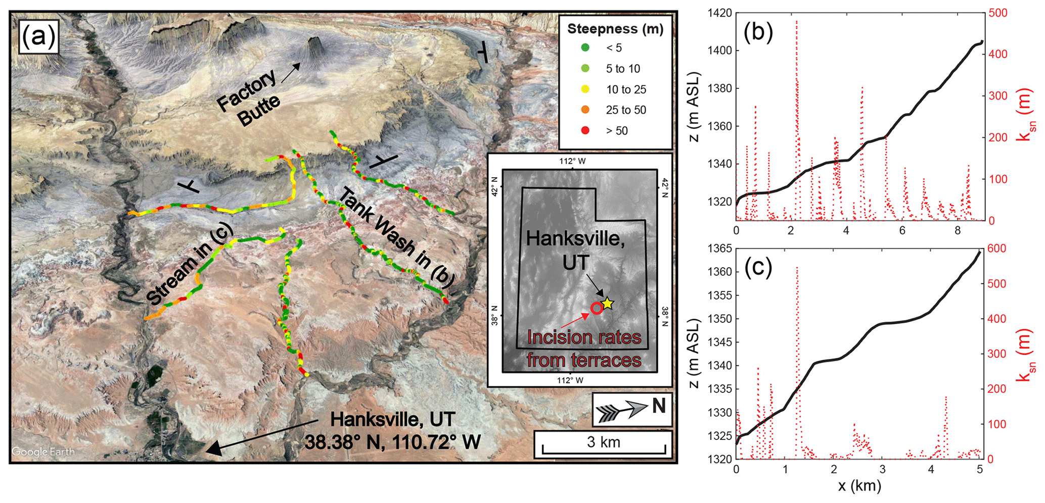
Figure 1Hanksville, UT, is a potential example of a landscape where contact migration significantly influences channel morphology. (a) Google Earth imagery (© Google Earth) showing variations in channel steepness (ksn using a reference concavity of 0.5) near Hanksville. These steepness values were obtained using TopoToolbox v2 (Schwanghart and Kuhn, 2010; Schwanghart and Scherler, 2014); more details regarding the extraction of profile data are available in Sect. S1. The inset shows the locations of Hanksville, UT (yellow star), and the fluvial terraces along the Fremont (red circle) that provide incision rate estimates of 0.3 to 0.85 mm yr−1 (Repka et al., 1997; Cook et al., 2009).
Figure 2 shows several conceptual models for bedrock river incision through layered stratigraphy. We have based these conceptual models on previous work (Perne et al., 2017; Darling et al., 2020) and present them to help guide the reader's understanding of this study's focus. Clearly, more complicated situations are likely in nature (e.g., a multitude of lithologies with variable thicknesses, contact dips that vary over space), but our intention here is to present simple examples. In Fig. 2a, we show the river reaches underlain by rock type 2 to be steeper than those underlain by rock type 1. Conventionally, this contrast would lead geomorphologists to suspect that rock type 2 has a higher resistance to erosion than rock type 1. As we discussed above, however, reaches in rock type 2 may be steeper because they have higher erosion rates (Perne et al., 2017). Note that such variations in steepness due to rock strength contrasts could be misinterpreted as having a different driver (e.g., changes in base-level fall rates). Figure 2b shows the stream in Fig. 2a at a later time; the balance between ongoing uplift (or base-level fall) and river incision causes the contacts to gradually migrate upstream along the stream profile. In Fig. 2c, the units dip in the upstream direction (i.e., a negative contact dip). In this case, the contacts will continue to migrate upstream but the magnitude of channel slope relative to contact slope varies along the profile. As a result, the influence of contact migration on erosion rates will vary along the profile (Darling et al., 2020). This consequence also applies to the river in Fig. 2d, which is underlain by units dipping in the downstream direction (i.e., a positive contact dip). Interestingly, when units dip in the downstream direction the contacts can migrate upstream or downstream. The direction of contact migration depends on the contrast between channel slope and contact slope (Darling et al., 2020). Importantly, in each conceptual model shown in Fig. 2 the spatial distributions of erosion rate, steepness, and contact migration rate all depend on incision model parameters such as erodibility (Perne et al., 2017; Darling et al., 2020). By understanding these landscapes, we may be able to capitalize on these effects and quantify erodibility in new ways.
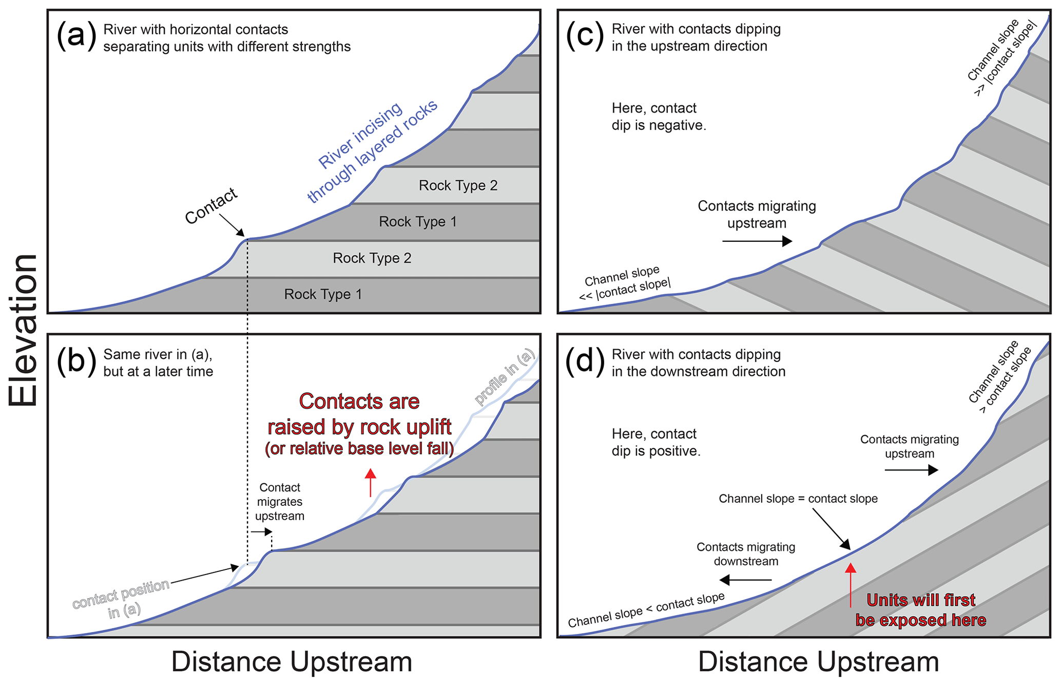
Figure 2Conceptual models of bedrock river incision through layered stratigraphy. Here, only two rock types are shown: rock type 1 and rock type 2. Panels (a, b) show a river with a contact dip (ϕ) of 0∘. Panel (b) is at a later time than panel (a) to demonstrate how the contacts gradually migrate upstream along the stream profile. Panel (c) shows a stream with contacts dipping in the upstream direction (ϕ<0∘). Panel (d) shows a stream with contacts dipping in the downstream direction (ϕ>0∘).
1.2 Research approach
In this contribution, we focus on how to use contact migration to gain insight into bedrock river behavior and quantify erodibility. Rather than being a complication to be avoided, the perturbation introduced by contact migration can be exploited for model calibration in a manner similar to how one would exploit a transient response to tectonics (Whipple, 2004). Although previous work has developed theories for bedrock river incision through layered rocks (Perne et al., 2017; Darling et al., 2020), these theories have not been thoroughly compared with observations from numerical models. Here, we use numerical models with which we can measure contact migration over time to pursue the following research questions: (1) does the theory developed by Perne et al. (2017) for river incision through horizontal strata accurately reflect observations from numerical models? (2) Does the theory developed by Darling et al. (2020) for river incision through nonhorizontal strata accurately reflect observations from numerical models? (3) What is the potential for using these theoretical frameworks to estimate incision model parameters like erodibility for real bedrock rivers? By developing a new method for estimating kinematic wave speed, we will show that morphologic metrics like steepness and contact dip can be used to estimate bedrock erodibility, even where contact dips are nonzero. The dynamics of landscapes with layered rocks are increasingly shown to be quite rich (Glade et al., 2017; Ward, 2019; Sheehan and Ward, 2020a, b), and these landscapes offer valuable opportunities to compare expectations shaped by model results with the unflinching testimony of the field. Our intention here is to (1) further elucidate what we should expect from the common form of the stream power model and (2) provide a framework for quantifying rock strength from bedrock river morphology. After developing this framework through the use of numerical models, we demonstrate its application on Tank Wash, one of the streams near Hanksville, UT (Fig. 1).
To address the research questions outlined above, we model one-dimensional river profiles using the stream power equation. We set up a series of model experiments to expand upon previous work and generate a framework for extracting quantitative information about erodibility in areas with complex lithology. Table 1 summarizes the numerical model scenarios we explore. We detail these models further below, but at this point we emphasize that we examine four distinct model scenarios: (1) models with two rock types and horizontal contacts; (2) models with three rock types and horizontal contacts; (3) models with two rock types and contacts dipping in the upstream direction; and (4) models with two rock types and contacts dipping in the downstream direction. We use the first two model scenarios to test and further explore the framework developed by Perne et al. (2017) (i.e., bedrock river incision through layered rocks when the contact dip is zero), and we use the last two model scenarios to test and further explore the framework developed by Darling et al. (2020) (i.e., bedrock river incision through layered rocks when contact dips are nonzero). Note that both studies are pertinent to river incision through horizontal or nonhorizontal units; we further describe in Sect. 2.4 why we focus on a particular application for each study's work.
Table 1Parameter space of the four model scenarios.
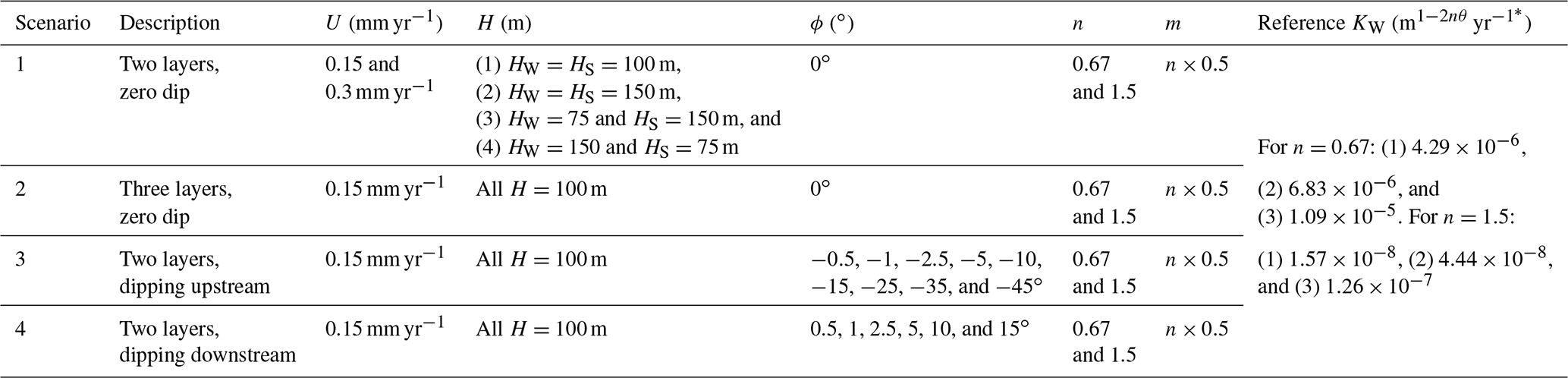
* The erodibilities of the medium layer (KM, only present in scenario 2) and strong layer (KS, present in all scenarios) are set relative to the reference weak erodibility (KW), as discussed in Sect. 2.2. We use θ=0.5 in the main text but present examples with θ=0.3 and θ=0.7 in the Supplement.
2.1 Bedrock river erosion and morphology
In this section, we present the basics of bedrock river erosion and the morphologic metrics we use to study it. We use a first-order upwind finite-difference scheme to represent the stream power model (Howard and Kerby, 1983; Whipple and Tucker, 1999):
where z is elevation (L), t is time (T), U is rock-uplift rate L T−1), E is erosion rate (L T−1), K is erodibility (L1−2m T−1), A is drainage area (L2), x is distance upstream (L), and both m and n are exponents. These exponents reflect erosion physics and the scaling of both channel width and discharge with drainage area (Whipple and Tucker, 1999; Lague, 2014). The ratio of has been shown to influence river concavity (θ) at steady state and uniform rock-uplift and erodibility (Tucker and Whipple, 2002). We use , which falls within the expected range of values (Whipple and Tucker, 1999) and is consistent with many other studies (Farías et al., 2008; Gasparini and Whipple, 2014; Han et al., 2014; Mitchell and Yanites, 2019). We present simulations using values of 0.3, 0.5, and 0.7 in the Supplement, however. Because slope exponent n strongly influences bedrock river dynamics (Tucker and Whipple, 2002), we evaluate n values of 0.67 and 1.5. Although n is often assumed to equal 1 (Farías et al., 2008; Fox et al., 2014; Goren et al., 2014; Ma et al., 2020), we explain in Sect. 2.4 why we do not evaluate models with n=1.
For an equilibrated stream () with uniform properties, channel steepness ksn is related to the ratio of rock-uplift rates to erodibility (Hack, 1973; Flint, 1974; Duvall et al., 2004; Wobus et al., 2006):
Equation (2) has shaped the focus of many studies in tectonic geomorphology (Wobus et al., 2006). Although this framework is powerful, the streams we examine here have spatially variable properties (i.e., K=f(x)). This distinction will cause variations in channel slope and steepness that are not captured by Eq. (2), and we seek to further understand these variations in slope and channel steepness.
We use Hack's law (Hack, 1957) to set each river's drainage area:
where x is distance upstream from the stream's outlet, ℓ is the length of the drainage basin (taken as 20.6 km), C is a coefficient (L2−h), and h is an exponent. We use C and h values of 1 m0.2 and 1.8, respectively. All streams are 20 km long, so using ℓ=20.6 km makes the rivers have a maximum drainage area of about 58 km2. This ℓ value also causes the critical drainage area (0.1 km2) to occur where x=20 km. We use a distance between stream nodes of dx=5 m.
We present the resulting stream profiles as χ plots here because χ–z space removes the influence of drainage area on channel slope (Perron and Royden, 2013; Mudd et al., 2014):
where χ is transformed distance upstream (L), xb is the position of base level (x=0 m), and A0 is a reference drainage area (here, taken as 1 km2).
An effective method for comparing channel slopes and contact dip ϕ is to use the slope of the contact in χ space, which we refer to as ϕχ:
where zcontact is contact elevation (L) and χ is that of the stream node directly above the contact position in question. Admittedly, comparing contact elevations with χ may be initially confusing, as χ is related to river elevations rather than contact elevations. Utilizing the apparent contact dip in χ space is advantageous, however, because it encapsulates the influence of both drainage area and contact dip in real space. If one decides to utilize only drainage area or contact dip, then the influence of the excluded metric would not be present in one's analyses. Note that we will present ϕχ as dimensionless values (i.e., the change in elevation over the change in transformed river distance), while we present contact dip ϕ in degrees.
2.2 Defining the range of erodibility values
The contrast in erodibility (K) values between weak and strong layers is one of the most important controls on bedrock river incision through layered stratigraphy, and we therefore explore this parameter space thoroughly. Selecting K values for different simulations is not a simple matter, however. The way erodibility influences river dynamics depends on the exponents m and n, so the effects of a 2-fold difference in K on both stream morphology and erosion dynamics is not the same for n=0.67 and n=1.5. Furthermore, comparing K values is context-dependent. For example, K values could be selected to either (1) provide a similar range of channel elevations (Beeson and McCoy, 2020) or (2) allow similar timescales for transient adjustment (Mitchell and Yanites, 2019). Oftentimes, one cannot fulfill multiple such requirements when selecting erodibilities and one must choose a specific approach. Because we examine different n values here, we set the range of erodibility by considering slope patch migration rates (Royden and Perron, 2013).
For the sake of concision, we summarize our approach for setting erodibility values in Sect. S2. We use three reference weak erodibilities (KW) for each n value (Table 1). Using these references KW values, we then calculate the erodibility for the stronger layer (KS) so it produces slope patch migration rates that are a certain fraction (33 %, 50 %, 67 %, 75 %, or 90 %) of those calculated for the weaker layer. We chose this approach because (1) it allows us to objectively and thoroughly explore K contrasts between weak and strong layers, and (2) the approach is consistent even with changes in slope exponent n. While the erodibilities we use for different m and n values vary over several orders of magnitude, K values corresponding to different drainage area m values have different dimensions (L1−2m T−1) and therefore cannot be directly compared. The K values we use are comparable to those reported by Armstrong et al. (2021) (for those with the same m values).
2.3 Recording contact migration rates
We tracked and recorded contact positions over time in our simulations. We recorded each contact's position every 25 kyr, which is larger than model time step dt=25 yr. Contact migration rates are recorded for a total of 10 Myr for each simulation. Note that before we begin recording contact migration rates, we run each simulation for a time period sufficient to allow the range of river elevations to become constant over time (i.e., a state of dynamic equilibrium). When n<1, we initialized the river elevations using the steepness (Eq. 2) for steady conditions and the strong layer's erodibility (). When n>1, we initialized the river elevations using the steepness for steady conditions and the weak layer's erodibility (). After we initialized the river elevations, the rivers needed some time to adjust from the initial conditions. Although the rivers quickly arrive at morphologies like those shown in our conceptual model (Fig. 2), the river elevations can gradually increase or decrease before finally arriving at a consistent range of elevations (Figs. S1–S4 in the Supplement). The required adjustment duration depends on both the initial conditions and the rock-uplift rate used (i.e., the time for a contact to be uplifted across the fluvial relief). Streams in scenarios 1, 2, and 4 (Table 1) were given 50 Myr to adjust, while streams in scenario 3 were given 100 Myr to adjust. These adjustment times ensured that the streams in all simulations had achieved a dynamic equilibrium (i.e., the range of elevations became constant with time; Figs. S1–S4). We discuss our approach for measuring contact migration rates in our models in Sect. S3.
2.4 Erosion and kinematic wave speed for horizontal units
Now, we delve further into (1) the erosion rate variations that occur during river incision through layered stratigraphy and (2) how these erosion rate variations influence kinematic wave speed. We will show that kinematic wave speed is an important concept for this research because it is closely linked to contact migration along rivers. In this section, we review the semi-analytical framework developed for kinematic wave speed when contact dip is zero (Perne et al., 2017).
Before we outline the semi-analytical framework developed in previous work, we provide a background on how erosion rate relates to kinematic wave speed. Contact migration can cause the erosion rates on either side of a contact to change (Perne et al., 2017; Darling et al., 2020). One side of the contact can have an erosion rate below the base-level fall rate, while the other side can have an erosion rate above it. These erosion rate variations occur so that both sides of the contact have the same horizontal retreat rate in the upstream direction. This retreat rate is closely related to the concept of kinematic wave speed (CH) (Rosenbloom and Anderson, 1994):
Note that Eq. (6) suggests that CH has a power-law relationship with drainage area (A). Although this is the general equation for kinematic wave speed, the challenge when considering rivers incising through layered rocks is what erosion rate E is appropriate. Kinematic wave speed can be regarded as the migration rate of signals along rivers. When considering such signals, geomorphologists usually think of base-level fall due to tectonic activity (e.g., normal faulting) or drainage capture. The signals we are concerned with here, however, are the erosional signals arising from contact migration. Because the exposure of a new rock type can perturb erosion rates (Forte et al., 2016), even without changes in external drivers like base-level fall rate and climate, contact migration is an autogenic perturbation. As erosion causes a contact to migrate upstream along a river, the autogenic signal persists and becomes a significant influence on river morphology.
Perne et al. (2017) showed that when contacts are horizontal (ϕ=0∘), river reaches underlain by weak and strong rock types will have characteristic steepness values that reflect the layers' relative difference in erodibility. Surprisingly, the steeper reaches can sometimes be within the weaker rock type. Whether reaches in the strong or weak rock type are steeper depends on n, the parameter that controls how erosion rate scales with channel slope (Eq. 1). The slope exponent n plays an important role in bedrock river incision through layered stratigraphy because it controls how kinematic wave speed scales with erosion rate (Eq. 6). The nonlinearity of Eq. (6) increases with . When n>1, CH is directly proportional to E. When n<1, CH is inversely proportional to E. And when n=1, CH is independent of E. Strangely, this insensitivity of CH to E when n=1 causes channels incising through layered rocks to consist only of flat reaches and vertical steps (Fig. S5). The channel slopes when n=1 are either infinite or zero (infinite at the steps and zero in the flat reaches). Although this morphology has been compared with waterfalls (Perne et al., 2017), waterfall dynamics are quite distinct (Lamb et al., 2007; Haviv et al., 2010; Scheingross and Lamb, 2017) and require a different treatment. We do not intend to explicitly portray waterfalls here, and we therefore focus on models with n values of 0.67 and 1.5. We also do not assess simulations with n=1 because we argue that Eq. (6) is not representative for those conditions. When n<1, the weaker rock type has higher channel slopes and erosion rates (Perne et al., 2017). Conversely, when n>1 the strong rock type has higher channel slopes and erosion rates. We will use observations from our numerical models to further demonstrate why these behaviors emerge.
Because river incision through layered rocks in highly dependent on slope exponent n, simply evaluating the ratio of the weak and strong layers' erodibilities () is not an effective way to encapsulate the influence of contact migration. Instead, we use a term that is a function of the weak and strong erodibilities as well as slope exponent n. Darling et al. (2020) showed that if you consider weak and strong rock types (with kinematic wave speeds and , erodibilities KW and KS, steepness values and , and erosion rates EW and ES, where the subscripts refer to weak and strong layers, respectively) and set the kinematic wave speeds equal to one another, you arrive at an equation Perne et al. (2017) derived through a different approach. Because many readers will be unfamiliar with this work, we show the derivation in three parts.
We refer to this ratio as K*. Note that if you express and in Eq. (7c) using Eq. (2) (e.g., , you will also find that
where EW and ES are the erosion rates in the weak and strong layers, respectively. Even though K* represents the contrast in erosion or steepness between weak and strong rock types when the contact dip is zero, we will show that K* is still an effective metric for erodibility contrasts when contact dips are nonzero (in the form (). Although we focus on the approach of Darling et al. (2020) for nonzero contact dips, it can be applied to river incision through horizontal units (by setting the contact slope to zero). The approach of Darling et al. (2020) then becomes the same as that of Perne et al. (2017) (i.e., both studies derived Eq. 7c), however, so we focus on the work of Darling et al. (2020) for nonzero contact dips. Although Darling et al. (2020) derived K* by considering kinematic wave speeds, Perne et al. (2017) derived K* by assuming that
where ϕ is the contact dip in degrees (positive when dipping in the downstream direction). The concept behind this approach is that if the contact dip is high (e.g., vertical contacts that do not migrate horizontally), the right side of Eq. (9) approaches 1. In that case, rearranging the equation would return us to the general expectations formed without considering contact migration: that the erosion rate is the same within each rock type (). If, however, the channel slopes are much higher than the contact slopes, then ϕ can be considered to go to zero. If ϕ=0∘, replacing the erosion rates in Eq. 9 with the stream power equation (Eq. 1) and rearranging leads to K* (Eq. 7c). A similar approach was used by Imaizumi et al. (2015), albeit for the retreat of rock slopes rather than rivers.
The semi-analytical framework presented by Perne et al. (2017) can be used to calculate kinematic wave speeds for bedrock rivers incising through horizontal strata. We use measurements from our numerical models to test the accuracy of predictions made with their framework. To calculate the kinematic wave speed for a reach underlain by a strong layer, one must first solve for the erosion rate as (Perne et al., 2017)
where ES is the erosion rate in the stronger layer (L T−1), and HS and HW are the layer thicknesses (L) of the strong and weak layers, respectively. To calculate the weak erosion rate (EW) for a contact dip of zero, the strong and weak indices in Eq. (10) can simply be reversed. The kinematic wave speed within one layer can then be estimated by inserting Eq. (10) into the general equation for kinematic wave speed (Eq. 6). Note that Perne et al. (2017) derived Eq. (10) by assuming that the average erosion at each point along the stream over time must balance the rock-uplift rate (U). To understand the concept behind this approach, first consider a reach that is underlain by one rock type and that is eroding at a rate above U. As erosion causes the contacts defining that reach to migrate upstream over time, the reach creates an imbalance between the river's erosion rate and rock-uplift rate. After the reach migrates past one position, however, its migration is followed by a reach in another rock type. This rock type would have an erosion rate below the rock-uplift rate, and the passage of this low-erosion reach restores the balance over time between rock uplift and erosion. Perne et al. (2017) based this perspective on observations from their numerical models; despite oscillations in channel slope as contacts migrate upstream, the rivers reached a dynamic equilibrium such that the range of elevations was constant over time. This dynamic equilibrium suggests that erosion and rock uplift do balance each other over a sufficient time interval (i.e., the time for reaches in both rock types to migrate past a position). Given the assumptions involved in the derivation of Eq. (10), however, we will use measurements from our numerical models to test its accuracy.
To test if Eqs. (7)–(10) are accurate across different values, we also assess six additional simulations: two with , two with , and two with . For each value, the two simulations use n values of either 0.67 or 1.5. Because each simulation uses different m values, these simulations require a different approach for setting erodibility values. We discuss this approach in Sect. S4.
2.5 Erosion and kinematic wave speed for nonhorizontal units
When units have nonzero dips, the dynamics between erosion rate and kinematic wave speed change entirely (Darling et al., 2020). To evaluate how bedrock river erosion rates vary with contact dip, we fit multilinear regressions to our model results in the form
where is the average erosion rate of the weak unit normalized by rock-uplift rate, K* is a metric for the erodibility contrasts between weak and strong layers (Eq. 7c), and ϕχ is the contact dip in χ space (Eq. 5). The purpose of this approach is to demonstrate how erosion rates change with drainage area, contact dip (both of which influence ϕχ), and contrasts in rock strength. We take the average and values within 10 drainage area bins spaced logarithmically from the highest to lowest drainage areas. Utilizing the logarithm of is effective because this drainage area proxy aids in portraying the power-law relationships surrounding drainage area in the stream power model (Eq. 1). Excluding the influence of contact dip by using drainage area instead of would, for example, provide only scatter rather than the three-dimensional relationships we will demonstrate between , K*, and . For these analyses, we only use erosion rates from the final model time step (rather than values over the entire 10 Myr duration).
Now, we present the framework for kinematic wave speeds along bedrock rivers incising through nonhorizontal strata. Darling et al. (2020) used geometric considerations to solve for the kinematic wave speed as
where the weak layer is assumed to erode at rock-uplift rate U. Note that Eq. (12) suggests that when ϕ<0∘ (dipping upstream), CH will be lower (i.e., the denominator will increase). When ϕ>0∘ (dipping downstream), CH will be higher (i.e., the denominator will decrease). Although CH usually increases as a power-law function of drainage area (Eq. 6), Eq. (12) also suggests that nonzero contact dips will cause a departure from the power-law relationships typically expected (i.e., in a log–log plot of CH vs. drainage area, the data will no longer follow a linear trend). While Perne et al. (2017) showed that the erosion rate of the weak layer changes when contact dip is zero, Darling et al. (2020) assumed that the weak layer erodes at the base-level fall rate. Darling et al. (2020) focused on scenarios with n>1; because the strong layer is the less steep layer when n<1, we will use the parameters of the strong layer (KS) in Eq. (12) when n<1.
In addition to Eq. (12), we present an alternative method to estimate kinematic wave speed from channel steepness. We have essentially modified the approach of Darling et al. (2020) to utilize observed channel steepness. The approach remains applicable whether the contact dip is zero or nonzero, and although it utilizes a base-level rate (U) it is not based on assumptions regarding the erosion rate within each layer. Kinematic wave speed CH for a reach underlain by one rock type can be estimated as
where ksn is the average steepness observed for the reach spanning the layer in question. We estimate the K value in Eq. (13) as ; this approach assumes the reach is equilibrated to U and previous work (Forte et al., 2016; Perne et al., 2017; Darling et al., 2020) suggests that this assumption can be incorrect. The advantage of this approach, however, lies in taking the average of Eq. (13) estimates from multiple rock types. For example, the Eq. (13) CH estimates for one rock type will be too high, while the CH estimates for the other rock type will be too low. By taking the average of both estimates, the deviations in erosion rate balance each other out and provide an accurate estimate of CH. Importantly, this approach can then be combined with that of Darling et al. (2020) (Eq. 12). By utilizing Eqs. (12) and (13) together, one can compare CH estimates based only on quantifiable metrics (U, ksn, and ϕ in Eq. 13) and CH estimates calculated using a specified erodibility (Eq. 12). We will show that this combination can allow the estimation of erodibility for real streams, like those near Hanksville, UT (Fig. 1). We describe this combination further below, after we provide more details regarding the application of Eq. (13).
To estimate CH with Eq. (13), we utilize the following procedure: (1) create bins defined by drainage area values, with 10 bins spaced logarithmically from the lowest to the highest drainage areas; (2) for each drainage area bin, take the average steepness (ksn) within each rock type; (3) using the average steepness for each rock type, calculate CH with Eq. (13); and (4) take the average of the CH estimates from both rock types in each drainage area bin. Note that this approach requires an independent estimate of rock-uplift rate U (or base-level fall rate) and contact dip ϕ. Due to the data limitations for real streams, we will compare contact migration rates measured in our models with Eq. (13) CH estimates that use only ksn values from the final model time step of each simulation. We show Eq. (13) estimates using the entire 10 Myr of recorded ksn values for each simulation in the Supplement, however. Equation (12) does not use ksn values recorded over time. Note that we bin results by drainage area mainly for visual clarity in our figures. To test the influence of our binning approach, we present a figure in the Supplement in which we use 20 drainage area bins instead of 10.
To further examine the influence of different values, we also assess six additional simulations with a contact dip ϕ of −2.5, n values of 0.67 or 1.5, and values of 0.3, 0.5, or 0.7. The approach for setting erodibility values in these simulations is discussed in Sect. S4. Although we examine a wider range of contact dips in our main simulations (Table 1), these additional simulations are meant to be a limited selection of examples that demonstrate the influence of different values on bedrock river incision through layered rocks.
Now, we describe how we combine the framework developed by Darling et al. (2020) (Eq. 12) with our approach (Eq. 13) in the evaluation of our numerical models. Note that we perform this comparison to test how well it can recover erodibility values from river morphology in a numerical model; establishing this accuracy is important because we apply similar analyses to Tank Wash near Hanksville, UT (Fig. 1). We describe our analysis of Tank Wash in Sect. 2.6 below. To test the effectiveness of this approach in the numerical models, we compare the average Eq. (13) CH estimate within each drainage area bin with Eq. (12) CH values calculated using the enforced contact dip (ϕ) and slope exponent (n) as well as a wide range of erodibilities (K, 200 values spaced logarithmically from 10−9 to 10−4 m1−2nθ yr−1, where θ=0.5). We compare the two sets of kinematic wave speed estimates with the X2 misfit function (Jeffery et al., 2013):
where N is the number of observations being compared (up to 10 for average values in the 10 drainage area bins), ν is the number of free variables (ν=1 here, as we only vary K in Eq. 12), simi and obsi are the CH estimates from Eqs. (12) and (13) in each drainage area bin, respectively, and “tolerance” is taken as 1 m yr−1. Note that we take the obsi values as the average CH estimates made with Eq. (13); we made this decision because (1) CH values from Eq. (13) are based on measured steepness, (2) we thoroughly compare our Eq. (13) estimates with contact migration rates measured in our models, and (3) measured contact migration rates would not be available for a real stream. Although tolerance can be set in such a way that simulations with X2 values under some threshold are defined as acceptable, we do not use X2 in that manner here. Instead, we show the X2 values for all Eq. (12) estimates (using 200 K values spaced logarithmically from 10−9 to 10−4 m1−2nθ yr−1) and focus on the K with the lowest X2 as the best-fit K (i.e., this would be the best estimate for the stream's erodibility). Varying the tolerance would scale the magnitudes of all X2 values, but it would not alter which K value corresponds to the lowest X2. We compare the best-fit K values in each simulation with the simulation's weak and strong erodibilities (KW and KS).
Although we use this approach to search for the K value that produces the best agreement between the Eq. (12) and (13) estimates of CH (the Eq. 12 estimates use a range of K and the Eq. 13 estimates use measured ksn), we do not perform such a search for the slope exponent n value. In each simulation, we calculate Eq. (12) and (13) estimates of CH using the n value enforced in each simulation. Using the correct m and n values is crucial for estimating the appropriate magnitude and dimensions of erodibility, but our intention here is only to show how accurately K can be estimated. Using the incorrect n to estimate the K used in a simulation would involve comparing erodibilities with different dimensions (if remains constant). As we discussed in Sect. 2.2, comparing K values is context-dependent. We could compare the fluvial relief values expected for different K, or we could compare slope patch migration rates. Attempting to fully explore such considerations, however, would negatively impact the focus and brevity of this study. Furthermore, we perform these analyses on our numerical models to inform our analysis of Tank Wash (Sect. 2.6), and our analysis of Tank Wash includes the consideration of multiple n values.
2.6 Analysis of Tank Wash
We explore the behavior of these rivers in numerical models to develop a framework for quantifying erodibility from bedrock river morphology. After presenting our numerical model results, we apply the developed framework to Tank Wash near Hanksville, UT (Fig. 1). We use Google Earth imagery and the nearby 1:62k geologic map of the San Rafael Desert Quadrangle (which includes the same units; Doelling et al., 2015) to infer the map-view positions of contacts near Tank Wash. We then infer the contact locations along Tank Wash's longitudinal profile by considering both the inferred map-view contacts and changes in the stream's steepness (Fig. 1b). Channel profile data are taken from 10 m digital elevation models (DEMs) provided by the United States Geological Survey. We extracted profile data using TopoToolbox v2 (Schwanghart and Kuhn, 2010; Schwanghart and Scherler, 2014); more details regarding the extraction and processing of profile data are available in Sect. S1 in the Supplement. There are no contact dip measurements available in the vicinity of Tank Wash, but based on regional geology, the contact dips are likely relatively low. For example, Ahmed et al. (2014) reported a dip of 3∘ to the west in an area just north of Tank Wash. We evaluate contact dips of −1 and −5∘ (dipping in the upstream direction) because the geologic maps (Doelling et al., 2015) and imagery available in the area suggest that contact dips are likely relatively low. Furthermore, our results will demonstrate the effect of contact dip on these analyses in a manner that enables extrapolation (e.g., considering if the dip was −3 or −10∘). Although this approach is far from ideal, our intention here is only to demonstrate how one could apply the developed framework to real streams. Any accurate analyses would require detailed field surveys, and such endeavors could be the focus of future work.
After identifying the potential contacts, we (1) divide Tank Wash's profile into reaches separated by the inferred contact locations and (2) use the average steepness of each reach to estimate kinematic wave speed (CH) values according to Eq. (13). These CH estimates are made twice for each reach: once at the minimum drainage area and once at the maximum. We then take the average of all CH values within five drainage area bins spaced logarithmically from the lowest to highest drainage areas. To explore what erodibilities could yield similar results (given the assumed contact dips evaluated), we compare the average CH estimates from our approach (Eq. 13) with a range of predictions from the Darling et al. (2020) portrayal of kinematic wave speed (Eq. 12). We perform this comparison with the X2 misfit function (Eq. 14). We evaluate a large range of K for Tank Wash (200 values spaced logarithmically from 10−8 to 10−2 m1−2nθ yr−1, where θ=0.5). Because Eq. (12) requires an estimated rock-uplift rate (i.e., base-level fall rate), we use the range of incision rates from the cosmogenic dating of fluvial terraces along the nearby Fremont River (0.3 to 0.85 mm yr−1; Repka et al., 1997; Cook et al., 2009; red circle in Fig. 1a). Incision rates from terraces are not necessarily representative of base-level fall rates, but there are no other constraints in the area. Importantly, our results will enable us to consider how the estimated erodibility would scale with the assumed base-level fall rate (i.e., considering how the erodibility would change if the incision rate was only 0.15 mm yr−1 instead of 0.3 mm yr−1). For this analysis of Tank Wash, we evaluate n values of 0.67 and 1.5 and assume that . Although a wide range of n values are possible, our intention is to focus on a limited number of examples for which n is less than or greater than 1. Similarly, the example simulations that use different values (Sect. S4) will allow us to consider the influence of varying .
3.1 Scenario 1: two rock types with ϕ=0∘
In this section, we present the results for scenario 1 of our numerical models (Table 1). These simulations use two rock types (weak and strong) with contact dips of 0∘. We use the results for scenario 1 to (1) further explain the dynamics of bedrock river incision through flat-lying strata and (2) test and further explore the semi-analytical framework developed by Perne et al. (2017).
Figure 3 shows long profiles (Fig. 3a and b) and χ plots (Fig. 3c and d) for two simulations of bedrock rivers underlain by alternating weak and strong rock layers. The simulation in Fig. 3a and c has n=0.67 and K* of ∼9.5 (weak layer's erodibility K is ∼2.1 times higher than the strong layer's K), while the simulation in Fig. 3b and d has n=1.5 and K* of ∼0.13 (weak layer's K is ∼2.8 times higher than the strong layer's K). Note that the erosion rates normalized by rock-uplift rate () are shown as red lines. Like the streams near Hanksville, UT, and those simulated by Perne et al. (2017), these streams have a stepped appearance. As we discussed in Sect. 2.4, when n<1 (Fig. 3a and c) reaches underlain by the weaker rocks have higher channel slopes and erosion rates. When n>1 (Fig. 3b and d), reaches underlain by the stronger rocks have higher channel slopes and erosion rates. To explain why the erosion rate variations in Fig. 3 occur, we now examine the contact migration rates within each of these simulations.
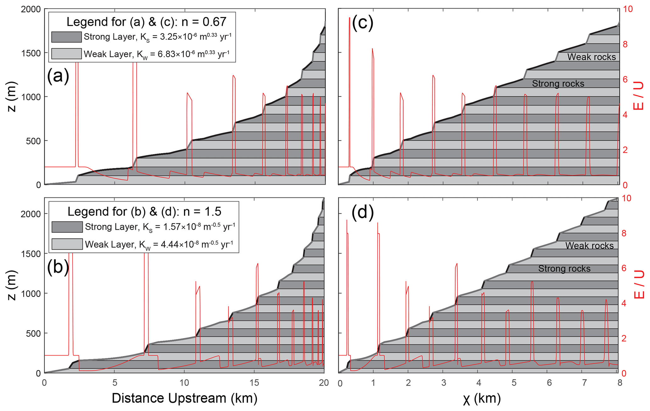
Figure 3Longitudinal profiles (a, b) and χ plots (c, d) for two different simulations. The simulation in (a) and (c) has slope exponent n values of 0.67, while the simulation in (b) and (d) has n=1.5. Layer thickness H and rock-uplift rate U are 100 m and 0.15 mm yr−1 in both simulations, respectively.
Figure 4a and b show contact migration rates (ddt) versus drainage area (A) for the simulations in Fig. 3a and b, respectively. We show the average measured contact migration rates (gray circles with black outlines) within 10 drainage area bins; the vertical bars for each circle represent the standard deviation of ddt within the corresponding drainage area bin. In Fig. 4a and b, the light gray dotted line represents the kinematic wave speed (Eq. 6) expected if only the weak layer was present and all erosion rates were equal to the rock-uplift rate. Similarly, the dark gray dashed line shows the kinematic wave speed expected if only the strong layer was present and all erosion rates were equal to the rock-uplift rate. If only one rock type was present, one could think of these wave speeds as the upstream migration rate of bedding planes within the units, as rock uplift carries the units up the stream profile. The measured contact migration rate lies somewhere between these two end-members. This finding is highlighted by the dashed red lines, which are power-law functions fit between the observed contact migration rates and the drainage areas at the center of each bin (assuming a drainage area exponent of , which is 0.5 here). While the fact that contact migration rates fall between the two extremes shown in each panel may sound straightforward, the reason for this result is not intuitive.
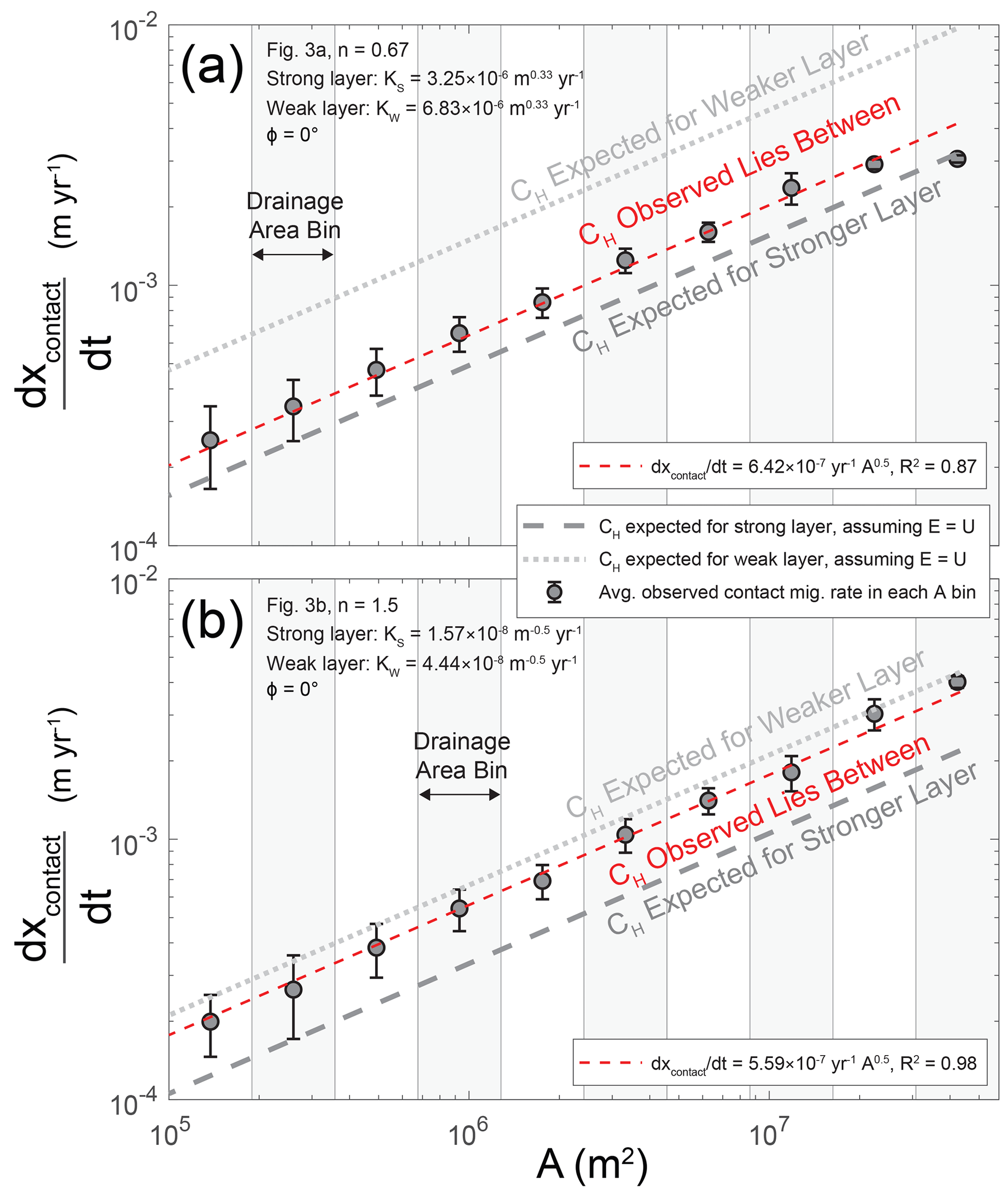
Figure 4Contact migration rates (ddt) vs. drainage area (A) for (a) the simulation shown in Fig. 3a and c and (b) the simulation shown in Fig. 3b and d.
These dynamics occur because channel slopes on both sides of the contact interact to drive the system towards equal retreat rates and kinematic wave speeds (CH) across the contact. For example, consider a contact with a weak unit situated beneath a strong unit. The stream segment in the weak unit may initially erode at a higher rate, undercutting the strong unit and forcing the contact further upstream. Importantly, the response of the strong unit depends on slope exponent n in the stream power model. When n>1, higher erosion rates in the weak unit will cause a consuming knickpoint (Royden and Perron, 2013) to migrate into the strong unit situated above. The strong unit responds rapidly in this case, keeping pace with the weak unit by eroding at a higher rate. This response is so effective that the contact's migration leads to a reduction in channel slope within the weak unit (i.e., lengthening each reach within the weak unit), decreasing the weak unit's erosion rate. When n<1, however, there is no consuming knickpoint. Instead, the initially higher erosion rate in the weak unit causes an erosional signal that migrates more slowly through the strong unit above. A stretch zone (Royden and Perron, 2013) initially forms at the base of the strong unit (i.e., a convex-upwards knickzone). Instead of rapidly adjusting to keep pace with the weak unit, in this case the strong unit slows down the contact's migration. The stretch zone in the strong unit is then replaced by a reach of low steepness. This transition occurs because the combination of undercutting by the weak unit and resistance from the strong unit leads (1) to higher channel slopes and erosion rates within the weak unit and (2) lower channel slopes and erosion rates within the strong unit (i.e., due to lengthening of each reach within the strong unit).
Although we discussed these dynamics in qualitative terms above, we will now we discuss them with a stronger focus on contact migration rates (Fig. 4) and kinematic wave speed (CH). To maintain equal retreat rates, reaches within the weaker layer develop a lower CH value relative to what would be expected if they were eroding at the rock-uplift rate (dotted gray lines in Fig. 4). Conversely, reaches within the stronger layer develop a higher CH value. When n<1, Eq. (6) shows that CH is inversely proportional to erosion rate E. Because of this relationship, reaches in the weak layer achieve a lower CH (i.e., slow down) by increasing E when n<1. Similarly, reaches in the strong unit achieve a higher CH (i.e., speed up) by decreasing E when n<1. Due to such behaviors, when n<1 the stream has higher steepness and erosion rates within the weak unit and subdued steepness and erosion rates within the strong unit. The opposite is true when n>1; reaches in the weak unit obtain a lower CH value (i.e., slow down) by decreasing E, and reaches in the strong unit obtain a higher CH value (i.e., speed up) by increasing E.
To assess if the theory developed by Perne et al. (2017) is applicable across the parameter space explored in scenario 1, we compared kinematic wave speeds calculated with Eqs. (6) and (10) with contact migration rates (ddt) measured in our models (Fig. 5). Note that in Fig. 5, both metrics have been normalized by drainage area raised to the ; as shown in Fig. 4, contact migration rates change with drainage area. Despite all of the changes in parameters like erodibilities, layer thicknesses, and rock-uplift rates in scenario 1 (Table 1), the kinematic wave speeds predicted using the framework from Perne et al. (2017) (Eqs. 6 and 10) serve as excellent portrayals of the contact migration rates in our numerical models. These findings indicate that when contacts are horizontal, contact migration rates reflect the kinematic wave speeds of the surrounding stream reaches. Furthermore, erosion rate variations like those in Fig. 3 occur so that kinematic wave speeds are equal on either side of a contact, allowing kinematic wave speed to consistently increase with drainage area as shown in Fig. 4.
Figures S6–S10 show the results for the six additional simulations with horizontal contacts and different values (0.3, 0.5, or 0.7). Even though the dimensions of erodibility depend on m, which varies across these simulations (Figs. S6 and S7), the simulations with the same n value (0.67 or 1.5) were set up to have the same K* value. Because the simulations have the same K* value, the variations in erosion rate are roughly the same. These findings suggest that the nondimensional parameter K* is representative of the variations in channel steepness and erosion rate caused by rock strength contrasts (Eqs. 7c, 8, and 10) even when drainage area exponent m varies. Furthermore, the contact migration rates measured in these additional simulations are still well represented by the kinematic wave speeds calculated with the framework of Perne et al. (2017) (Fig. S10).
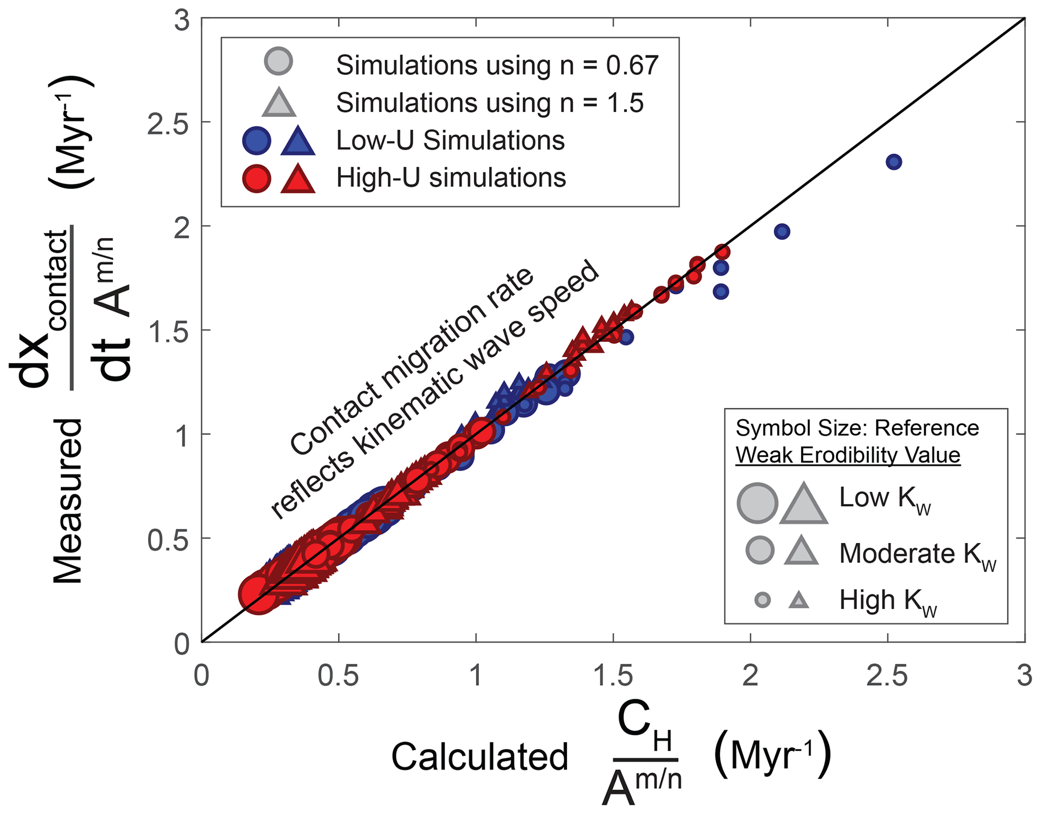
Figure 5Estimated kinematic wave speeds (CH) and measured contact migration rates (ddt) for all simulations in scenario 1 (Table 1). The low-U scenarios have U=0.15 mm yr−1, while the high-U scenarios have U=0.3 mm yr−1. Symbol size represents the reference weak erodibility used (KW; Table 1).
3.2 Scenario 2: three rock types with ϕ=0∘
In this section, we examine the results for scenario 2 (Table 1). Like scenario 1, scenario 2 only considers horizontal contacts (contact dip ϕ=0∘). Unlike scenario 1, however, scenario 2 utilizes three rock types (weak, medium, and strong). Our intention is to test if the equations presented by Perne et al. (2017) still hold when there are more than two rock types because real streams usually incise through strata that are far more complicated than those considered in scenario 1.
Figure 6a and b show long profiles with three rock types of equal thickness (100 m) and n values of 0.67 (Fig. 6a) and 1.5 (Fig. 6b). Figure 6c shows ratios of the average steepness values (ksn) and erosion rates (E) within different rock types (e.g., ksn of weak layer ksn of strong layer) for all simulations in scenario 2. The purpose of Fig. 6c is to test if Eqs. (7c) and (8) (Perne et al., 2017) are still accurate when there are three rock types instead of two. Because the steepness and erosion ratios in Fig. 6c follow a 1:1 relationship with K*, these results are consistent with Eqs. (7c) and (8).
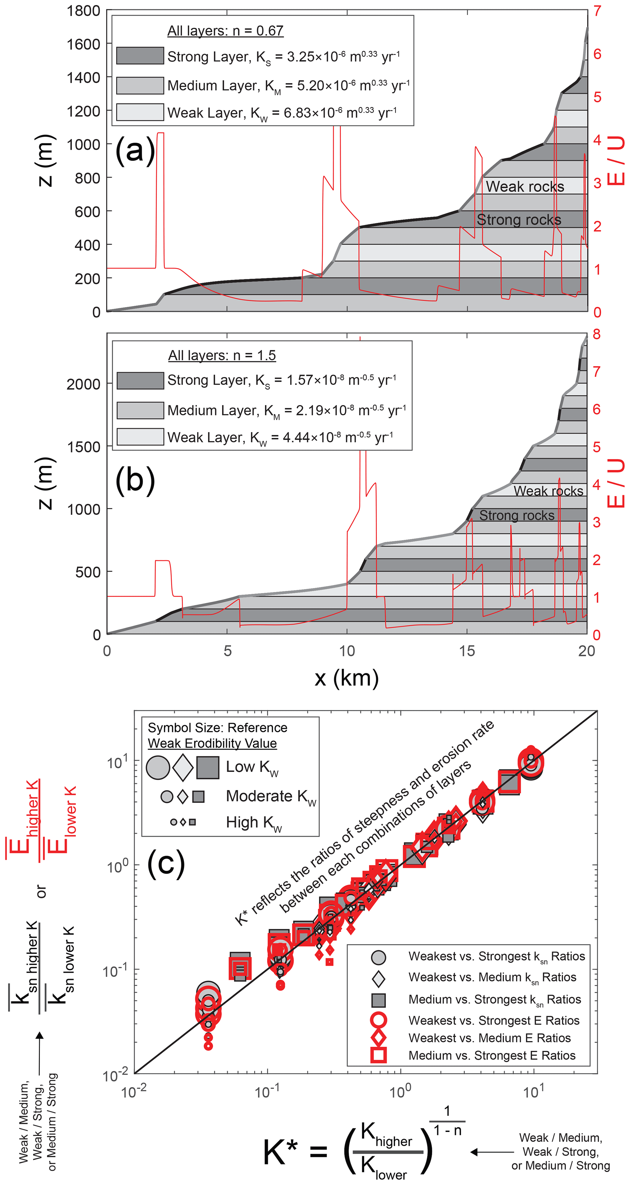
Figure 6Longitudinal profiles (a, b) for two simulations using three rock types. The scenario in (a) has n=0.67, while the scenario in (b) has n=1.5. (c) Ratios of steepness ksn and erosion rate E for all simulations in scenario 2 (Table 1).
These results suggest that the theory developed by Perne et al. (2017) for bedrock river incision through horizontal strata still applies when there are more than two rock types. When there is an additional rock type (e.g., more than three lithologies), the channel slopes and erosion rates within the additional rock type will adjust to allow for a consistent trend in kinematic wave speed across the profile. Here, the medium layer is the additional rock type relative to the simulations in scenario 1. For example, Fig. S11 shows the contact migration rates for the simulations in Fig. 6a and b; despite differing erodibilities, contact migration rates and CH increase as a power-law function of drainage area. The fact that steepness ratios and erosion rate ratios are both well represented by K* (Fig. 6c) follows from Eqs. (7c) and (8), which were derived by setting the kinematic wave speeds within two rock types equal to each other.
3.3 Scenarios 3 and 4
3.3.1 General morphologic results of nonzero contact dips
Before we test the framework developed by Darling et al. (2020) for bedrock river incision through nonhorizontal strata, we present example simulations demonstrating the general morphologic implications of nonzero contact dips. Our simulations indicate that river morphology can be significantly altered by even slight changes in contact dip (Figs. 7 and 8). Figure 7 shows the long profiles (Fig. 7a and b) and χ plots (Fig. 7c and d) for two simulations with n=0.67 and the same erodibility values (K) used in Fig. 3a, but with slight dips to the contacts. One simulation has contacts dipping upstream at 2.5∘ (∘; Fig. 7a and c), and the other simulation has contacts dipping downstream at 2.5∘ (ϕ=2.5∘; Fig. 7b and d). Although the strong and weak erodibilities in Fig. 7 are the same as those in Fig. 3a, the morphologies of these streams are quite distinct. For example, although the simulations use the same erodibilities, rock-uplift rates, layer thicknesses, and drainage areas, the maximum river elevations in Figs. 3a, 7a, and 7b are about 1800, 2300, and 1700 m, respectively. Indeed, such pronounced changes in river erosion and morphology for deviations in contact dip of only 2.5∘ away from horizontal bedding planes highlight the importance of contact dip in river morphology. Note that in the χ plots in Fig. 7, the apparent contact dip in χ space (ϕχ; Eq. 5) varies along the profile. When contacts dip upstream (ϕ<0∘) ϕχ is negative, and when contacts dip downstream (ϕ>0∘) ϕχ is positive. In both χ plots, however, the absolute value of ϕχ approaches zero with increasing χ (i.e., the contacts seem to bend and almost become horizontal).
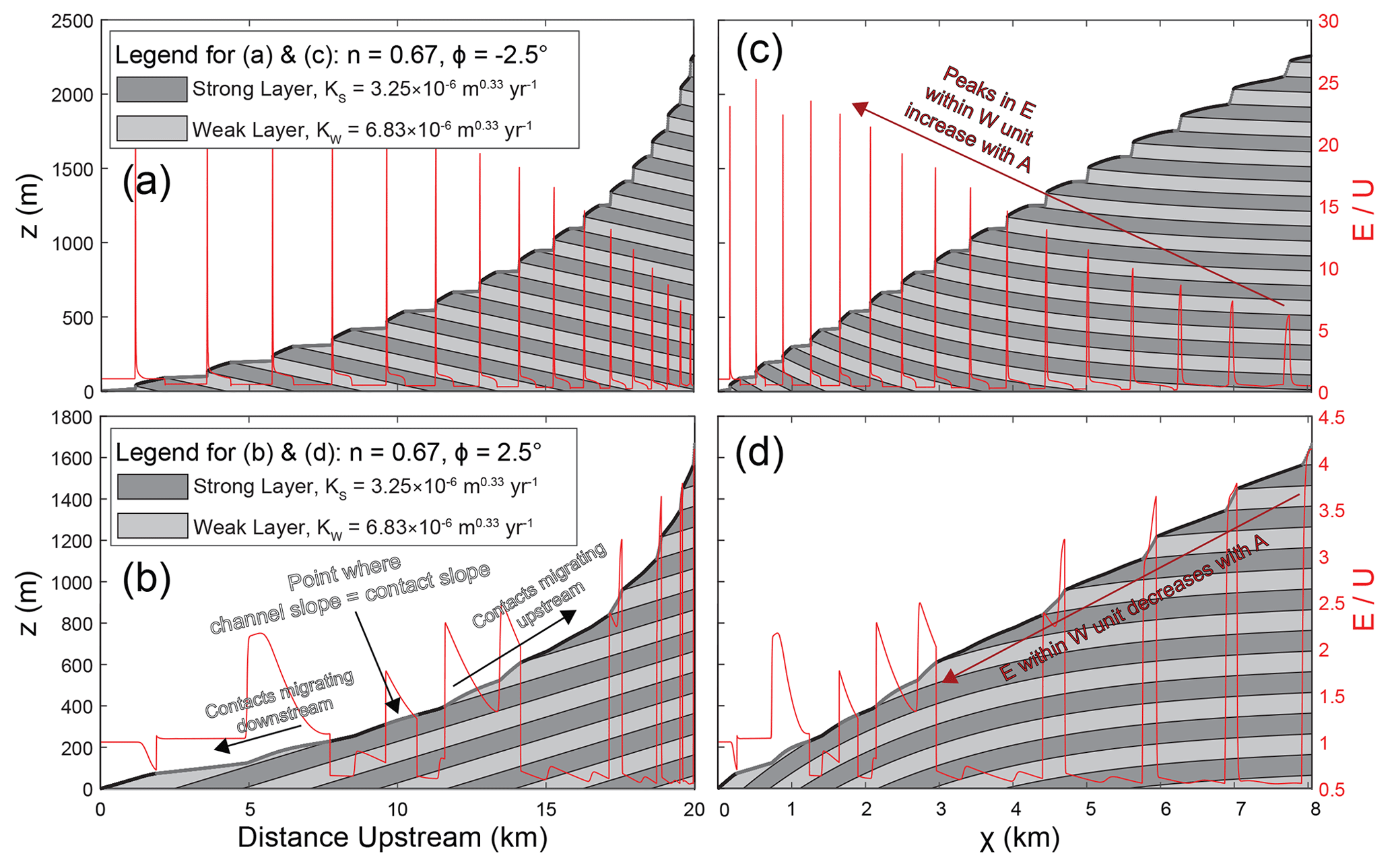
Figure 7Longitudinal profiles (a, b) and χ plots (c, d) for two different simulations with n=0.67. The simulation in (a) and (c) has contact dip ∘, while the simulation in (b) and (d) has ϕ=2.5∘. Layer thickness H and rock-uplift rate U are 100 m and 0.15 mm yr−1 in both simulations, respectively.
The two simulations in Fig. 8 have n=1.5 and the same erodibility (K) values used in Fig. 3b, but with nonzero contact dips. Because we examined simulations with the same absolute contact dips in Fig. 7 (∘), we now show simulations with dissimilar contact dips: Fig. 8a and c have contacts dipping 10∘ upstream (∘), while the simulation in Fig. 8b and d has contacts dipping 1∘ downstream (ϕ=1∘). These two simulations with n=1.5 (Fig. 8) also have distinct morphologies relative to similar simulations with a contact dip of 0∘ (Fig. 3b). For example, the maximum elevations for Figs. 3b, 8a, and 8b are about 2200, 2600, and 2000 m, respectively, even though the erodibilities used are the same. These distinctions highlight the role of contact dip in bedrock river morphology. Even a contact dip of 1∘ causes a striking departure from the behaviors expected for horizontal bedding (Fig. 8b and d). For example, even though the simulation in Fig. 8b is the same as that in Fig. 3b except for a contact dip of 1∘, these two simulations have very different spatial patterns in erosion and steepness (i.e., peaks in erosion rate that increase moving downstream in Fig. 8b vs. a more consistent covariation of erosion rate with rock type in Fig. 3b). With n>1 and contacts dipping 1∘ in the downstream direction (Fig. 8b), erosion rates are no longer relatively uniform within each rock type. Instead, there are sharp peaks in erosion rate near contacts (i.e., consuming knickpoints), and these peaks increase in magnitude with distance downstream.
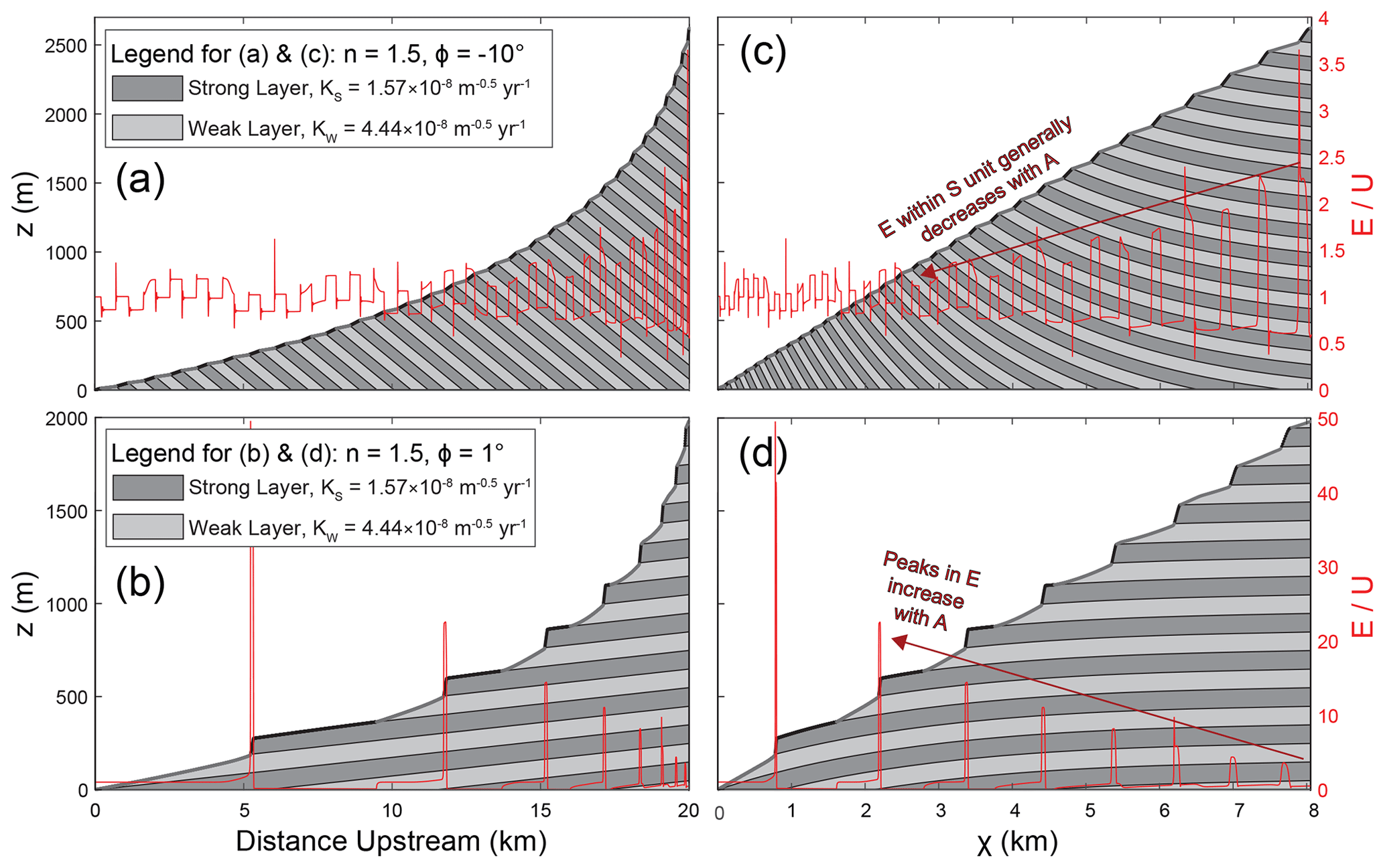
Figure 8Longitudinal profiles (a, b) and χ plots (c, d) for two different simulations with n=1.5. The simulation in (a) and (c) has contact dip ∘, while the simulation in (b) and (d) has ϕ=1∘. Layer thickness H and rock-uplift rate U are 100 m and 0.15 mm yr−1 in both simulations, respectively.
Figures S12–S16 demonstrate that influences the rates at which erosion rates vary with drainage area when contact dips are nonzero. For example, the peaks in erosion rate that increase with drainage area in Fig. 8c would (1) have a smaller range and increase at a slower rate if was lower and (2) have a larger range and increase at a faster rate if m/n was higher.
3.3.2 Contact migration rates for nonzero contact dips
We now examine the contact migration rates in simulations with nonzero contact dips (scenarios 3 and 4; Table 1). Scenario 3 has contacts dipping in the upstream direction (ϕ<0∘), while scenario 4 has contacts dipping in the downstream direction (ϕ>0∘). In this section, we utilize these simulations' contact migration rates to explain the bedrock river dynamics discussed in Sect. 3.3.1 above (i.e., why erosion rates change along the profile).
Figure 9 shows contact migration rate (ddt) versus drainage area for each of the four simulations in Figs. 7 and 8. Like in Fig. 4, the measured contact migration rates in Fig. 9 are gray circles with black outlines, and vertical bars represent the standard deviation of ddt within each drainage area bin. The red dashed line, red symbols, and blue symbols are the kinematic wave speed estimates made with Eqs. (12) and (13); we will address these estimates after exploring general trends in the measured ddt data. The simulations in Fig. 9a and c have contacts dipping in the upstream direction (Fig. 7a and b), while the simulations in Fig. 9c and d have contacts dipping in the downstream direction (Fig. 8a and b). Unlike simulations with a flat-lying stratigraphy, these simulations with nonzero contact dips have contact migration rates that do not follow a consistent power-law relationship with drainage area. Because our results in Sect. 3.1 established that contact migration rates are a reflection of kinematic wave speeds, these results show that for nonzero contact dips, the rate at which kinematic wave speed (CH) increases with drainage area is a function of contact dip. These results confirm the implications of Eq. (12) (Darling et al., 2020); contacts dipping in the upstream direction (Fig. 9a and c) decrease the rate at which kinematic wave speed increases with drainage area, and contacts dipping in the downstream direction (Fig. 9b and d) increase the rate at which kinematic wave speed increases with drainage area.
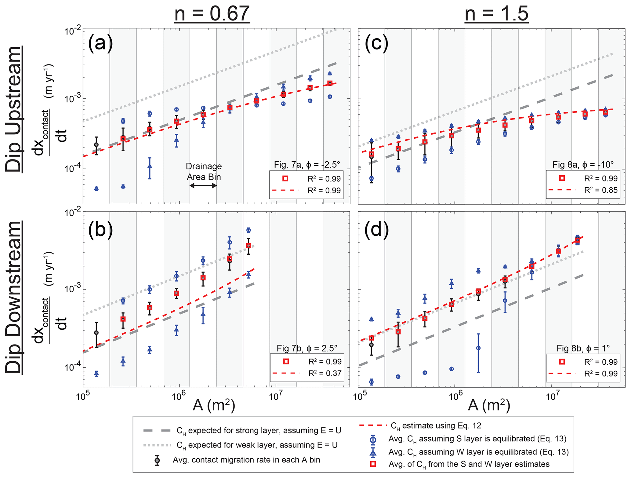
Figure 9Contact migration rates (ddt) vs. drainage area (A) for the four simulations shown in Figs. 7 and 8. The simulations have slope exponent (n), weak erodibility (KW), and strong erodibility values (KS) of (a, b) n=0.67, m0.33 yr−1, and m0.33 yr−1 and (c, d) n=1.5, m−0.5 yr−1, and m−0.5 yr−1.
We now discuss the drivers of these relationships. Even when contact dip is nonzero, a stream can adjust to maintain equal retreat rates on either side of a contact in the same manner discussed in Sect. 3.1 (i.e., an effective adjustment within the strong layer when n>1 vs. resistance in the strong layer when n<1). When contact dip is nonzero, however, the important distinction is that the contact's geometry relative to the channel can limit or enhance the contact's migration in the upstream direction. The migration rates of contacts that dip in the downstream direction (ϕ>0∘) will be enhanced because the erosion of the contact will cause the contact to be exposed further upstream. Conversely, the migration rates of contacts that dip in the upstream direction (ϕ<0∘) will be limited because the contact plane recedes deeper into the subsurface in the upstream direction. The magnitudes of these influences depend on the contrast between channel slope and contact slope, and this contrast changes with drainage area.
Now, we explain these dynamics by examining the relationship between kinematic wave speed and erosion rate when contact dips are nonzero. Even when contact dip is nonzero, slope exponent n controls the relationship between a stream's kinematic wave speed (CH) and erosion rate (E; Eq. 6). We will first discuss cases with n<1. When n<1, then CH is inversely proportional to E (Eq. 6). If contacts are dipping upstream (ϕ<0∘) so that the growth rate of CH with drainage area must gradually decrease (e.g., Fig. 9a), then a stream with n<1 will achieve this decreased growth in CH by having large spikes in channel slope and erosion rate near the contacts (Fig. 7c). The magnitudes of the erosion rate spikes increase with drainage area because the growth rate of CH will decrease with drainage area (to maintain equal retreat rates on either side of a contact). These spikes in erosion will also occur in the weak unit near the contact, as the weaker unit's larger erodibility requires a greater reduction in kinematic wave speed. Conversely, if contacts are dipping downstream (ϕ>0∘) then the growth rate of CH with drainage area will increase (e.g., Fig. 9b). A stream with n<1 will achieve this acceleration in the growth of CH with drainage area through a reduction in the weak unit's erosion rate with drainage area (Fig. 7d). We have highlighted such erosion rate variations in Fig. 7.
If slope exponent n>1, the same trends in kinematic wave speed will occur across the profile (i.e., changing growth rate with drainage area). Importantly, however, the same CH requirements will be met with erosion rate variations that are the opposite of those occurring when n<1. This distinction lies in the fact that when n>1, CH is proportional to E (Eq. 6). For example, if contacts dip upstream (ϕ<0∘) and n>1 then a decrease in the growth rate of CH with drainage area (Fig. 9c) is achieved through a decrease in erosion rate with drainage area (Fig. 8c). If contacts instead dip in the downstream direction (ϕ>0∘) and n>1, then an increase in the growth rate of CH with drainage area (Fig. 9d) is achieved through an increase in erosion rates near contacts (Fig. 8d; the undercutting of the strong unit by the weak unit creates a consuming knickpoint, and the positive contact dip allows the knickpoint to migrate farther upstream). We have highlighted such erosion rate variations in Fig. 8. These spatial variations in erosion rate occur so the stream maintains equal retreat rates on either side of each contact. When contact dips are nonzero, the magnitude of contact slope relative to channel slope changes as a function of drainage area. This relationship causes the influence of contact migration on channel slope to change with drainage area.
Overall, the spatial patterns in kinematic wave speed (increasing or decreasing growth rate with drainage area) depend on contact dip and are independent of slope exponent n, but n controls the spatial patterns in erosion rate that accomplish the required patterns in kinematic wave speed. Although contact migration rates continue to reflect the pattern of kinematic wave speeds across the profile when dip is nonzero, the erosion rates that are representative of these kinematic wave speeds can be highly localized near the contacts (e.g., consuming knickpoints in Fig. 8d).
3.3.3 Kinematic wave speeds for nonzero contact dips
In this section, we test both (1) the framework for kinematic wave speed (CH) developed by Darling et al. (2020) for bedrock river incision through nonhorizontal strata (Eq. 12) and (2) our approach for estimating kinematic wave speed with channel steepness values (Eq. 13). We test these approaches by comparing contact migration rates measured in our models with CH estimates made with Eqs. (12) and (13) for all simulations in scenarios 3 and 4 (Table 1).
The red dashed lines in Fig. 9 are CH estimates made with Eq. (12). These curves capture how the growth rate of kinematic wave speed with drainage area must accelerate or decelerate for positive and negative contact dips, respectively. While capturing the overall trends, the approach of Darling et al. (2020) (Eq. 12) does deviate in some situations. For example, the R2 values for these estimates (relative to the average contact migration rates in each drainage area bin) are high for upstream-dipping contacts and n<1 (R2=0.99; Fig. 9a) but relatively low for downstream-dipping contacts and n<1 (R2=0.37; Fig. 9b). Such deviations occur because Eq. (12) was derived on the assumption that the less steep layer has erosion rates equal to the rock-uplift rate. This assumption is why, for example, the red dashed line starts out along the dark gray dashed line at low drainage areas in Fig. 9b. Like in Fig. 4, this gray dashed line represents the kinematic wave speeds expected for the strong layer if its erosion rate was equal to the rock-uplift rate. In this simulation, however, the strong layer's erosion rates at low drainage areas are lower than the rock-uplift rate (Fig. 7d). This deviation from the assumptions made by Darling et al. (2020) causes the modeled contact migration rates to be higher than the red dashed line (Fig. 9b).
Now, we present examples of estimating kinematic wave speed (CH) with our approach (Eq. 13). In Fig. 9, the blue circles are the average Eq. (13) estimates made with the strong layer's ksn, while the blue triangles are the average Eq. (13) estimates made with the weak layer's ksn. Vertical bars on each value represent the standard deviation of Eq. (13) estimates within each drainage area bin (due to variations in ksn; these examples use the entire 10 Myr of recorded ksn rather than only the final time step). When n<1 (Fig. 9a and b), the CH estimates made with the strong layer are higher than measured contact migration rates. Conversely, when n>1 (Fig. 9c and d) the CH estimates made with the weak layer are higher than measured contact migration rates. These estimates are too high because the corresponding layer tends to have an erosion rate E that is lower than the rock-uplift rate U (strong layer when n<1, weak layer when n>1). The other layer's erosion rate will be higher than U, however, and taking the average of Eq. (13) estimates made for the strong and weak layers produces an extremely accurate depiction of the measured contact migration rates. For example, the red squares in Fig. 9 are the average of the weak and strong layers' Eq. (13) estimates of kinematic wave speed. Relative to the measured contact migration rates, these red squares have R2 values of 0.99 in each panel in Fig. 9. Note that there is no Eq. (13) estimate in the lowest drainage area bin of Fig. 9b because, in this case (n<1), reaches in the weak layer tend to be less steep. Because the reaches in the weak unit are less steep, they span a longer horizontal distance along the channel. As a result, an entire reach within the weak unit would not fit within the lowest drainage area bin in this simulation.
To test the influence of binning results by drainage area, we created a version of Fig. 9 with 20 drainage area bins instead of 10 (Fig. S12). The relationships between measured contact migration rates and estimated kinematic wave speeds are generally the same. For example, the R2 values for Eq. (12) and (13) estimates of CH in each panel in Fig. S12 are the same as those in Fig. 9 with only one exception (the Eq. 12 estimate in panel b has an R2 value of 0.41 instead of 0.37). We binned results by drainage area for visual clarity in our figures, but these results show that the approach does have a slight impact on our results.
To test the accuracies of Eqs. (12) and (13), Fig. 10 shows estimates of kinematic wave speed (CH) made with Eqs. (12) and (13) relative to contact migration rates (ddt) measured in all simulations with nonzero contact dips (scenarios 3 and 4; Table 1). In each panel, the estimated kinematic wave speeds closely follow a 1:1 relationship with measured contact migration rates. These findings demonstrate that contact migration rates reflect kinematic wave speeds even for nonzero contact dips, just as demonstrated for horizontal contacts in Fig. 5. Figure 10 therefore highlights the fact that both contact migration and its consequences for bedrock rivers (e.g., variations in channel steepness and erosion rate) are predictable phenomena. Note that these Eq. (13) estimates only use the ksn recorded in one model time step rather than the entire 10 Myr of recorded values. This choice was motivated by the data limitations for real streams. Figure S18 shows Eq. (13) estimates using all recorded ksn; the accuracy is similarly high, except there are more data points.
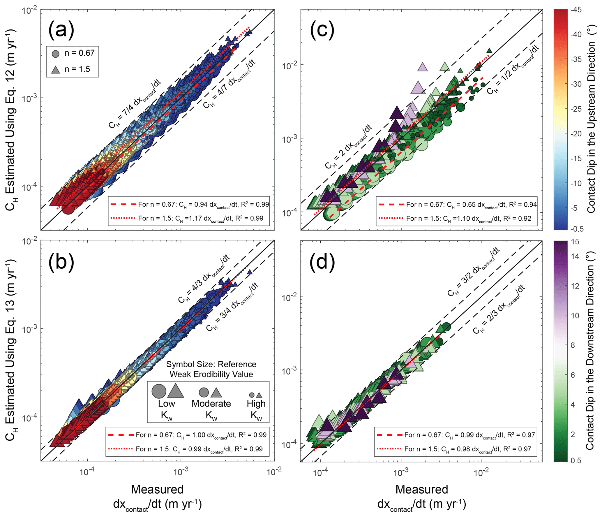
Figure 10Contact migration rates measured in our models (ddt) vs. kinematic wave speeds (CH) estimated using Eqs. (12) and (13). Each point represents one drainage area bin in one simulation. Panels (a, b) show results for scenario 3 (contacts dipping upstream, ϕ<0∘), and panels (c, d) show results for scenario 4 (contacts dipping downstream, ϕ>0∘). Dashed lines show the minimum and maximum values for most values in each panel, with labels denoting the corresponding relationships between contact migration rate and kinematic wave speed.
The contact migration rates and kinematic wave speeds for the six additional simulations using ∘ and values of 0.3, 0.5, or 0.7 are presented in Figs. S14–S16. The CH values estimated with Eqs. (12) and (13) are still accurate portrayals of modeled contact migration rates even for simulations using different values.
Overall, both Eqs. (12) and (13) provide highly accurate portrayals of the contact migration rates in our numerical models (Figs. 10 and S14–S16). Even though Eq. (12) can be less accurate at times (Fig. 9), the equation's performance is consistently good across the parameter space explored in scenarios 3 and 4 (Fig. 10). We show how Eqs. (12) and (13) can be combined to estimate erodibility in Sect. 3.3.5, but we will first more thoroughly explore how erosion rates vary for nonzero contact dips (Sect. 3.3.4).
3.3.4 Erosion rate variations for nonzero contact dips
In this section, we explore the variations in erosion rate that occur for nonzero contact dips in greater detail. Through these analyses, we develop three-dimensional regressions between K*, , and (Eq. 11). Recall that ϕχ is the contact dip in χ space (nondimensional; change in contact elevation change in the overlying river's χ values) and K* is a term describing erodibility contrasts (Eq. 7c). The purpose of this analysis is to (1) highlight the magnitude of erosion variations that occur when contact dip is nonzero and (2) relate these variations to both drainage area and contact dip.
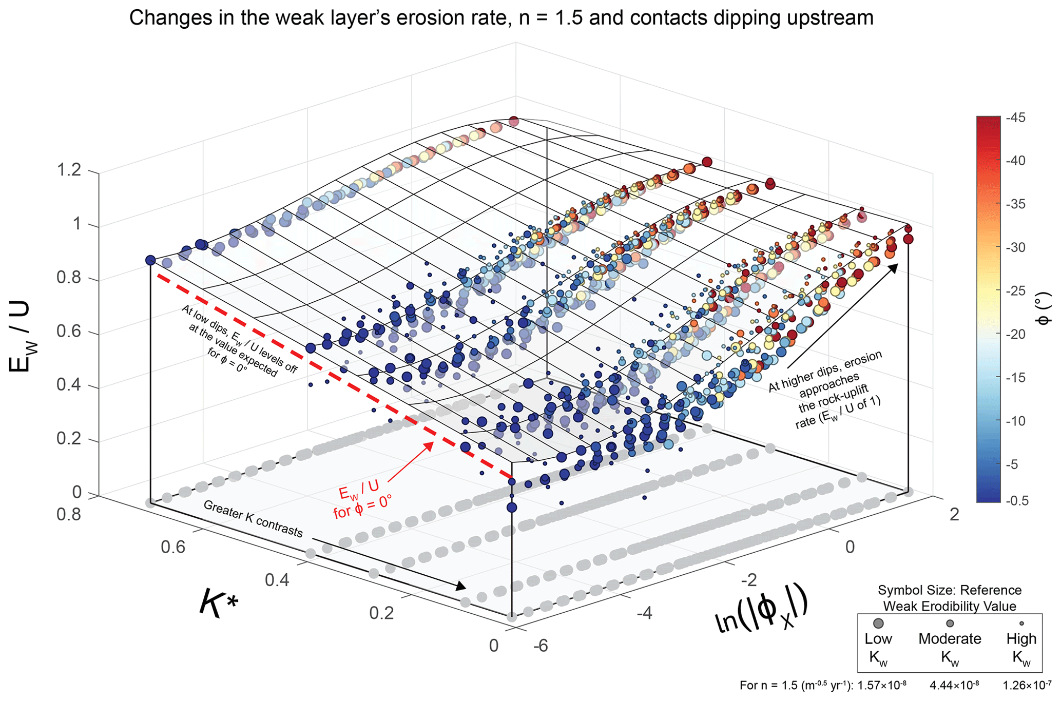
Figure 11Variations in the average erosion rate in the weak layer (EW) normalized by rock-uplift rate (U) with both the logarithm of the absolute contact dip in χ space () and the enforced K* (Eq. 7c) for simulations with n=1.5 and contacts dipping upstream (ϕ<0∘). A regression is fit to all data (R2=0.81): . The reasons why there are no small symbols for the highest K* are discussed in Sect. S3 (i.e., the damping length scales were too large in those simulations; Perne et al., 2017).
Figure 11 shows the erosion rates in the weak layer (EW) normalized by rock-uplift rates (U) for all simulations with n=1.5 and contacts dipping upstream (ϕ<0∘; scenario 3). There are gray shadows on the –K* plane situated directly beneath each point. Each and value is the average within one drainage area bin (e.g., Fig. 9) in one simulation. Across the parameter space used for the simulations in Fig. 11, there is a consistent trend in . At large erodibility contrasts (for n>1, low K*), the weak layer erodes at a rate much lower than the rock-uplift rate. At small erodibility contrasts (for n>1, high K*), the variations in erosion rate are more subdued. The magnitude of also influences erosion rate. For example, when is high all values approach 1. At low values, the erosion rates approach those expected for a contact dip of 0∘ (dashed red line; Eq. 10). Note that increases with distance downstream along a profile (i.e., at higher drainage areas, the channel slope is smaller relative to contact slope). Because of this relationship, represents a combination of (1) position along the stream profile and (2) the magnitude of contact dip. Higher contact dips and/or larger drainage areas increase , causing to approach values of 1. Lower contact dips and/or smaller drainage areas decrease , causing to approach the values expected for a contact dip of 0∘ (red dashed line). The multilinear regression shown in Fig. 11 (R2=0.81) captures these relationships between erosion rate (), erodibility contrasts (K*), and both drainage area and contact dip (). The residuals for this regression are shown in Fig. S19.
We present Fig. 11 to demonstrate general trends in erosion rate for nonzero contact dips, but we provide similar figures for other combinations of unit type (i.e., strong or weak), slope exponent n, and contact dip in Figs. S20–S30. We always fit multilinear regression between K*, , and the weak layer's normalized erosion rate (), but we also fit a multilinear regression for the strong unit () when n=0.67 and contacts dip downstream (ϕ>0∘). Otherwise, the erosion rates within the strong unit are not captured well by such regressions (e.g., greater deviations from the overall trend). The other regressions we evaluate vary in their accuracy, with R2 values ranging from 0.32 (Fig. S22) to 0.92 (Fig. S24). Like the regression in Fig. 11, however, these regressions always highlight the roles of K* and in setting the magnitudes of erosion rate variations. K* reflects what the erosion rates would be if the contact dip was 0∘ (e.g., red dashed line in Fig. 11), while variations in ) values control how different portions of the profile approach the erosion rates expected for 0∘ (reflecting the combined influence of drainage area and contact dip).
There is an important distinction to note regarding one of the other regressions, however. When contacts dip downstream (ϕ>0∘) and n=1.5, there is a change in how erosion rates vary with (Fig. S22). Because the growth rate of kinematic wave speed increases with drainage area when ϕ>0∘ (e.g., Fig. 9d), consuming knickpoints naturally form when n>1 (e.g., Fig. 8b). These consuming knickpoints cause erosion rates to dramatically increase with (e.g., EW>10 U at high and high erodibility contrasts). This dramatic increase in erosion rate with only occurs for those conditions (n>1 and ϕ>0∘) due to the formation of consuming knickpoints.
To summarize the results for this section, when contact dips are nonzero the erosion rates within each unit change as a function of contact dip, drainage area (which both set ϕχ), and erodibility contrasts (K*). Assuming that the erosion rate is equal to the base-level fall rate (Eq. 12) will cause one to overestimate kinematic wave speed (CH) when n>1 (e.g., Fig. 9c) and underestimate CH when n<1 (e.g., Fig. 9b). Note that our intention is not to assign theoretical significance to these three-dimensional regressions, but only to use them to highlight how contact dip, drainage area, and erodibility contrasts influence the erosion rates for nonzero contact dips.
3.3.5 Estimating erodibility in our numerical models using nonzero contact dips
In this section, we evaluate how accurately the erodibility (K) in our numerical models can be estimated using channel steepness (ksn) without a priori information on erodibility. We demonstrated that Eqs. (12) and (13) are generally accurate within numerical models (Fig. 10), but now we demonstrate how the two equations can be combined to estimate erodibility. The purpose of this analysis is to provide context for our analysis of Tank Wash near Hanksville, UT (Sect. 3.4). We will attempt to quantify erodibility using the channel steepness observed along Tank Wash, so our intention here is to test how accurately one can estimate erodibility in numerical models for which the true erodibility values are known.
Figures 12 and 13 summarize how the K values we use in our numerical models can be estimated by combining Eqs. (12) and (13). Figure 12 focuses on weak erodibilities (KW) used in our numerical models, while Fig. 13 focuses on the strong erodibilities (KS). Figures 12a–b and 13a–b show the X2 values calculated between (1) the CH estimates made with Eq. (12) for a range of erodibilities and (2) the CH estimates made with Eq. (13) for the ksn recorded in each simulation's final time step. We chose to use only one time step of recorded ksn values due to the data limitations for real rivers, but Figs. S31 and S32 are versions of Figs. 12 and 13 that use all ksn recorded over the 10 Myr for each simulation. The x axes of Figs. 12a–b and 13a–b represent the entire range of K values assessed normalized by the actual weak or strong erodibility used in that simulation (KW in Fig. 12, KS in Fig. 13). Each line represents one simulation (blue for simulations with ϕ<0∘, red for simulations with ϕ>0∘). Each of these lines has a minimum X2 value, and invariably this minimum occurs near an assessed K enforced K value of 1.

Figure 12Comparison of best-fit K values in our numerical models to the weak erodibility (KW) used in each simulation. (a, b) X2 misfit function values for kinematic wave speeds (CH) estimated using Eq. (12), the enforced contact dip (ϕ), and a wide range of K values (200 points spaced logarithmically from 10−9 to 10−4 m1−2nθ yr−1, where θ=0.5) relative to the Eq. (13) estimates of CH. (c, d) Comparison between the best-fit K and the KW enforced in the simulations. Panels (a) and (c) show results for n=0.67, while panels (b) and (d) show results for n=1.5.
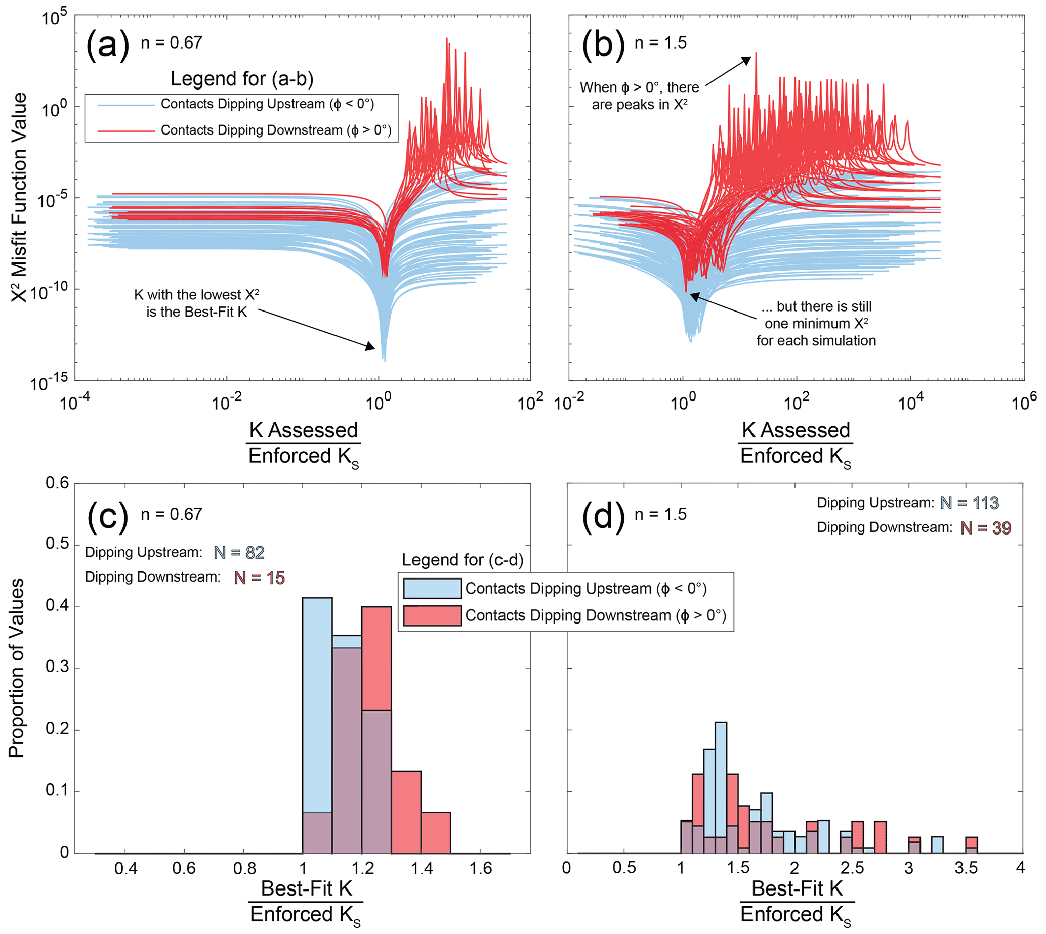
Figure 13Comparison of best-fit K values in our numerical models to the strong erodibility (KS) used in each simulation. (a, b) X2 misfit function values for kinematic wave speeds (CH) estimated using Eq. (12), the enforced contact dip (ϕ), and a wide range of K values (200 points spaced logarithmically from 10−9 to 10−4 m1−2nθ yr−1, where θ=0.5) relative to the Eq. (13) estimates of CH. (c, d) Comparison between the best-fit K and the KS enforced in the simulations. Panels (a) and (c) show results for n=0.67, while panels (b) and (d) show results for n=1.5.
Figures 12c–d and 13c–d are histograms showing the distributions of the best-fit K (those with the minimum X2 values) relative to the actual weak and strong erodibilities (KW in Fig. 12, KS in Fig. 13). The x axes for these histograms (best-fit K enforced K) use bin sizes of 0.1. The best-fit K is almost always between KW and KS (there are some exceptions with (best-fit ) > 1 in Fig. 12d). The best-fit K can be much larger than KS when n>1 (Fig. 13d) because the strong layer tends to have larger deviations in erosion rate relative to the rock-uplift rate under those conditions (Figs. S26 and S28). Conversely, the rock type that tends to have lower steepness (weak layer when n>1, strong layer when n<1) tends to have smaller deviations in erosion rate relative to the steep layer (Figs. 11 and S19–S30). As a result, the best-fit K values in Figs. 12 and 13 are more consistently close to the K for the layer that tends to have lower steepness. These results suggest that an erodibility estimated using this approach is more likely to be representative of the rock type with lower steepness (weak layer when n>1, strong layer when n<1). Figures 12 and 13 highlight the potential to estimate erodibility using observed channel steepness (ksn), known contact dips (ϕ), and a known base-level fall rate (U).
3.4 Analysis of Tank Wash
In this section, we apply the methods developed in this study (Sect. 3.3.5) to Tank Wash (Fig. 14). Figure 14a shows inferred contacts labeled with purple lines. The units clearly dip to the west–southwest here, which is generally in the upstream direction for Tank Wash. Using the (1) potential contacts identified using Google Earth and a nearby geologic map (Doelling et al., 2015) as well as (2) changes in steepness along Tank Wash, we then estimated the contact locations along the stream's longitudinal profile (Fig. 14b). Tank Wash flows across a wide range of lithologies, including sandstone, mudstone, shale, and siltstone, and these units likely offer different levels of resistance to fluvial erosion. In Fig. 14b, these contacts are projected into the subsurface using an assumed contact dip (ϕ) of −1∘ (note the vertical exaggeration). Each of the potential contacts we identified occur at a change in channel steepness; there are three locations where steepness changes, but we could not confidently infer a change in lithology. We highlight those three locations in Fig. 14a and b. Those steepness changes could indicate, for example, changes in rock strength within one unit. It is important to note, however, that our models suggest that changes in steepness can occur both at contacts and some distance away from contacts (e.g., Figs. 7a and 8b).

Figure 14Overview of Tank Wash, a stream near Hanksville, UT. Panel (a) is a Google Earth image (© Google Earth) with the stream and geology shown. Panel (b) is a longitudinal profile for Tank Wash with the assumed contacts from (a) shown as gray lines. The average steepness (ksn) for each reach situated between these contacts is shown in red. The lithologies are as follows: Kmf is brown sandstone and mudstone; Kmt is gray shale, siltstone, and mudstone; Kcmu and Jmb are color-banded siltstone, claystone, mudstone, and shale; Jms contains both red–brown mudstone and siltstone as well as light-yellow–gray lenticular sandstone and conglomerate; and Js is red–brown siltstone, sandstone, and gypsum.
Figure 15a is a slope–area plot, with the inferred contact locations shown as vertical dashed lines and the average steepness values of the reaches between each contact shown as dotted lines. We used these average steepness values to estimate kinematic wave speeds (CH) using Eq. (13) (Fig. 15b and c). For the two U values assessed (0.3 and 0.85 mm yr−1), the patterns in the data are the same but CH magnitudes are scaled by the assumed U. We estimated two kinematic wave speeds for each stream reach defined by the inferred contacts: one CH at the lowest drainage area of the reach and one at the highest. In Fig. 15b and c, each pair of CH estimates is connected by a dashed line. If Tank Wash has achieved a dynamic equilibrium (i.e., variations in steepness and erosion rate are due to contact migration rather than changes in base-level fall), our results have shown that the true CH values should lie between the highest and lowest estimates (Eq. 13). To pursue this balance, we therefore evaluated the average CH within five bins spaced logarithmically from the lowest to the highest drainage areas. These average CH values are shown in Fig. 15b and c as black squares with horizontal bars extending across the corresponding drainage area bin. Although this approach is not the same as taking the average of Eq. (13) estimates made separately for weak and strong units (e.g., Fig. 9), our intention is only to pursue moderate values situated between the highest and lowest CH estimates in Fig. 15b and c.
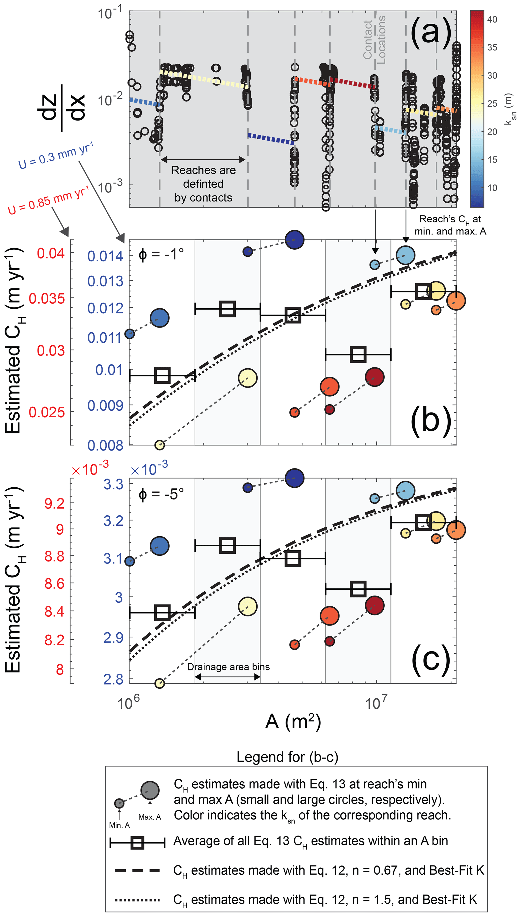
Figure 15Preliminary analysis for Tank Wash. (a) Slope–area plot with gray dashed lines for each presumptive contact identified in Fig. 14. The average steepness (ksn) of each reach between contacts is shown as colored dotted lines. (b, c) Kinematic wave speed values (CH) estimated with Eq. (13) using the average ksn values, rock-uplift rate U=0.3 mm yr−1 or U=0.85 mm yr−1 (separate axes), and contact dip (ϕ) values of either (b) −1∘ or (c) −5∘. See Fig. 16 for the best-fit K values.
The dashed and dotted black lines in Fig. 15b and c are the Eq. (12) kinematic wave speeds for the best-fit erodibility values. These best-fit K values are those with the lowest X2 misfit function value (Eq. 14) relative to the average Eq. (13) estimates of CH (black squares in Fig. 15b and c). The X2 values for all K are shown in Fig. 16. The K values range from 10−8 to 10−2 m1−2nθ yr−1 (where θ=0.5), and for each combination of contact dip, base-level fall rate, and n, there is one K corresponding to the minimum X2. Varying the contact dip does not change the selection of a best-fit K because contact dip scales both the Eqs. (12) and (13) estimates (Fig. 14b and c). Varying either base-level fall rate or slope exponent n does, however, alter best-fit K values (Fig. 16). Although the two different base-level fall rates (U) produce distinct best-fit K values, the best-fit K values for each n differ by a factor of ∼2.83 because the two U values used differ by a factor of ∼2.83. If we used U=0.15 mm yr−1 instead of 0.3 mm yr1, for example, we would obtain a best-fit K value that was half of that for U=0.3 mm yr−1. This finding indicates that accurately constraining U is important. The uncertainty involved in erodibility can be orders of magnitude (Stock and Montgomery, 1999), however, so being able to gain some quantitative constraints on K for a reasonable range of erosion rates is certainly an advancement. Based on results from our numerical models (Figs. 12 and 13), we would argue that these erodibilities are (1) likely between the highest and lowest erodibilities present and are (2) likely more representative of the unit with the lowest steepness. Because Tank Wash has its lowest steepness values in areas we infer to have mudstone and/or siltstone (Kmf, Kmcu, and Jms; Fig. 14), it is possible that these erodibilities are more representative of those units. Because one may intuitively expect mudstone and siltstone to be weaker than other units present, like sandstone, then the lower steepness within those seemingly weaker units could suggest a slope exponent n that is greater than 1. Although there are considerable uncertainties involved in this inference, Darling et al. (2020) also found that streams incising through sedimentary units in southern Utah had morphologies that were consistent with n>1.
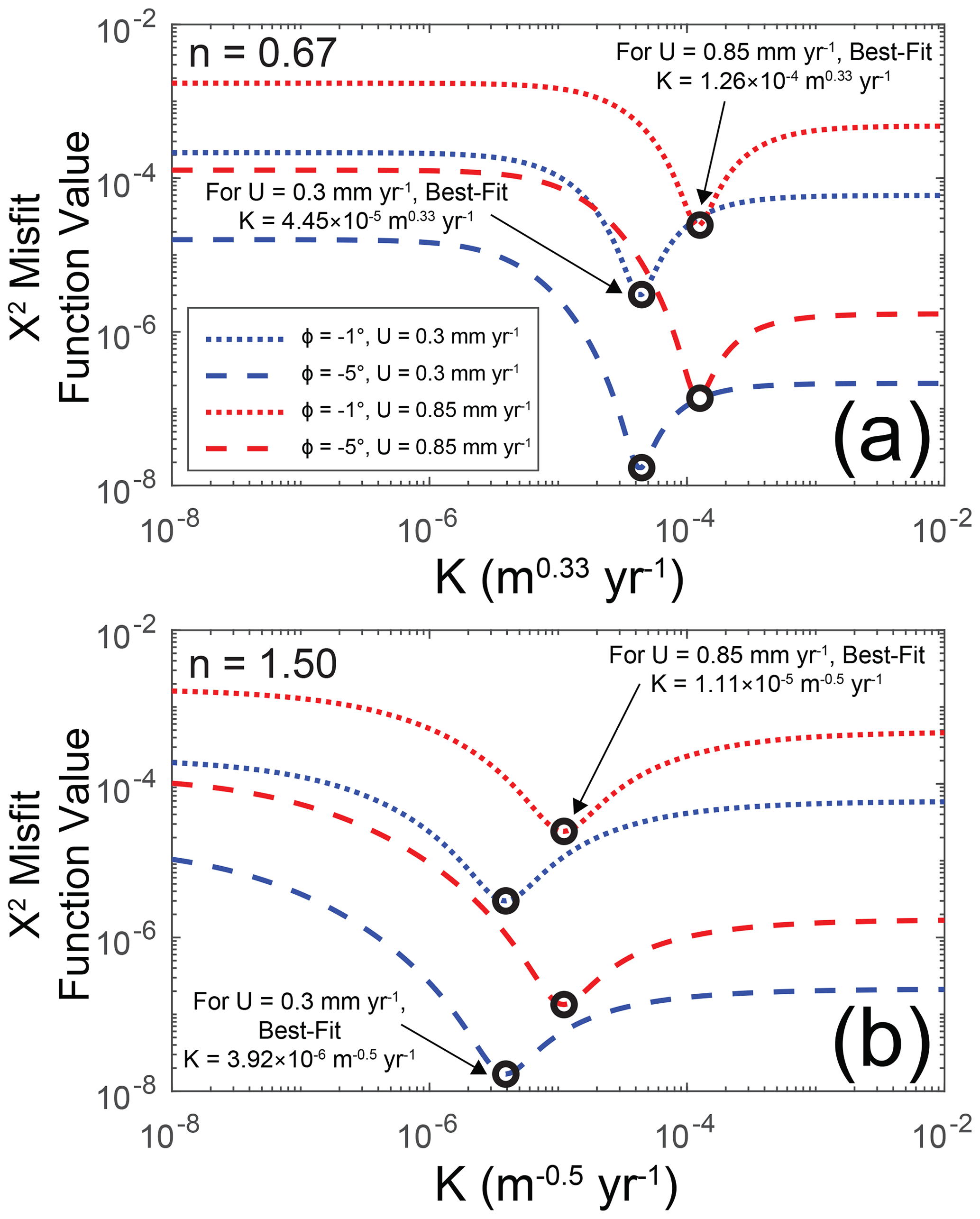
Figure 16X2 misfit function values for kinematic wave speed (CH) estimates made with Eq. (12) and a wide range of erodibility (K) values relative to the CH estimated for Tank Wash with Eq. (13) (Fig. 15). Panel (a) shows results for n=0.67, while panel (b) shows results for n=1.5. Also note that the X2 values are lower for ∘ because a greater dip in the upstream direction causes a smaller range of kinematic wave speeds (e.g., Fig. 9c). The misfit for this reduced range can be smaller, but these lower X2 values do not indicate that the dip is closer to −5∘ than to −1∘.
We have shown here that for rivers incising into layered rocks, channel steepness, erosion rates, and contact migration rates continue to reflect rock strength differences across a wide range of contact dips. Changes in river erosion and morphology with dip are predictable, enabling the perturbation of contact migration to be exploited for insight rather than avoided or ignored. This finding also emphasizes that the effects of mixed lithologies must always be weighed when considering (1) bedrock river morphology and (2) erosion rate estimates based on techniques like detrital cosmogenic nuclide analysis (Darling et al., 2020).
4.1 Evaluation of previous work
Our findings demonstrate that when contacts are horizontal (ϕ=0∘), the equations developed by Perne et al. (2017) (Eqs. 7c and 10) remain applicable even if there are large changes in parameters like erodibility, rock-uplift rates, and layer thicknesses. We have also shown here that when there are more than two rock types, contact dips of zero, and the stream has achieved a dynamic equilibrium, stream reaches in each rock type will erode at rates that provide a uniform trend in kinematic wave speed (CH) across the profile. Whether a unit erodes above or below rock-uplift rate U depends on the slope exponent n value and the magnitude of the layer's erodibility in relation to the other layers' erodibilities. We have also shown that the erosion rates expected for a contact dip of 0∘ are important when contact dips are nonzero; portions of the profile with high channel slope (relative to the absolute value of contact slope) can approach these erosion rates even when contact dip is nonzero (i.e., low values in Fig. 11).
Our results also demonstrate that the equation for kinematic wave speed (Eq. 12) developed by Darling et al. (2020) is a robust depiction of contact migration rates for nonzero contact dips (Fig. 10). Although this approach can be less accurate at times (Fig. 9), the magnitudes of such deviations are small in relation to the potential variations in erodibility. As a result, we were able to use their approach to accurately estimate the erodibilities used in our numerical models (Figs. 12 and 13). These authors also developed an expression for the erosion rate required for reaches in a strong unit to have the same kinematic wave speed as the weak unit (which was assumed to erode at the base-level fall rate). Although we focus on how erosion rates in the weak unit can deviate from the base-level fall rate (Fig. 11), the expression developed by Darling et al. (2020) could be applied with modified erosion rates in the weak unit.
4.2 Influence of rock strength contrasts on the pursuit of equilibrium
Because our results demonstrate the complexity of patterns in channel steepness and erosion rate along rivers eroding through layered rocks, these complexities must be considered within the adjustment of landscapes. If contact migration perturbs channel slopes and erosion rates in real landscapes, then these perturbations could significantly impact a landscape's adjustment to changes in tectonics or climate. These impacts could shorten or lengthen timescales of transient adjustment. For example, this study and previous work (Darling et al., 2020) have shown that contacts dipping upstream (ϕ<0∘) can cause the growth rate of kinematic wave speed with drainage area to decrease (e.g., Fig. 9a and c). This decrease in the growth of CH with drainage area might increase the response times of a river, perhaps causing the river to effectively have a lower erodibility at higher drainage areas. Conversely, when contacts dip downstream there is an acceleration in the growth rate of CH with drainage area (e.g., Fig. 9b and d). This acceleration in the growth of CH may cause the river to effectively have a higher erodibility at higher drainage areas. As demonstrated by these examples, erodibility could effectively be a function of both rock type and drainage area (), even if the weak and strong erodibilities do not change with drainage area. Otherwise, the combined influence of drainage area and contact dip on erosion rate (Fig. 11) could make higher and lower elevations of a landscape respond differently to changes in climate. For example, erosion rates may deviate farther from base-level fall rates at low drainage areas where channel slope is high relative to the absolute value of contact slope (i.e., low ), and such deviations would cause these drainage areas to respond differently to changes in precipitation. Such dynamics remain to be demonstrated, but the fact remains that geomorphologists' expectations regarding landscape evolution are shaped by the idea that erosion rates will be controlled by base-level fall and climate; our findings and previous work (Forte et al., 2016; Perne et al., 2017; Darling et al., 2020) suggest that rock strength contrasts can also influence erosion rates.
The role of rock strength contrasts in a landscape's adjustment to climate and tectonics is important, but changes in rock strength contrasts may also be capable of driving landscape transience (Forte et al., 2016). We focus here on a stratigraphy with a repeating pattern of rock types, and despite spatial variations in erosion rate the streams eventually achieve a dynamic equilibrium so that the range of elevations is constant with time. The stratigraphic record, however, is far more complicated than the stratigraphy we use. For example, if a stream had equilibrated to incision through two rock types but then a third rock type was exposed, the subsequent changes in erosion rate could begin a long-lasting transience (Forte et al., 2016). Although scenario 2 only uses three rock types instead of two, it was intended to demonstrate that channel slopes in each unit (however many there are) adjust to allow for a consistent trend in CH across the profile. The moderate CH values maintained across the profile, however, depend on the distribution of erodibilities. For example, the exposure of a much stronger unit would lower the profile's CH values, altering the erosion rates in other units and initiating a gradual transient adjustment (potentially lasting until the new unit was uplifted across the profile's fluvial relief). A continuous succession of units with widely varying erodibilities could therefore cause streams to be in a constant state of adjustment, never truly achieving a dynamic equilibrium. Alternatively, landscape transience could be caused by changes in unit thickness, even if the rock types remain the same (i.e., a change towards thicker weak units and thinner strong units would alter fluvial relief). Because we demonstrate that even slight changes in contact dip can cause marked changes in river behavior and morphology (Figs. 3, 7, and 8), one might also imagine that changes in contact dip with time due to tectonic folding could cause temporal changes in the influence of rock strength contrasts (in addition to the base-level changes due to tectonic activity). Furthermore, because we demonstrate that drainage area can influence erosion rates along rivers incising through layered rocks (e.g., values in Fig. 11 are a proxy for drainage area), this consideration could be important for drainage reorganization (Willett et al., 2014). Indeed, the presence of layered rocks can exert a strong influence on drainage network evolution (Ward, 2019; Sheehan and Ward, 2020a, b), and spatial variations in erosion rate due to rock strength contrasts would further complicate both drainage divide migration and stream capture. Because Figs. S12 and S13 demonstrate that influences the variations in both channel slope and erosion rate with drainage area when contact dips are nonzero (potentially influencing spatial contrasts in erosion rate), could be significant for the drainage reorganization of landscapes underlain by layered rocks. To summarize these considerations, the presence of rock strength contrasts might make dynamic equilibrium more of a moving target. With factors like climate and tectonics changing over different timescales, the additional consideration of contrasts in rock strength could make dynamic equilibrium a more elusive consequence for landscape evolution.
4.3 Exploring the role of rock strength contrasts in other models of fluvial erosion
The motivation for this study was to understand the implications of the stream power model for variations in channel slope, erosion rate, and kinematic wave speed for different combinations of contact dip and erodibility contrasts. Before we can test if the common form of the stream power model accurately depicts rivers like those near Hanksville, UT, we must understand the morphological implications of the stream power model. We find here that, according to the common form of the stream power model, variations in channel slope due to rock strength contrasts are set by (1) the rock-uplift rate (U), (2) the contact dip ϕ, (3) the spatial distribution of drainage area, (4) the magnitude of each layer's erodibility (K), as this distribution controls the moderate kinematic wave speeds that the rivers will settle upon (Fig. 4), and (5) the contrast among these erodibilities as represented by K*. The last two points may seem redundant, but the distinction lies in how two river systems may have the same K* value, but the river systems may have erodibilities of differing magnitudes. Overall, our preliminary analysis of Tank Wash suggests that the stream does conform to predictions from the stream power model (e.g., the kinematic wave speeds estimated with Eq. 13 can be approximated using a best-fit erodibility and Eq. 12).
It is important to note, however, that the stream power model (Whipple and Tucker, 1999) depicts shear stress or unit stream power with simplifying assumptions regarding (1) the variations in discharge and channel width with drainage area, (2) the role of sediment cover (Sklar and Dietrich, 2004), (3) the presence of erosion thresholds (DiBiase and Whipple, 2011; Lague, 2014), and (4) the use of a single geomorphically representative flow. Clearly, the stream power model is not fully correct, but that failing does not imply that the model cannot be useful. Gasparini and Brandon (2011) did show, for example, that the saltation–abrasion model (Sklar and Dietrich, 2004), a generalized abrasion model (Parker, 2004), and a transport-limited model could all be expressed in a form consistent with the stream power model. If the results of different portrayals of fluvial erosion can be sufficiently expressed as power-law relationships involving drainage area and channel slope, then our findings may be pertinent to alternative portrayals of fluvial erosion. Clearly, however, there is more work to be done involving the use of other fluvial models. Below, we focus on two considerations we consider to be significant for such modeling efforts: the role of sediment cover and the potential influence of dynamic channel width adjustment.
In this study, we have focused exclusively on detachment-limited rives. Real landscapes will not be purely detachment limited, of course, so the influence of sediment cover on bedrock rivers incising through layered rocks remains an important consideration. For example, Johnson et al. (2009) showed that channel slopes can reflect the characteristics of sediment load rather than bedrock properties. There is likely a threshold in sediment cover over which the dynamics examined here disappear entirely (i.e., the feedbacks between contact migration, channel slope, and erosion rate are hindered by sediment deposition). There could be lower levels of sediment cover, however, where the dynamics we study here still occur albeit at lower magnitudes. Both (1) the extent to which sediment cover must be limited for rock strength contrasts to perturb erosion rates and (2) whether such conditions are likely to occur in real landscapes remain as outstanding questions. Limited sediment cover within all rock types may allow for erosion rate variations, but sediment cover could also covary with rock type. For example, a strong rock type may have limited sediment cover, while a weak rock type has more persistent sediment cover. At present, it is unclear whether these feedbacks can occur if one lithology has transport-limited reaches, while another lithology has detachment-limited reaches. Future work should explore the erosion rate variations within numerical models that can freely transition between detachment-limited and transport-limited fluvial processes (Davy and Lague, 2009; Shobe et al., 2017; Yanites, 2018).
We use the common form of the stream power model here, and this model is constructed with assumptions regarding the scaling between drainage area and channel width (Whipple and Tucker, 1999). If channel width follows an assumed power-law scaling with drainage area, the only aspect of channel morphology that can be adjusted is channel slope. Previous work, however, shows that dynamic channel width adjustment may play a significant role in the transient adjustment of bedrock rivers (Yanites et al., 2010; Yanites, 2018). If the erosion variations caused by rock strength contrasts could be accommodated by variations in channel width or process efficiency (e.g., abrasion vs. plucking; Hancock et al., 1998), then detecting the influence of contact migration in longitudinal profiles could be challenging. Although one might suspect that systematic changes in channel width or erosion processes near contacts should be easily recognizable in the field, the conditions observable in the field may not always be representative of conditions during geomorphically significant flows (e.g, changes in bedrock exposure and erosion processes during floods; Hartshorn et al., 2002). The role of channel width adjustments should be examined in future modeling studies.
4.4 Application of our approach to real landscapes
For our simulations, we focus on rivers incising through a stratigraphy with a spatially uniform contact dip. Real streams can have the apparent dip change over space, however, either through (1) changes in the actual contact dips or (2) changes in the streamflow direction relative to the units' strike. For example, the potential field example shown in Fig. 1 has spatial changes in both contact dip and streamflow directions. Indeed, the stream shown in Fig. 1c has a flow direction that is almost orthogonal to that of Tank Wash (Figs. 1b and 14). We have shown that even slight changes in apparent dip can have a pronounced effect on bedrock river behavior (Figs. 3, 7, and 8), and the different streams near Hanksville may therefore require separate, unique treatments. Although apparent dip could vary along each stream, these streams are generally incising through the same units. Based on the results from our numerical models, such field examples may therefore represent an opportunity to (1) use different streams to sample a wide range of drainage areas and apparent contact dips and (2) search for the erodibilities that would satisfy these disparate river morphologies (i.e., through a combination of Eqs. 12–14). For example, tributary confluences may provide opportunities to corroborate different erodibility estimates for a tributary and the larger river it flows into.
There could certainly be complications in applying our method for estimating kinematic wave speed from steepness (Eq. 13) to real streams. For example, such applications would still require independently constrained base-level fall rates or rock-uplift rates (U), and estimating U can involve a great deal of uncertainty (e.g., cosmogenic erosion rates). Although we are able to accurately estimate CH and K using the steepness within weak and strong units, ksn values along real streams are notoriously variable (Wobus et al., 2006). While our results suggest that one might be able to use variations in channel steepness to gain constraints on slope exponent n (i.e., if n<1 or n>1), the pronounced variations in steepness that can occur in real landscapes would likely impede such an effort.
Although our analysis of Tank Wash suggests that such an approach is promising, we acknowledge that this analysis is far from ideal. A rigorous analysis of Tank Wash requires both detailed field surveys of contact dip and more constraints on the spatial patterns of erosion; has the stream achieved a dynamic equilibrium, or is it in a state of transient adjustment due to a change in base-level fall rates? We used Tank Wash as an example because (1) its flow direction is roughly aligned with the units' dip (limiting the potential changes in apparent contact dip, even though the units dip in the upstream direction), (2) it seems to flow across a striking variety of rock types at low dips (Fig. 15a), and (3) its morphology is comparable to those in our numerical models (Figs. 3, 7, and 8). Even in southern Utah, such a combination of factors seems to be difficult to find. It is possible that the requirements for these dynamics to occur in nature are quite rare. For example, it may be difficult to find the combination of (1) sufficient erodibility contrasts between units at low dips and appropriate thicknesses (i.e., not too thin) and (2) sufficiently detachment-limited streams. If such requirements cause the dynamics we study here to be rare in nature, this pronounced sensitivity to substrate properties would highlight the significant role of lithology in bedrock river erosion (i.e., the unit dips, rock strength contrasts, and stream orientations have to be just right, demonstrating high sensitivity). By using Tank Wash as an example, our intention is only to show how one could take the methods used on our numerical models and apply them to streams in the real world. We have shown that kinematic wave speeds estimated for a real stream with Eq. (13) can be roughly matched using Eqs. (12) and (14), and that capability could open new research directions for the field of geomorphology. Although the erodibilities estimated using our approach will be between the weakest and strongest erodibilities present (Figs. 12 and 13), the large uncertainties involved in erodibility make any quantitative constraints quite valuable. Furthermore, one could use this approach to constrain the influence of climate on erodibility (e.g., estimating and comparing erodibilities for two areas with similar lithologies but different climates).
We show here that for bedrock rivers incising through layered rocks, rock strength contrasts between different units can alter channel slopes, erosion rates, and kinematic wave speeds along the river profile. We have also shown, however, that the influence of rock strength contrasts is a predictable phenomenon across a range of contact dips and erodibilities. Because rivers set the boundary conditions for hillslopes, the influence of contact migration may extend across entire landscapes underlain by layered stratigraphy. We show that predictions from previously developed frameworks for streams eroding through horizontal strata (Perne et al., 2017) and for streams eroding through nonhorizontal strata (Darling et al., 2020) are generally robust. Specifically, we show that contact migration rates along bedrock rivers reflect the pattern of kinematic wave speeds along the river profile. When contact dip is 0∘, reaches in each unit develop channel slopes and erosion rates that provide a consistent power-law scaling between kinematic wave speed and drainage area. The kinematic wave speeds maintained along the profile fall between those expected for the weakest and strongest units if the erosion rates were equal to base-level fall rates. When contact dip is nonzero, the changing contrast between channel slope and contact slope alters these dynamics entirely. The growth rate of kinematic wave speed with drainage area will increase if contacts dip towards the outlet (ϕ>0∘) or decrease if contacts dip towards the channel head (ϕ<0∘). These changes in the growth rate of kinematic wave speed can cause channel slopes and erosion rates in each unit to vary with drainage area. Furthermore, we have developed and tested a new method for estimating kinematic wave speed from bedrock river morphology (Eq. 13). Importantly, this new approach can be combined with previous work (Darling et al., 2020) to quantify erodibility along bedrock rivers. We demonstrate this approach by applying it to both our numerical models and a stream near Hanksville, UT. While other methods for quantifying erodibility can require a transient response to changes in base level (Larimer et al., 2018), this new method can be applied to streams with steady base-level fall. Overall, our findings show that the presence of mixed lithologies must always be considered when evaluating (1) bedrock river morphology, (2) erosion rate estimates based on detrital cosmogenic nuclide analysis (Darling et al., 2020), and (3) interpretations of the stratigraphic record (Forte et al., 2016). Finally, this work shows that geomorphologists can advance our field by exploiting bedrock river erosion through layered rocks, even in settings with stable tectonics and climate, in a manner similar to how we would exploit the transient responses of rivers to changes in external forcings (Whipple, 2004).
This study's data are available in the IUScholarWorks data repository at Indiana University (http://hdl.handle.net/2022/26085, Mitchell and Yanites, 2021).
The supplement related to this article is available online at: https://doi.org/10.5194/esurf-9-723-2021-supplement.
Both NAM and BJY designed and conceptualized the research objective of this study. NAM was responsible for the methodology, software, and data visualization. BJY provided supervision and acquired the funding for this study. Both authors participated in writing the paper.
The authors declare that they have no conflict of interest.
Publisher's note: Copernicus Publications remains neutral with regard to jurisdictional claims in published maps and institutional affiliations.
This research was supported in part by Lily Endowment, Inc., through its support for the Indiana University Pervasive Technology Institute. This work greatly benefitted from thoughtful reviews by Sarah Boulton and Boris Gailleton.
This research has been supported by the National Science Foundation (grant no. NSF EAR-1727139).
This paper was edited by Sebastien Castelltort and reviewed by Sarah Boulton and Boris Gailleton.
Ahmed, S., Bhattacharya, J. P., Garza, D. E., and Li, Y.: Facies Architecture and Stratigraphic Evolution of A River-Dominated Delta Front, Turonian Ferron Sandstone, Utah, U.S.A, J. Sediment. Res., 84, 97–121, https://doi.org/10.2110/jsr.2014.6, 2014.
Allen, G. H., Barnes, J. B., Pavelsky, T. M., and Kirby, E.: Lithologic and tectonic controls on bedrock channel form at the northwest Himalayan front, J. Geophys. Res.-Earth, 118, 1806–1825, https://doi.org/10.1002/jgrf.20113, 2013.
Armstrong, I. P., Yanites, B. J., Mitchell, N., DeLisle, C., and Douglas, B. J.: Quantifying Normal Fault Evolution from River Profile Analysis in the Northern Basin and Range Province, Southwest Montana, USA, 2021, Lithosphere, 2021, 7866219, https://doi.org/10.2113/2021/7866219, 2021.
Beeson, H. W. and McCoy, S. W.: Geomorphic signatures of the transient fluvial response to tilting, Earth Surf. Dynam., 8, 123–159, https://doi.org/10.5194/esurf-8-123-2020, 2020.
Bernard, T., Sinclair, H. D., Gailleton, B., Mudd, S. M., and Ford, M.: Lithological control on the post-orogenic topography and erosion history of the Pyrenees, Earth Planet. Sc. Lett., 518, 53–66, https://doi.org/10.1016/j.epsl.2019.04.034, 2019.
Boulton, S. J. and Whittaker, A. C.: Quantifying the slip rates, spatial distribution and evolution of active normal faults from geomorphic analysis: Field examples from an oblique-extensional graben, southern Turkey, Geomorphology, 104, 299–316, https://doi.org/10.1016/j.geomorph.2008.09.007, 2009.
Bursztyn, N., Pederson, J. L., Tressler, C., Mackley, R. D., and Mitchell, K. J.: Rock strength along a fluvial transect of the Colorado Plateau – quantifying a fundamental control on geomorphology, Earth Planet. Sc. Lett., 429, 90–100, https://doi.org/10.1016/j.epsl.2015.07.042, 2015.
Carretier, S., Nivière, B., Giamboni, M., and Winter, T.: Do river profiles record along-stream variations of low uplift rate?, J. Geophys. Res., 111, F02024, https://doi.org/10.1029/2005JF000419, 2006.
Carretier, S., Regard, V., Vassallo, R., Martinod, J., Christophoul, F., Gayer, E., Audin, L., and Lagane, C.: A note on 10Be-derived mean erosion rates in catchments with heterogeneous lithology: examples from the western Central Andes: 10Be Erosion Rates And Heterogeneous Lithology, Earth Surf. Proc. Land., 40, 1719–1729, https://doi.org/10.1002/esp.3748, 2015.
Cook, K. L., Whipple, K. X., Heimsath, A. M., and Hanks, T. C.: Rapid incision of the Colorado River in Glen Canyon – insights from channel profiles, local incision rates, and modeling of lithologic controls, Earth Surf. Proc. Land., 34, 994–1010, https://doi.org/10.1002/esp.1790, 2009.
Darling, A., Whipple, K., Bierman, P., Clarke, B., and Heimsath, A.: Resistant rock layers amplify cosmogenically-determined erosion rates, Earth Surf. Proc. Land., 45, 312–330, https://doi.org/10.1002/esp.4730, 2020.
Davy, P. and Lague, D.: Fluvial erosion/transport equation of landscape evolution models revisited, J. Geophys. Res., 114, F03007, https://doi.org/10.1029/2008JF001146, 2009.
DiBiase, R. A. and Whipple, K. X.: The influence of erosion thresholds and runoff variability on the relationships among topography, climate, and erosion rate, J. Geophys. Res.-Earth, 116, F04036, https://doi.org/10.1029/2011JF002095, 2011.
DiBiase, R. A., Rossi, M. W., and Neely, A. B.: Fracture density and grain size controls on the relief structure of bedrock landscapes, Geology, 46, 399–402, https://doi.org/10.1130/G40006.1, 2018.
Doelling, H. H., Kuehne, P. A., Willis, G. C., and Ehler, J. B.: Geologic Map of the San Rafael Desert Quadrangle, Emery and Grand Counties, Utah, Utah Geological Survey, Salt Lake City, Utah, USA, 2015.
Duvall, A., Kirby, E., and Burbank, D.: Tectonic and lithologic controls on bedrock channel profiles and processes in coastal California, J. Geophys. Res.-Earth, 109, F03002, https://doi.org/10.1029/2003JF000086, 2004.
Farías, M., Charrier, R., Carretier, S., Martinod, J., Fock, A., Campbell, D., Cáceres, J., and Comte, D.: Late Miocene high and rapid surface uplift and its erosional response in the Andes of central Chile (33∘–35∘ S): Uplift And Erosion In Central Chile Andes, Tectonics, 27, TC1005, https://doi.org/10.1029/2006TC002046, 2008.
Flint, J. J.: Stream gradient as a function of order, magnitude, and discharge, Water Resour. Res., 10, 969–973, https://doi.org/10.1029/WR010i005p00969, 1974.
Forte, A. M., Yanites, B. J., and Whipple, K. X.: Complexities of landscape evolution during incision through layered stratigraphy with contrasts in rock strength, Earth Surf. Proc. Land., 41, 1736–1757, https://doi.org/10.1002/esp.3947, 2016.
Fox, M., Goren, L., May, D. A., and Willett, S. D.: Inversion of fluvial channels for paleorock uplift rates in Taiwan, J. Geophys. Res.-Earth, 119, 1853–1875, https://doi.org/10.1002/2014JF003196, 2014.
Gallen, S. F. and Wegmann, K. W.: River profile response to normal fault growth and linkage: an example from the Hellenic forearc of south-central Crete, Greece, Earth Surf. Dynam., 5, 161–186, https://doi.org/10.5194/esurf-5-161-2017, 2017.
Gallen, S. F., Wegmann, K. W., and Bohnenstieh, D. R.: Miocene rejuvenation of topographic relief in the southern Appalachians, GSA Today, 23, 4–10, https://doi.org/10.1130/GSATG163A.1, 2013.
Gasparini, N. M. and Brandon, M. T.: A generalized power law approximation for fluvial incision of bedrock channels, J. Geophys. Res.-Earth, 116, F02020, https://doi.org/10.1029/2009JF001655, 2011.
Gasparini, N. M. and Whipple, K. X.: Diagnosing climatic and tectonic controls on topography: Eastern flank of the northern Bolivian Andes, Lithosphere, 6, 230–250, https://doi.org/10.1130/L322.1, 2014.
Glade, R. C., Anderson, R. S., and Tucker, G. E.: Block-controlled hillslope form and persistence of topography in rocky landscapes, Geology, 45, 311–314, https://doi.org/10.1130/G38665.1, 2017.
Goren, L., Fox, M., and Willett, S. D.: Tectonics from fluvial topography using formal linear inversion: Theory and applications to the Inyo Mountains, California, J. Geophys. Res.-Earth, 119, 1651–1681, https://doi.org/10.1002/2014JF003079, 2014.
Hack, J. T.: Studies of longitudinal stream profiles in Virginia and Maryland, Geological Survey Professional Paper 294-B, United States Government Printing Office, Washington D.C., USA, 45–94, 1957.
Hack, J. T.: Stream-profile analysis and stream-gradient index, J. Res. US Geol. Surv., 1, 421–429, 1973.
Han, J., Gasparini, N. M., Johnson, J. P. L., and Murphy, B. P.: Modeling the influence of rainfall gradients on discharge, bedrock erodibility, and river profile evolution, with application to the Big Island, Hawai'i, J. Geophys. Res.-Earth, 119, 1418–1440, https://doi.org/10.1002/2013JF002961, 2014.
Hancock, G. S., Anderson, R. S., and Whipple, K. X.: Beyond power: Bedrock river incision process and form, Geophys. Monograph Series-American Geophys. Union, 107, 35–60, https://doi-org.proxyiub.uits.iu.edu/10.1029/GM107p0035, 1998.
Hartshorn, K., Hovius, N., Dade, W. B., and Slingerland, R. L.: Climate-Driven Bedrock Incision in an Active Mountain Belt, Science, 297, 2036–2038, https://doi.org/10.1126/science.1075078, 2002.
Haviv, I., Enzel, Y., Whipple, K. X., Zilberman, E., Matmon, A., Stone, J., and Fifield, K. L.: Evolution of vertical knickpoints (waterfalls) with resistant caprock: Insights from numerical modeling, J. Geophys. Res., 115, F03028, https://doi.org/10.1029/2008JF001187, 2010.
Howard, A. D. and Kerby, G.: Channel changes in badlands, Geol. Soc. Am. Bull., 94, 739–752, https://doi.org/10.1130/0016-7606(1983)94<739:CCIB>2.0.CO;2, 1983.
Imaizumi, F., Nishii, R., Murakami, W., and Daimaru, H.: Parallel retreat of rock slopes underlain by alternation of strata, Geomorphology, 238, 27–36, https://doi.org/10.1016/j.geomorph.2015.02.030, 2015.
Jeffery, M. L., Ehlers, T. A., Yanites, B. J., and Poulsen, C. J.: Quantifying the role of paleoclimate and Andean Plateau uplift on river incision, J. Geophys. Res.-Earth, 118, 852–871, https://doi.org/10.1002/jgrf.20055, 2013.
Johnson, J. P. L., Whipple, K. X., Sklar, L. S., and Hanks, T. C.: Transport slopes, sediment cover, and bedrock channel incision in the Henry Mountains, Utah, J. Geophys. Res.-Earth, 114, F02014, https://doi.org/10.1029/2007JF000862, 2009.
Kirby, E., Whipple, K. X., Tang, W., and Chen, Z.: Distribution of active rock uplift along the eastern margin of the Tibetan Plateau: Inferences from bedrock channel longitudinal profiles, J. Geophys. Res.-Solid, 108, 2217, https://doi.org/10.1029/2001JB000861, 2003.
Lague, D.: The stream power river incision model: evidence, theory and beyond, Earth Surf. Proc. Land., 39, 38–61, https://doi.org/10.1002/esp.3462, 2014.
Lamb, M. P., Howard, A. D., Dietrich, W. E., and Perron, J. T.: Formation of amphitheater-headed valleys by waterfall erosion after large-scale slumping on Hawai'i, Geol. Soc. Am. Bull., 119, 805–822, https://doi.org/10.1130/B25986.1, 2007.
Larimer, J. E., Yanites, B. J., Phillips, W., and Mittelstaedt, E.: Late Miocene rejuvenation of central Idaho landscape evolution: A case for surface processes driven by plume–lithosphere interaction, Lithosphere, 10, 14, https://doi.org/10.1130/L746.1, 2018.
Lavarini, C., Attal, M., da Costa Filho, C. A., and Kirstein, L. A.: Does Pebble Abrasion Influence Detrital Age Population Statistics? A Numerical Investigation of Natural Data Sets, J. Geophys. Res.-Earth, 123, 2577–2601, https://doi.org/10.1029/2018JF004610, 2018.
Ma, Z., Zhang, H., Wang, Y., Tao, Y., and Li, X.: Inversion of Dadu River Bedrock Channels for the Late Cenozoic Uplift History of the Eastern Tibetan Plateau, Geophys. Res. Lett., 47, e2019GL086882, https://doi.org/10.1029/2019GL086882, 2020.
Miller, S. R., Sak, P. B., Kirby, E., and Bierman, P. R.: Neogene rejuvenation of central Appalachian topography: Evidence for differential rock uplift from stream profiles and erosion rates, Earth Planet. Sc. Lett., 369–370, 1–12, https://doi.org/10.1016/j.epsl.2013.04.007, 2013.
Mitchell, N. A. and Yanites, B. J.: Spatially Variable Increase in Rock Uplift in the Northern U.S. Cordillera Recorded in the Distribution of River Knickpoints and Incision Depths, J. Geophys. Res.-Earth, 124, 1238–1260, https://doi.org/10.1029/2018JF004880, 2019.
Mitchell, N. and Yanites, B.: Bedrock river erosion through dipping layered rocks: quantifying erodibility through kinematic wave speed, IUScholarWorks [dataset], available at: http://hdl.handle.net/2022/26085, last access: 9 July 2021.
Mudd, S. M., Attal, M., Milodowski, D. T., Grieve, S. W. D., and Valters, D. A.: A statistical framework to quantify spatial variation in channel gradients using the integral method of channel profile analysis, J. Geophys. Res.-Earth, 119, 2013JF002981, https://doi.org/10.1002/2013JF002981, 2014.
Murphy, B. P., Johnson, J. P. L., Gasparini, N. M., and Sklar, L. S.: Chemical weathering as a mechanism for the climatic control of bedrock river incision, Nature, 532, 223–227, https://doi.org/10.1038/nature17449, 2016.
Parker, G.: Somewhat less random notes on bedrock incision, University of Minnesota Twin Cities, available at: http://hydrolab.illinois.edu/people/parkerg/_private/Reports/IR118BedrockIncisionNotes.pdf (last access: 9 July 2021), 2004.
Perne, M., Covington, M. D., Thaler, E. A., and Myre, J. M.: Steady state, erosional continuity, and the topography of landscapes developed in layered rocks, Earth Surf. Dynam., 5, 85–100, https://doi.org/10.5194/esurf-5-85-2017, 2017.
Perron, J. T. and Royden, L.: An integral approach to bedrock river profile analysis, Earth Surf. Proc. Land., 38, 570–576, https://doi.org/10.1002/esp.3302, 2013.
Repka, J. L., Anderson, R. S., and Finkel, R. C.: Cosmogenic dating of fluvial terraces, Fremont River, Utah, Earth Planet. Sc. Lett., 152, 59–73, https://doi.org/10.1016/S0012-821X(97)00149-0, 1997.
Rosenbloom, N. A. and Anderson, R. S.: Hillslope and channel evolution in a marine terraced landscape, Santa Cruz, California, J. Geophys. Res., 99, 14013–14029, https://doi.org/10.1029/94JB00048, 1994.
Royden, L. and Perron, T.: Solutions of the stream power equation and application to the evolution of river longitudinal profiles, J. Geophys. Res.-Earth, 118, 497–518, https://doi.org/10.1002/jgrf.20031, 2013.
Scheingross, J. S. and Lamb, M. P.: A Mechanistic Model of Waterfall Plunge Pool Erosion into Bedrock: Waterfall Plunge Pool Erosion, J. Geophys. Res.-Earth, 122, 2079–2104, https://doi.org/10.1002/2017JF004195, 2017.
Schwanghart, W. and Kuhn, N. J.: TopoToolbox: A set of Matlab functions for topographic analysis, Environ. Model. Softw., 25, 770–781, https://doi.org/10.1016/j.envsoft.2009.12.002, 2010.
Schwanghart, W. and Scherler, D.: Short Communication: TopoToolbox 2 – MATLAB-based software for topographic analysis and modeling in Earth surface sciences, Earth Surf. Dynam., 2, 1–7, https://doi.org/10.5194/esurf-2-1-2014, 2014.
Sheehan, C. E. and Ward, D. J.: An Autogenic Cycle of Fluvial Transience in Dipping, Layered Rocks, Geophys. Res. Lett., 10, e2020GL090246, https://doi.org/10.1029/2020GL090246, 2020a.
Sheehan, C. E. and Ward, D. J.: Migrating Transverse Escarpments in Strike Valleys on the Colorado Plateau, J. Geophys. Res.-Earth, 125, e2019JF005260, https://doi.org/10.1029/2019JF005260, 2020b.
Shobe, C. M., Tucker, G. E., and Barnhart, K. R.: The SPACE 1.0 model: a Landlab component for 2-D calculation of sediment transport, bedrock erosion, and landscape evolution, Geosci. Model Dev., 10, 4577–4604, https://doi.org/10.5194/gmd-10-4577-2017, 2017.
Sklar, L. S. and Dietrich, W. E.: A mechanistic model for river incision into bedrock by saltating bed load, Water Resour. Res., 40, W06301, https://doi.org/10.1029/2003WR002496, 2004.
Stock, J. D. and Montgomery, D. R.: Geologic constraints on bedrock river incision using the stream power law, J. Geophys. Res., 104, 4983–4993, https://doi.org/10.1029/98JB02139, 1999.
Tucker, G. E. and Whipple, K. X.: Topographic outcomes predicted by stream erosion models: Sensitivity analysis and intermodel comparison, J. Geophys. Res., 107, ETG 1-1–ETG 1-16, https://doi.org/10.1029/2001JB000162, 2002.
Ward, D. J.: Dip, layer spacing, and incision rate controls on the formatio of strike valleys, cuestas, and cliffbands in heterogeneous stratigraphy, Lithosphere, 11, 697–707, https://doi.org/10.1130/L1056.1, 2019.
Whipple, K. X.: Bedrock Rivers and the Geomorphology of Active Orogens, Annu. Rev. Earth Planet, Sci., 32, 151–185, https://doi.org/10.1146/annurev.earth.32.101802.120356, 2004.
Whipple, K. X. and Tucker, G. E.: Dynamics of the stream-power river incision model: Implications for height limits of mountain ranges, landscape response timescales, and research needs, J. Geophys. Res., 104, 17661–17674, https://doi.org/10.1029/1999JB900120, 1999.
Whipple, K. X., DiBiase, R. A., and Crosby, B. T.: 9.28 Bedrock Rivers, in: Treatise on Geomorphology, edited by: Shroder, J. F., Academic Press, San Diego, 550–573, https://doi.org/10.1016/B978-0-12-374739-6.00254-2, 2013.
Whittaker, A. C., Attal, M., Cowie, P. A., Tucker, G. E., and Roberts, G.: Decoding temporal and spatial patterns of fault uplift using transient river long profiles, Geomorphology, 100, 506–526, https://doi.org/10.1016/j.geomorph.2008.01.018, 2008.
Willett, S. D., McCoy, S. W., Perron, J. T., Goren, L., and Chen, C.-Y.: Dynamic Reorganization of River Basins, Science, 343, 1248765, https://doi.org/10.1126/science.1248765, 2014.
Wobus, C., Whipple, K. X., Kirby, E., Snyder, N., Johnson, J., Spyropolou, K., Crosby, B., and Sheehan, D.: Tectonics from topography: Procedures, promise, and pitfalls, Geolog. Soc. America Spec. Pap., 398, 55–74, https://doi.org/10.1130/2006.2398(04), 2006.
Wolpert, J. A. and Forte, A. M.: Response of Transient Rock Uplift and Base Level Knickpoints to Erosional Efficiency Contrasts in Bedrock Streams, Earth Surf. Proc. Land., https://doi.org/10.1002/esp.5146, online first, 2021.
Yanites, B. J.: The Dynamics of Channel Slope, Width, and Sediment in Actively Eroding Bedrock River Systems, J. Geophys. Res.-Earth, 123, 1504–1527, https://doi.org/10.1029/2017JF004405, 2018.
Yanites, B. J., Tucker, G. E., Mueller, K. J., Chen, Y.-G., Wilcox, T., Huang, S.-Y., and Shi, K.-W.: Incision and channel morphology across active structures along the Peikang River, central Taiwan: Implications for the importance of channel width, GSA Bull., 122, 1192–1208, https://doi.org/10.1130/B30035.1, 2010.
Yanites, B. J., Becker, J. K., Madritsch, H., Schnellmann, M., and Ehlers, T. A.: Lithologic effects on landscape response to base level changes: a modeling study in the context of the eastern Jura Mountains, Switzerland: Lithologic effect on landscape evolution, J. Geophys. Res.-Earth, 122, 2196–2222, https://doi.org/10.1002/2016JF004101, 2017.
Zondervan, J. R., Stokes, M., Boulton, S. J., Telfer, M. W., and Mather, A. E.: Rock strength and structural controls on fluvial erodibility: Implications for drainage divide mobility in a collisional mountain belt, Earth Planet. Sc. Lett., 538, 116221, https://doi.org/10.1016/j.epsl.2020.116221, 2020.
The requested paper has a corresponding corrigendum published. Please read the corrigendum first before downloading the article.
- Article
(16990 KB) - Full-text XML
- Corrigendum
-
Supplement
(8080 KB) - BibTeX
- EndNote