the Creative Commons Attribution 4.0 License.
the Creative Commons Attribution 4.0 License.
 | 22 Oct 2021
Western boundary circulation and coastal sea-level variability in Northern Hemisphere oceans
Samuel Tiéfolo Diabaté
Didier Swingedouw
Joël Jean-Marie Hirschi
Aurélie Duchez
Philip J. Leadbitter
Ivan D. Haigh
Gerard D. McCarthy
The northwest basins of the Atlantic and Pacific oceans are regions of intense western boundary currents (WBCs): the Gulf Stream and the Kuroshio. The variability of these poleward currents and their extensions in the open ocean is of major importance to the climate system. It is largely dominated by in-phase meridional shifts downstream of the points at which they separate from the coast. Tide gauges on the adjacent coastlines have measured the inshore sea level for many decades and provide a unique window on the past of the oceanic circulation. The relationship between coastal sea level and the variability of the western boundary currents has been previously studied in each basin separately, but comparison between the two basins is missing. Here we show for each basin that the inshore sea level upstream of the separation points is in sustained agreement with the meridional shifts of the western boundary current extension over the period studied, i.e. the past 7 (5) decades in the Atlantic (Pacific). Decomposition of the coastal sea level into principal components allows us to discriminate this variability in the upstream sea level from other sources of variability such as the influence of large meanders in the Pacific. Our result extends previous findings limited to the altimetry era and suggests that prediction of inshore sea-level changes could be improved by the inclusion of meridional shifts of the western boundary current extensions as predictors. Long-duration tide gauges, such as Key West, Fernandina Beach or Hosojima, could be used as proxies for the past meridional shifts of the western boundary current extensions.
- Article
(3977 KB) -
Supplement
(4183 KB) - BibTeX
- EndNote


Western boundary currents (WBCs) are a major feature of global ocean circulation and play an important role in global climate by redistributing warm salty waters from the tropics to higher latitudes. The role of WBCs in the redistribution of heat and salt in the Atlantic is an integral part of the Atlantic Meridional Overturning Circulation (AMOC), resulting in heat transported towards the Equator in the South Atlantic and the largest heat transport of any ocean northwards in the North Atlantic (Bryden and Imawaki, 2001). WBCs also interact strongly with the atmosphere, influencing regional and global climate variability (Imawaki et al., 2013; Kwon et al., 2010; Czaja et al., 2019) and impact the sea level of the coastlines they are adjacent to (Little et al., 2019; Sasaki et al., 2014; Woodworth et al., 2019; Collins et al., 2019).
In the Pacific north of 30∘ N, the Kuroshio flows northeastwards along the coast of mainland Japan before leaving the coast at approximately 35∘ N and becoming a separated boundary current known as the Kuroshio Extension (KE, Fig. 1a). The Kuroshio and KE have variable flow regimes including decadal timescale variability, with the KE following either a stable and northern path or an unstable and southern path (Qiu et al., 2014; Imawaki et al., 2013; Kawabe, 1985). This variability is driven by the wind stress curl over the central North Pacific, which generates sea surface height (SSH) anomalies. These anomalies progress westward as jet-trapped waves, shifting the KE meridionally before reaching the Kuroshio–Oyashio confluence (Sugimoto and Hanawa, 2009; Sasaki et al., 2013; Sasaki and Schneider, 2011a; Ceballos et al., 2009). Southeast of Japan, negative (positive) SSH anomalies ultimately displace the Kuroshio southward (northward) above the shallower (deeper) region of the Izu–Ogasawara Ridge (IOR) (Qiu and Chen, 2005). Interaction of the Kuroshio with the bathymetry when it is shifted above the shallower region of the IOR is possibly the cause of an unstable Kuroshio Extension (Sugimoto and Hanawa, 2012). In any case, when the KE is unstable, it has a more southern mean position, and the Kuroshio follows the offshore non-large meander (oNLM) path (see Fig. 1a). When unstable, the Kuroshio has a lower overall transport (Sugimoto and Hanawa, 2012), which has an impact on the associated ocean heat transport. When the KE is stable, it exhibits quasi-stationary meanders and a more northern mean position, and the Kuroshio south of Japan tends to follow either the typical large meander (tLM) or the nearshore non-large meander (nNLM) (Sugimoto and Hanawa, 2012; Qiu et al., 2014; Usui et al., 2013).
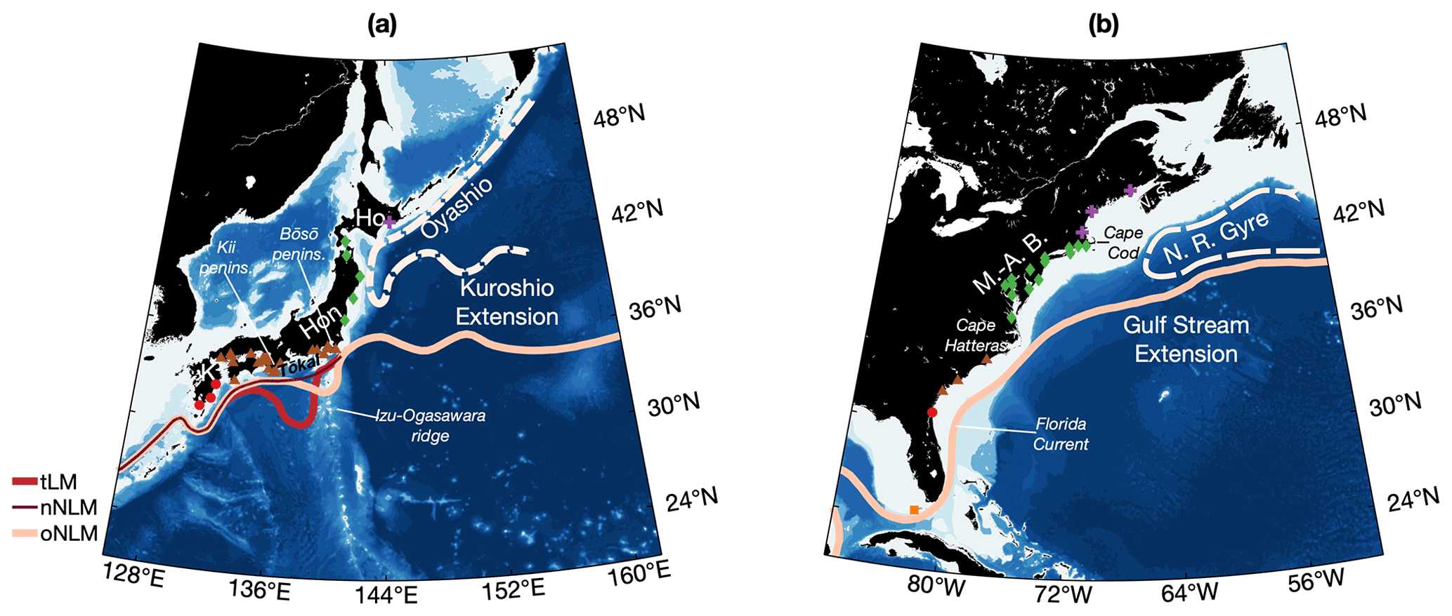
Figure 1(a) Kuroshio region circulation: the three Kuroshio paths – the typical large meander (tLM), the nearshore non-large meander (nNLM) and the offshore non-large meander (oNLM) are indicated upstream of the Izu–Ogasawara Ridge. The mean location of the KE is indicated offshore of this point, showing the location of the quasi-stationary meanders. The Oyashio current is shown in dashed pink. On land, K indicates Kyūshū, Hon stands for Honshū and Ho indicates Hokkaidō. (b) Gulf Stream region circulation from the Florida Current to the Gulf Stream Extension. The Northern Recirculation Gyre is also indicated. On land, MAB stands for Mid-Atlantic Bight and NS indicates Nova Scotia. Markers in (a) and (b) indicate the location of the tide gauges used in this study. The colour and shape of the markers in (a) and (b) indicate the angle used to rotate the wind stress in an alongshore and across-shore coordinate system for the removal of sea-level variability driven by local atmospheric effects (see Tables S1 and S2 in the Supplement). Shading in (a) and (b) indicates bathymetry.
Among the typical paths that the Kuroshio can take south of Japan (Fig. 1), the typical large meander is without doubt the most remarkable and is a major driver of the regional sea level (Kawabe, 2005, 1995, 1985) and atmospheric variability (Sugimoto et al., 2019). Large meanders (LMs) occur when two stationary eddies strengthen south of Japan. One is located southeast of Kyūshū and associated with an anticyclonic circulation; the other one is located south of Tōkai and associated with a cyclonic circulation. The front bounded by the two eddies becomes the Kuroshio large meander, and thus the cyclonic anomaly is inshore between the Kuroshio path and the southern coasts of Tōkai.
In the Atlantic, the Gulf Stream has its origins in the eponymous Gulf of Mexico, flowing past the Florida coastline as the Florida Current before leaving the boundary at Cape Hatteras near 35∘ N. From here it flows eastward as a meandering, eddying, free current in the Gulf Stream Extension and eventually the North Atlantic Current. From the American coast to 60–55∘ W, northward or southward lateral motions of the Gulf Stream Extension dominate its inter-annual and seasonal variability. This notable intrinsic variability closely follows the main mode of Atlantic atmospheric variability: the North Atlantic Oscillation (NAO) (Joyce et al., 2000; McCarthy et al., 2018). The abrupt transition from warm subtropical waters to cold subpolar waters marks a “North Wall” of the Gulf Stream (Fuglister, 1955). This Gulf Stream North Wall (GSNW) is a convenient marker of the lateral motions of the Gulf Stream Extension (Frankignoul et al., 2001; Joyce et al., 2000; Sasaki and Schneider, 2011b). The horizontal circulation of the separated western boundary current interacts with the vertical circulation. The vertical circulation in this region is part of the AMOC, which can be simplified as northward-flowing Gulf Stream waters and southward-flowing deep waters as part of the deep western boundary current (DWBC). One paradigm of the interaction of vertical and horizontal circulation in the region is that an enhanced DWBC and enhanced AMOC “push” the GSNW to the south and expand the Northern Recirculation Gyre (NRG). However, diverse behaviours have been found in models, with some supporting this paradigm (Zhang and Vallis, 2007; Zhang, 2008; Sanchez-Franks and Zhang, 2015) and some finding the opposite: an enhanced AMOC and northward-shifted GSNW (De Coetlogon et al., 2006; Kwon and Frankignoul, 2014). Alternatively, as in the Pacific with the KE, the Gulf Stream Extension has been linked to the mechanism of remote wind stress curl forcing the westward propagation of large-scale jet undulations (Sasaki and Schneider, 2011b; Sirven et al., 2015). Finally, Andres et al. (2013) highlighted the fact that the coastal sea level on the large shelf north of Cape Hatteras was in agreement with the location of the Gulf Stream Extension west of 69∘ W and suggested that the shelf transport pushes the Gulf Stream, whereas Ezer et al. (2013) hypothesized that a more inertial Gulf Stream south of the separation point may “overshoot” to the north when leaving the coastline at 35∘ N and control, at least to some extent, the location of the extension.
The diversity of proposed driving mechanisms of the Gulf Stream Extension meridional shifts may be explained by the great spatial differences over short distances along the Gulf Stream Extension. Indeed, some factors induce incongruity in the along-jet variability of the Gulf Stream Extension. This is the case of the time-dependent flanking cells of the Gulf Stream, which are recirculations located immediately downstream of Cape Hatteras and which induce along-stream decorrelation in the Gulf Stream Extension surface transport (Andres et al., 2020). This indicates that different mechanisms are acting on the position of the Gulf Stream Extension. The aforementioned hypotheses for meridional shifts of the Gulf Stream Extension are hence not necessarily mutually exclusive and may co-exist at different downstream distances from Cape Hatteras.
While the Gulf Stream and Kuroshio are western boundary currents driven by the closure of the Sverdrup balance (Stommel, 1948; Munk, 1950), even the brief introduction presented here highlights both differences and similarities between the currents. Upstream of the separation points, the currents behave quite differently. The Kuroshio takes a number of distinct paths, whereas the Gulf Stream hugs the coast tightly. The separation points at the Bōsō peninsula and Cape Hatteras both have a remarkably similar latitude at 35∘ N. Downstream, the Gulf Stream Extension flows northeastward, whereas the Kuroshio Extension mainly flows eastward. The meandering of the Kuroshio in its extension region is much more defined than that of the Gulf Stream Extension, with no named quasi-stationary meanders in the Gulf Stream Extension (until farther downstream at the Mann eddy). The north–south shifts of the extensions are remarkable features of both basins and account for an important part the extensions' variability. It is well established that these lateral shifts are caused by the propagation of long jet-trapped waves forced by downstream wind in the Pacific, whereas the mechanisms driving the GSNW are not completely clear, with a plausible role of a similar mechanism of wind-forced jet undulation. These jet-trapped waves are possible thanks to the sharp gradient of relative vorticity induced by WBC extensions comparable to or greater than the meridional gradient of planetary vorticity within the mid-latitude band. Hence, the jet-trapped waves are essentially Rossby waves, but they propagate in the waveguide formed by the WBC extension, which allow their meridional narrowing as they progress westward and their southwestward propagation in the Atlantic (Sasaki et al., 2013; Sasaki and Schneider, 2011a, b; Sirven et al., 2015). It is, however, important to note that, in the Atlantic, the lateral shifts of the Gulf Stream Extension have been more often linked with the DWBC and the NRG. In the Pacific, southern (northern) shifts of the Kuroshio Extension are known to be concurrent with periods of instability (stability), whereas, until recent years (prior to ∼2000), the Gulf Stream Extension has been much more stable (Andres, 2016; Gangopadhyay et al., 2019). The interaction with the cold currents to the north is also quite different. The continent north of the Gulf Stream to Newfoundland lends to a topographical constraint on the gyre circulation, whereas the Oyashio is much less constrained by land. Conversely, the upstream Kuroshio is much more constrained than the upstream Gulf Stream due to the presence of the Izu–Ogasawara Ridge. Additionally, there is no Pacific equivalent to the coastal circulation on the prominent shelf north of Cape Hatteras (Peña-Molino and Joyce, 2008). The AMOC is a notably Atlantic-specific feature, but there is not a distinct feature of the horizontal circulation that clearly identifies with the presence of the AMOC in the Atlantic basin that is not present in the Pacific basin. While a decline in the AMOC is robust in climate projections and will weaken the Gulf Stream (Chen et al., 2019), WBCs are also expected to change. The Kuroshio is expected to strengthen because of sea surface warming (Chen et al., 2019). WBCs have been observed to be shifting polewards (Wu et al., 2012; Stocker et al., 2013) and becoming more unstable (Andres, 2016; Beal and Elipot, 2016; Gangopadhyay et al., 2019).
Tide gauges (TGs) estimate relative sea level at the coast and have done so since the 18th century in certain locations (e.g. Amsterdam, Stockholm, Kronstadt, Liverpool, Brest). Tide gauges have long been used to investigate ocean circulation in regions such as the Gulf Stream where the impact of strong ocean circulation on coastal sea level is apparent (Montgomery, 1938). However, ocean circulation is far from the only impact on sea level at the coast. The effects of land motion (including glacial isostatic adjustment), thermosteric expansion, terrestrial freshwater changes (including river runoff and ice melt) and gravitational fingerprints all feature in sea-level variations at the coast (Meyssignac et al., 2017). In addition, the local forcing of the atmosphere drives an important part of the coastal sea-level variability, particularly in shelf environments. Variations in wind stress can force water to travel toward (or away from) the coastline, consequently raising (lowering) the sea level at tide gauge locations. Both across-shore and alongshore wind stresses can impact sea level, as can variations in the local air pressure through the inverse barometer (IB) effect. On the American northeast coast, the inverted barometer greatly influences inter-annual change in the mean sea level, dominates most extreme inter-annual changes and is not negligible on multidecadal timescales (Piecuch and Ponte, 2015), while the alongshore wind is also believed to play a role (Andres et al., 2013; Woodworth et al., 2014; Piecuch et al., 2019). This contribution of the atmosphere to the mean sea level is particularly challenging to disentangle from the contribution of ocean dynamics because the two share a similar range of timescales. Hence, great care is needed to interpret coastal sea-level fluctuations measured by tide gauges as representative of ocean circulation patterns.
A number of approaches have been developed to investigate ocean circulation using tide gauge data. The cross-stream gradient of sea level can be estimated by using an onshore tide gauge and an offshore island tide gauge (Montgomery, 1938; Kawabe, 1988; Ezer, 2015; Marsh et al., 2017), providing a direct estimate of a boundary current flowing between the gauges via the geostrophic relationship. This type of estimate is restricted to locations where suitable offshore island tide gauges exist. Apart from the limited number of such locations, the offshore estimate is located in the eddy-filled ocean interior, which can experience sea-level fluctuations driven by the ocean mesoscale (Sturges and Hong, 1995; Firing et al., 2004) that are not representative of the large-scale ocean circulation. In the Atlantic, a number of studies (e.g. Bingham and Hughes, 2009; Ezer, 2013; McCarthy et al., 2015) have used long tide gauge records to estimate the strength of the AMOC, which has only been continuously observed since 2004 (Cunningham et al., 2007). In the Pacific, the difference between the sea level either side of the Kii peninsula (Fig. 1) has been extensively used to diagnose past occurrence of the typical large meander (Moriyasu, 1958, 1961; Kawabe, 1985, 1995, 2005), despite the causal relationship not being fully understood.
Recent advances have been made on the theoretical underpinning of the relationship between sea level at the western boundaries of the ocean and the offshore processes that influence sea-level fluctuations (Minobe et al., 2017; Wise et al., 2018). The rule of thumb of Minobe et al. (2017) for a western boundary of the Northern Hemisphere is as follows: the sea level at a point on the coastline is influenced by (1) long Rossby waves (or any other mass input from the east) incident on that point and (2) coastally trapped waves transmitting the sea-level signal equatorward from points farther to the north, which can equally be influenced by incidental long Rossby waves. It follows that the alongshore gradient of the coastal sea level at a given latitude is proportional to the sea-level input from the east at the same latitude (Minobe et al., 2017):
where ζ is the sea-level anomaly evaluated at the coast (xW) and at the frontier between the boundary layer and the ocean interior (xI), and β is the meridional gradient of the Coriolis frequency f. In the real ocean, the mass input into the western boundary region is more accurately described by the jet-trapped Rossby wave framework than by the direct westward propagation of linear long Rossby waves (Sasaki et al., 2013; Sasaki and Schneider, 2011a; Taguchi et al., 2007). Therefore, pairing the jet-trapped theory with the Minobe et al. (2017) framework is expected to better estimate the sea level on the coast of western boundaries. In accordance with this idea, the coastal sea level south of Japan is known to be in agreement with the Kuroshio location above the Izu–Ogasawara Ridge (Kuroda et al., 2010), the KE meridional shifts during the satellite era (Sasaki et al., 2014) and the regime shifts in North Pacific mid-latitude (Senjyu et al., 1999). Simply put, the mechanism is that jet-trapped long waves, originating from the east and responsible for the meridional shifts of the WBC extension, break when reaching the coastline into coastally trapped waves that propagate equatorward (Sasaki et al., 2014). Similarly, two very recent studies pointed towards an agreement between the Gulf Stream Extension variability and the sea-level change south of Cape Hatteras (Dangendorf et al., 2021; Ezer, 2019). This link is not yet well known or understood in the Atlantic basin and deserves to be furthermore explored.
Globally, the mean sea level has shown an increased rate of rise in the last decades (Dangendorf et al., 2019; Nerem et al., 2018) induced by anthropogenic emission of greenhouse gases in the atmosphere, which is a major issue for coastal communities and environments. Understanding the relationship between sea level and ocean circulation is a component of understanding coastal vulnerability to changing sea levels. Many densely populated regions border WBCs, and large changes in WBCs could have big sea-level impacts. In the Northern Hemisphere, the Gulf Stream and Kuroshio border the US and Japanese eastern seaboards, two of the most densely populated coastlines in the world.
Links between the coastal sea level of western boundaries and the nearby ocean dynamics have rarely been compared between basins. Chen et al. (2019) addressed projected sea-level changes through the 21st century in both Kuroshio and Gulf Stream regions in the context of global warming and AMOC weakening. Ezer and Dangendorf (2021) focused on the energy budget of the western boundary regions. Here, we analyse datasets of mean sea level along US and Japanese eastern coastlines, identify major spatial modes of variability, and interpret this in terms of ocean circulation variability. We explore the statistical links between the sea-level changes and the western boundary current extension variability. This paper is organized as follows. Section 2 presents the data used in this study and the derivation of indices for the WBC extensions. The results of the analysis of the gauge records and their relationship to upstream and downstream WBC variability are presented and discussed in Sects. 3 and 4. A conclusion is presented in Sect. 5.
2.1 Tide gauge selection, treatment and adjustment for surge variability
Tide gauge data were obtained from the Permanent Service for Mean Sea Level (Holgate et al., 2013, PSMSL, 2020, https://www.psmsl.org/, last access: 18 October 2021) on 17 August 2020. We selected tide gauge stations along the western boundary of the North Atlantic, on the coast of the United States and Canada, and along the western boundary of the North Pacific on the coast of Japan. To retain only measurements of sufficient quality, length and completeness, historical series with more than 10 % of missing monthly values as well as those flagged for quality issues are excluded. Consequently, the number of individual tide gauge records available is dependent on the chosen period. A summary of gauge details is given in Tables S1 and S2 in the Supplement.
For the Atlantic, the period considered is January 1948–December 2019 due to the availability of the atmospheric reanalysis used to correct for surge effects. The island station on Key West is located onshore of the Gulf Stream and features a signal coherent with the Florida tide gauges. It is therefore included, leaving a total of 22 stations on the American east coast.
The Japanese tide gauge network is more recent; therefore, the period considered for the Pacific is January 1968–December 2019. The records of most stations on the eastern coast of Honshū feature important offset shift and/or drift after the March 2011 tsunami and cannot be used as such, leaving a ∼700 km coastline strip depleted of any measurement. To remedy the issue, we retained the three long records of Onahama, Miyako II and Ayukawa and replaced existing or missing data after February 2011 with the closest SSH measurement with trend and offset adjustment. The total number of tide gauges retained for the Pacific region is 30 after the criterion of completeness is applied.
Missing values are linearly interpolated for both regions. No adjustment for long-term processes affecting the sea level is performed as the records are quadratically detrended. Monthly anomalies are obtained by subtracting the climatological monthly mean.
To correct the records for the effect of local winds and pressure, monthly sea-level pressure and 10 wind speeds were obtained from the NCEP/NCAR Reanalysis 1 (Kalnay et al., 1996, NOAA/OAR/ESRL PSL, https://psl.noaa.gov/, last access: 18 October 2021). They are available from 1948 to the present day. The grid has a resolution of 1.875∘ in longitude and ∼1.904∘ in latitude. The variables are detrended and deseasonalized after the wind speed is converted to wind stress. The Japanese 55-year Reanalysis (Kobayashi et al., 2015, JRA-55, https://jra.kishou.go.jp/index.html, last access: 18 October 2021), available from 1958, was also retrieved. Results were similar to those obtained with the NCEP variables and are therefore not discussed. To assess and remove the local atmospheric contribution to changes in sea level, each monthly sea-level record is regressed against the atmospheric pressure and the wind stress interpolated at the gauge location, following the method of Dangendorf et al. (2013, 2014), Frederikse et al. (2017) and Piecuch et al. (2019). Details are given in Appendix A, together with a brief analysis of the results. We find that the local forcing of the atmosphere drives between 30 % and 50 % of the monthly sea-level variability at tide gauges located north of Cape Hatteras, the separation point of the Gulf Stream, and at tide gauges located north of 38∘ N on the eastern coast of Japan, whereas the atmospheric influence is reduced upstream of the separation points of the Kuroshio and Gulf Stream. The unexplained residual represents the sea level corrected for local atmospheric effects.
Finally, to focus on inter-annual and slower variations, a low-pass 19-month Tukey filter is applied. The filtering effectively reduces the period analysed to November 1968–January 2019 for the Japanese gauges and November 1948–January 2019 for the American gauges.
2.2 Additional datasets
Gridded monthly sea surface height (SSH), temperature (SST) and velocities (SSVs) derived from satellite altimetry are available from 1993 and were obtained from the Copernicus Marine Environment Monitoring Service (CMEMS) website (https://marine.copernicus.eu, last access: 18 October 2021). They are obtained from the ARMOR3D product (Guinehut et al., 2012; Mulet et al., 2012). The three datasets have a regular grid of .
To examine the variability of the Gulf Stream extension and the Kuroshio extension, the EN4 quality-controlled subsurface (200 m depth) ocean temperature profiles (Good et al., 2013, EN4.2.1) are used. The 1981–2010 objectively analysed mean temperature at 200 m depth field from the World Ocean Atlas 2018 (Locarnini et al., 2018, WOA18) is used to derive the climatological position of the Gulf Stream and Kuroshio extensions between 75 and 55∘ W and between 141 and 161∘ E, respectively. The climatological extension positions are defined as the whole-number isotherm roughly corresponding to the surface velocity maximum, which is 17 ∘C in the Atlantic and 16 ∘C in the Pacific. The two datasets were downloaded on 8 September 2020. Derivation of jet latitudinal position indices is detailed in Sect. 2.3
Finally, we retrieved additional indices that infer oceanic and atmospheric variability. We make use of the GSNW index from Joyce et al. (2000) and of the Kuroshio Extension indices from Qiu et al. (2016), and we also derive indices for the variability of the two WBC extensions in Sect. 2.3. Additionally, the estimate of the southernmost latitude of the Kuroshio axis south of Tōkai (136–140∘ E) produced by the Japan Meteorological Agency (JMA) was retrieved from their website (https://www.data.jma.go.jp/gmd/kaiyou/data/shindan/b_2/kuroshio_stream/kuro_slat.txt, last access: 18 October 2021). This index represents the upstream meridional movements of the Kuroshio south of Japan. We also retrieved the monthly North Atlantic Oscillation (NAO) index from James Hurrell and the National Center for Atmospheric Research Staff (Eds) NAO web page (https://climatedataguide.ucar.edu/climate-data/hurrell-north-atlantic-oscillation-nao-index-station-based, last access: 18 October 2021).
As the tide gauge records and the reanalysis variables, satellite observations are deseasonalized, detrended and filtered with a 19-month Tukey filter, unless otherwise mentioned. All aforementioned indices are similarly deseasonalized, detrended and filtered, with a couple of exceptions: yearly indices cannot be filtered at such a high cut-off frequency, and the indices of Qiu et al. (2016) feature no seasonal variability and are therefore not deseasonalized.
The significance of correlations between two time series A and B is calculated using the non-parametric method of Ebisuzaki (1997), as was previously done in McCarthy et al. (2015). The method consists of evaluating the Fourier transform of A and generating a large number (here 5000 is used) of random time series with similar spectral properties. The modulus is preserved while the phase is randomized. The randomly generated signals are then correlated against B. Significance for zero lag correlation between A and B is given as the percentage of randomly generated correlations which are less than the correlation between A and B (using absolute values). When we report lagged correlations, we use a more stringent test of confidence, as in McCarthy et al. (2015). In this case, the lead–lag correlation between each randomly generated signal and B is computed, and the maximum correlation is determined. The significance is given as the percentage of randomly generated maximum correlations which are lower than the maximum correlation between A and B (within the limit of a lead or lag of a fourth of A or B length).
2.3 Meridional motions of the western boundary current extensions
At inter-annual to multidecadal scale, the Gulf Stream Extension and the Kuroshio Extension are quite similarly characterized by strong lateral movements. The displacements are of about half a degree in the Atlantic (Joyce et al., 2000) and about 1∘ in the Pacific (Sasaki et al., 2013), with an increase in the meridional extent of the shifts toward the east.
For each ocean, the methods used to quantify such oscillations have evolved differently. In the North Atlantic, the Gulf Stream North Wall (GSNW) is defined as the leading mode of the temperature anomaly at the climatological position of the jet or, more traditionally, its northern front (the North Wall). Indeed, because the WBC extensions separate cold water to the north from warm water to the south, warming (cooling) at the climatological jet position reflects a northern (southern) shift of the jet. In the Pacific, recent work has used SSH estimates averaged in the 31–36∘ N and 140–165∘ E box as proxy to infer the past Kuroshio Extension meridional location (Qiu et al., 2014, 2016). This area corresponds to the Kuroshio Southern Recirculation Gyre (KSRG), the strength of which is a good indicator not only of the Kuroshio Extension latitudinal location, but also of its stability and intensity (Qiu et al., 2014).
To produce consistent indices for both oceans, we made use of the subsurface sparse temperature observations to derive up-to-date indices of the meridional location of the Kuroshio Extension and Gulf Stream Extension, following the GSNW calculation method of Sasaki and Schneider (2011b) and Frankignoul et al. (2001). Given the data availability, the analysis period was restricted to 1960 and 1965 onwards for the Atlantic and Pacific, respectively. For each year up to 2019, the available sparse subsurface temperature observations were interpolated at the climatological position of the Gulf Stream and Kuroshio extensions using an inverse distance-weighting technique with power parameter p=2 and a search radius of 400 km, allowing construction of an along-jet temperature matrix. The search radius acts as a spatial low-pass filter and was purposely set well above the Rossby deformation radius to minimize the mesoscale meandering variability in the gridded temperature anomaly. The leading mode of variability is extracted for each basin by performing an empirical orthogonal function (EOF) decomposition based on correlation (rather than covariance) on the detrended temperature anomaly. Figure 2 presents the associated EOFs (a and b) and principal components (c and d, light blue lines) for the Atlantic and the Pacific, respectively. The EOF amplitude in both oceans varies in-phase all along the climatological jet axis. In the remainder of this paper, we refer to the principal components as the GSNW and KE index (KEI), and we specify “this study/our GSNW” or “this study/our KEI” whenever precision is needed.
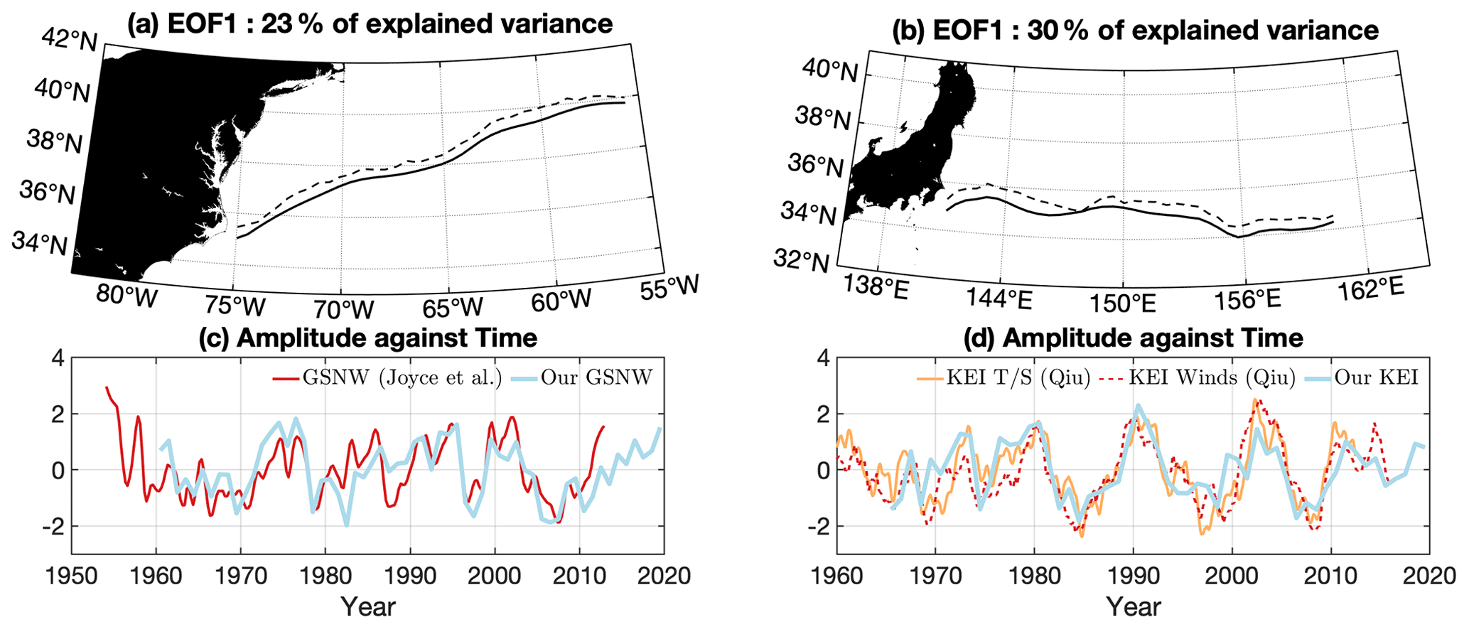
Figure 2(a) GS climatological position (solid line) and GS climatological position plus GSNW spatial amplitude based on EOF analysis of the along-jet temperature anomalies (dashed line). Conversion ratio from normalized temperature to latitude is arbitrarily set for visualization but is the same at every grid point. (c) GSNW time series obtained from EOF analysis (thick light blue), with the GSNW index of Joyce et al. (2000) also shown in red. Panels (b) and (d) are as for (a) and (c) but obtained for the Kuroshio Extension and with the KE indices of Qiu et al. (2016) replacing Joyce et al. (2000). The solid orange line in (d) corresponds to the temperature- and salinity-based index, and the dashed thin red line corresponds to the wind-based index. All time series in (c) and (d) are normalized.
To contextualize the temporal variations of our GSNW and KEI with existing indices, we compared the GSNW estimate of Joyce et al. (2000), available from 1955 to 2011, and the two KEIs of Qiu et al. (2016). The KEIs of Qiu et al. (2016) are derived from the KSRG strength as mentioned above and were initially introduced by Qiu et al. (2014) using satellite altimetry and model output. They have recently been made available from 1905 to 2015 (1945 to 2012) using wind (temperature salinity) data (Qiu et al., 2016). The wind-based index is obtained by forcing a 1.5-layer reduced-gravity model with historical wind stress merged from the ERA-20C and ERA-Interim reanalysis sets. Although such a model has limited skills in reproducing the westward narrowing of the meridional jet oscillations (see Sasaki et al., 2013; Sasaki and Schneider, 2011a), it is able to correctly match the timing of the KE meridional shift (Taguchi et al., 2007). The three indices are presented alongside the GSNW (this study) and KEI (this study) in Fig. 2c and d after detrending is applied. They are annually averaged for comparison with our GSNW and KEI. Correlations between both Qiu et al. (2016) indices and our KEI are high, with a greater value obtained with the T S index (r=0.75, significance is above 99 %) than with the wind-based index (r=0.67, significance is 99 %). Similar correlation is found between the Joyce et al. (2000) GSNW and the GSNW from this study over their overlapping period: 0.71 (significance >99 %).
In this section, we propose scrutiny of the inshore sea level measured by tide gauges using cross-correlation and moving correlation analysis, as well as empirical orthogonal function (EOF) analysis. We relate the obtained spatial and temporal patterns to ocean circulation. Senjyu et al. (1999), Valle-Levinson et al. (2017) and Sasaki et al. (2014) used EOF decomposition on the Pacific and the Atlantic tide gauges, and hence our analysis can be seen as building on their work.
3.1 Cross-correlation analysis
Correlation analysis has been performed extensively for tide gauges on the US east coast from Woodworth et al. (2014), McCarthy et al. (2015), Piecuch et al. (2016) and Calafat et al. (2018), among others. The resultant correlation patterns suggest groupings of tide gauges across geographic regions, with boundaries defined by changing oceanographic circulation regimes, which we argue are the fingerprints of ocean circulation on coastal sea level.
We expand the analysis to tide gauges along the Japanese coast. Three tide gauge groupings are apparent in Fig. 3a based on the cross-correlation between Japanese records. West of the Kii peninsula, the correlation between gauges is on average 0.85. From the Kii peninsula to the Bōsō peninsula region, which we refer to as Tōkai for simplicity, another highly correlated group exists. The mean of the correlations within that group is 0.74, with the tide gauge of Owase (tide gauge 18) showing slightly lower agreement. These two groups south of Japan were identified by the early work of Moriyasu (1958). The gauges on the eastern coastline of Honshū and Hokkaidō, including the tide gauge of Katsuura (TG 24) east of the Bōsō peninsula, show lower correlation with each other and are referred to as the Oyashio group. The limits of the correlation groupings match two oceanographic boundaries: the Kii peninsula, where the Kuroshio detaches during large meander periods, and the region of the Bōsō peninsula, where the Kuroshio leaves the coast to become the Kuroshio Extension (see Fig. 1).
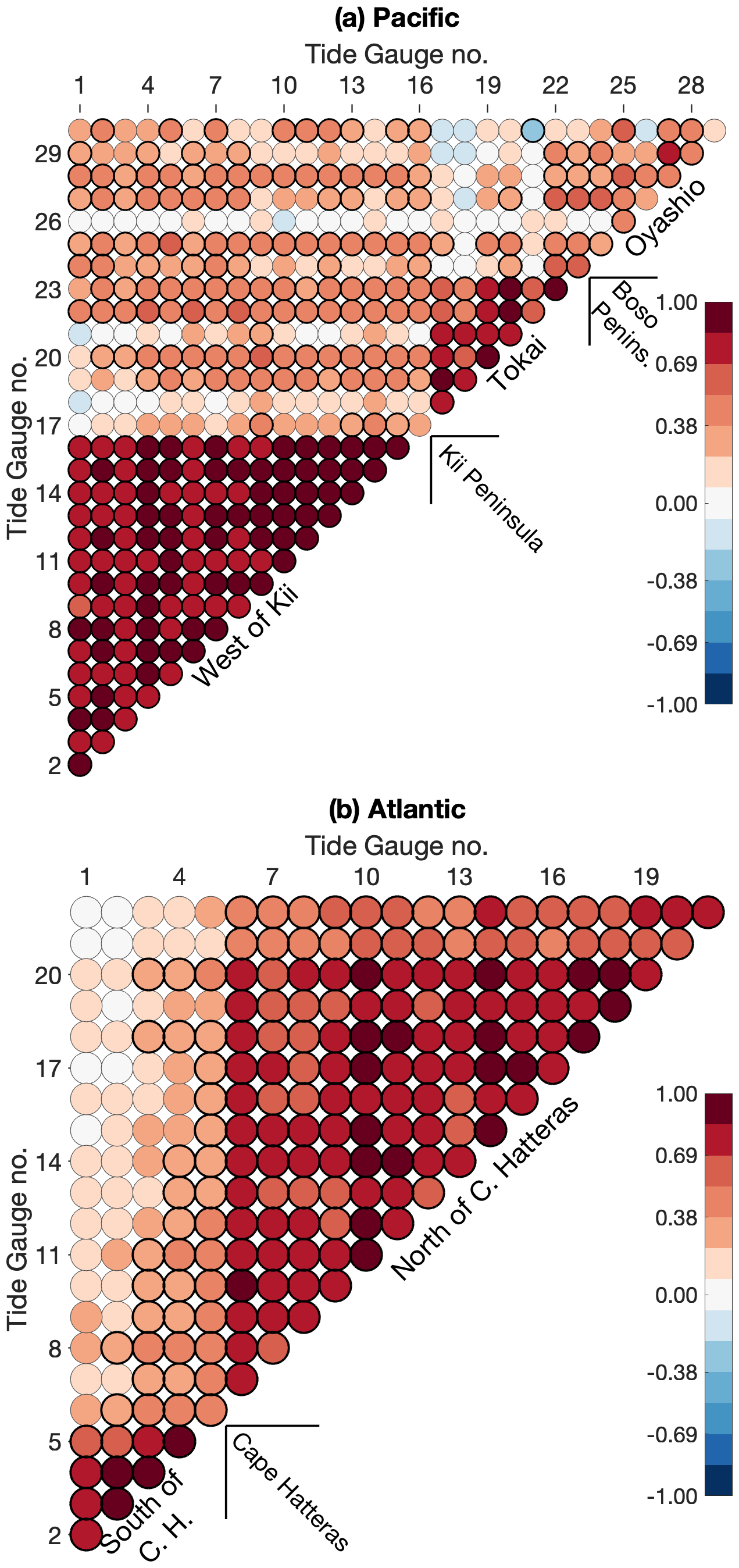
Figure 3(a) Pacific and (b) Atlantic tide gauge cross-correlation at zero lag. Each circular marker gives the correlation rij between gauge i and gauge j. Tide gauges are numbered in ascending order from south to north, following the coastline (a list is given in Tables S1 and S2 in the Supplement). The bolder circular contour indicates that the correlation is above a significance level of 95 %.
In the Atlantic, the pattern of correlation previously highlighted by McCarthy et al. (2015) and Woodworth et al. (2014) of a drop in correlation between tide gauges north and south of Cape Hatteras – the point at which the Gulf Stream leaves the coastline – is also seen in our analysis, with a distinct change in correlation patterns noted either side of Cape Hatteras (Fig. 3b). All gauges south of Cape Hatteras display almost identical behaviour, with a correlation average within that group equal to 0.78. All the gauges north of Cape Hatteras display high correlations as well: on average 0.72. The correlation of the three gauges located north of Cape Cod with the others north of Cape Hatteras is lower (on average r=0.64, including the tide gauge of Boston, TG 20, and r=0.58 without). This indicates that another boundary exists at Cape Cod, although the transition is not as abrupt as across Cape Hatteras. Despite the tide gauges being instruments locked at the coast, the obtained correlation patterns are representative of the two-dimensional sea-level coherence above the shelf. Indeed, similar groupings are visible in SSH data, extending from the coast to the shelf edge and featuring similar boundaries between one another (Cape Hatteras and Cape Cod; see Fig. 2 in Ezer, 2019).
In the Atlantic, Thompson and Mitchum (2014), Frankcombe and Dijkstra (2009), and Häkkinen (2000) noted high correlation of sea-level variations from Nova Scotia (Canada) to the Caribbean. This, of course, implies correlation across Cape Hatteras. While we do find a few significant correlations at the 95 % level across Cape Hatteras, indicated by bold outlines in Fig. 3, the distinct drop in correlation is more prominent. We therefore investigate the evolution of the correlation patterns through time in Figs. 4 and S1 in the Supplement. Within the groups (a) south and (b) north of Cape Hatteras, the individual correlations (Fig. S1a and b in the Supplement, thin grey lines) are high and show little time dependency, with the median never dropping below 0.54 south of Cape Hatteras and below 0.65 north (solid red lines). Figure 4b shows the changing correlations between gauges located on either side of Cape Hatteras (thin grey line) and the moving correlation between the two grouping averages. The correlations are high and the moving correlation between the two grouping averages is significant most of the time from roughly the 1950s to the late 1980s, when the correlations drop abruptly. From the 1990s onwards, there is no correlation between the two regions, with the exception of the most recent era from approximately 2010, when the correlation is negative. This change in behaviour was also noted by Kenigson et al. (2018) (see their Supplement).
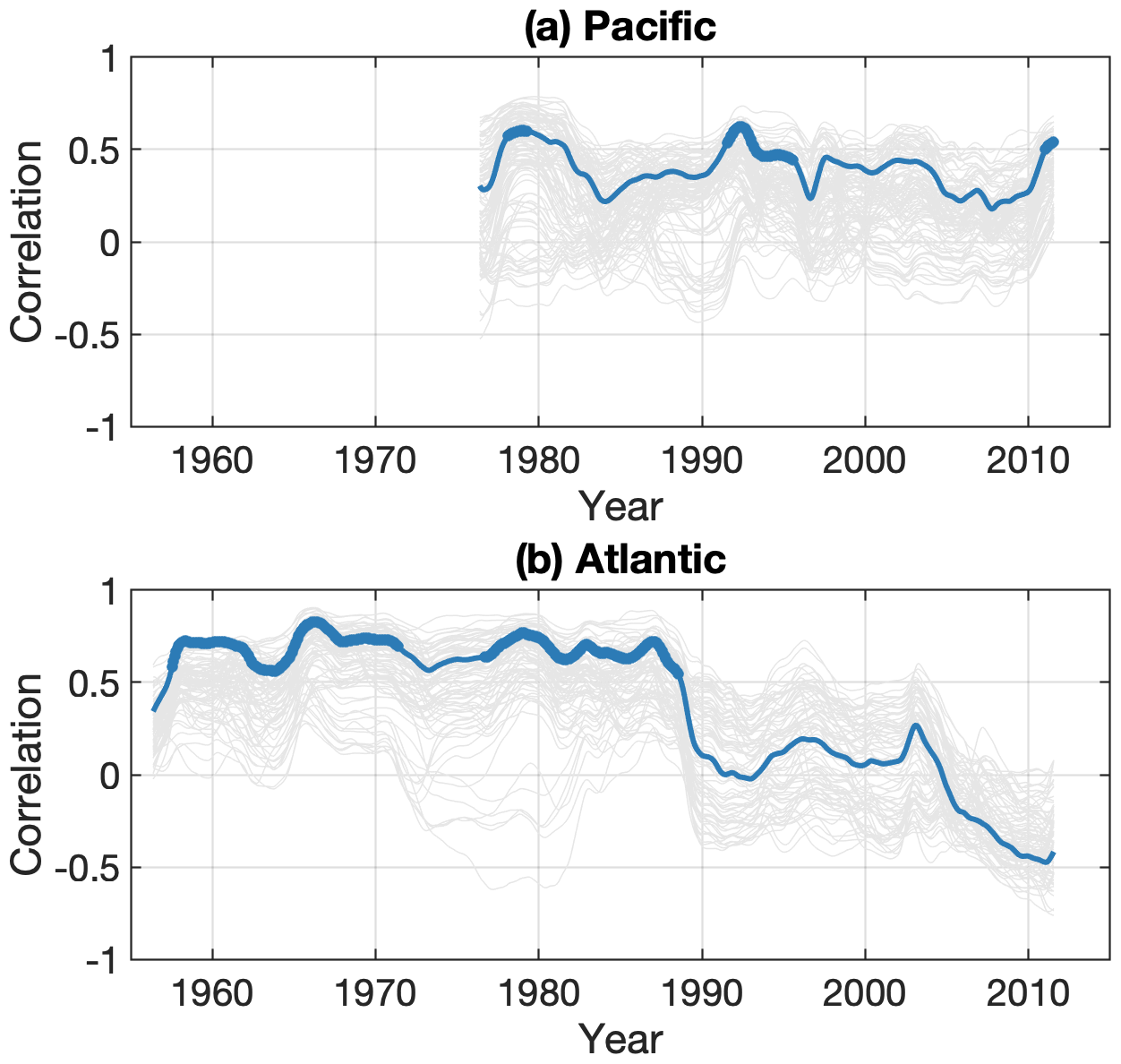
Figure 4Moving correlation analysis between tide gauge records with a running window of 15 years. Each individual grey line renders the moving correlation between two records. The x axis represents the centre of the moving window. (a) Cross-correlation between the Oyashio group and west of the Kii group (grey lines). (b) Cross-correlation between gauges on either side of Cape Hatteras, the separation point of the Gulf Stream (again, grey lines). In each panel, the solid blue line is the moving correlation between the group average of sea-level anomalies. Significant correlations above the 95% level are indicated by a thicker blue line.
In the Pacific, the correlations within the two southern groupings feature little temporal variation (Fig. S1c and d in the Supplement). The large deviations between individual correlations within the Oyashio group underline the overall lower agreement between the gauges there (panel e). As will be discussed further below, the sea level south of Tōkai is largely affected by the appearance of large meanders, which is a phenomenon unique to the Pacific. Thus, to compare southern and northern variability as was done for the Atlantic in Fig. 4b, we plotted the changing correlations between the group west of Kii and the Oyashio group in Fig. 4a. The correlations are relatively low over the whole period, with the correlation median exceeding r=0.35 only on three occasions: 1978–1982, 1991–1993 and 2011–2012 (not shown). The moving correlation between the two grouping averages is rarely significant except in the early 1990s. More importantly, the moving correlations do not show an abrupt change, in contrast to the situation in the Atlantic.
3.2 Empirical orthogonal function analysis
We employ empirical orthogonal function (EOF) analysis to objectively reduce the sea-level anomalies in an ensemble of modes, each composed of a time-varying coefficient α, the principal component (PC) and associated spatial-varying coefficients ϕ, the empirical orthogonal vector or function (EOF). Covariance-based EOF decomposition is performed on tide gauge sea-level anomalies interpolated on a regular grid. This prevents the sea-level variability in better-sampled regions from being favoured in the analysis. Details of the interpolation on a regular grid, including handling of estuarine stations, are given in Appendix B. The regular grid points are referred to as virtual stations.
The EOF analysis is computed separately on both Atlantic and Pacific gridded sea-level anomalies. Together, the two leading modes explain 85 % (77 %) of the variability of the Atlantic (Pacific) dataset.
3.2.1 Atlantic and Pacific first modes
The leading mode of the Pacific dataset explains 47 % of the overall variance. The associated EOF, ϕ1, features a common region of coherence west of the Bōsō peninsula, south of Japan, where the Kuroshio separates from the coast (Fig. 5a, circular markers). The Atlantic leading mode explains 60 % of the variance, and, in a similar way, ϕ1 features greater amplitudes south of the separation point at Cape Hatteras, decreasing northward from there (Fig. 5b).
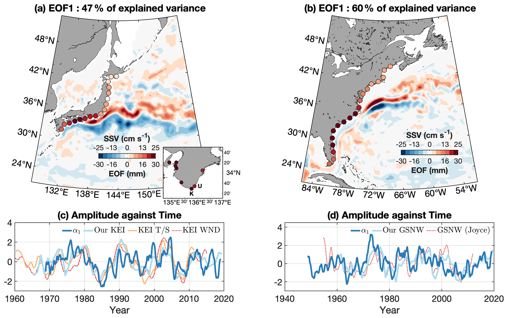
Figure 5The leading EOF (ϕ1) of the gridded tide-gauge-based sea-level anomaly (circular markers) from the Pacific (a) and the Atlantic (b). The associated principal components α1 are shown as thick dark blue lines for the Pacific (c) and Atlantic (d), together with indices of the WBC extension meridional location: this study (thick light blue line), Qiu et al. (2016) T S-based (thin orange line) and wind-based (thin dot-dashed red line) KEIs, and Joyce et al. (2000) GSNW (thin red dot-dashed). All time series in (c) and (d) are normalized. For each basin, colour shading in (a) and (b) is the sea surface velocity magnitude composite difference based on the principal component α1 (period of minus period of ). The arbitrary threshold of was used, but taking any number between 0 and 1 leads to similar patterns. The inset in (a) presents the regression coefficient obtained when the principal component is regressed on the original tide gauges, with a zoom-in on the Kii peninsula.
On the southern coastline of Japan (130–141∘ E), the amplitude is on average 2.3 cm (excluding the easternmost virtual station located on the Bōsō peninsula; ϕ1=0.7 cm). Towards the north, east of Honshū and Hokkaidō, the mode amplitude is reduced by a factor of 3 and equals 0.7 cm on average (this time including the virtual station on the Bōsō peninsula). The mode temporal variations α1 are presented in Fig. 5c. There is a decrease from the late 1970s to 1985, followed by an increase until 1990. From there onwards, the principal component exhibits marked fluctuations with a 4–7-year period. In the Atlantic, the transition from the south of Cape Hatteras, where ϕ1 is on average 2.6 cm, to the north where it is on average 1.3 cm is not as pronounced as with the Pacific gauges. The associated time-varying amplitude α1 was maximum in the mid-1970s, the mid-1980s and the early 1990s, and it was particularly low in the mid-1960s, the early 1980s and the 2000s (Fig. 5d).
To demonstrate the link between the gauge records and the ocean dynamics, we computed two composites using the monthly surface velocity magnitude since the beginning of that record in 1993 (Mulet et al., 2012). The surface velocity magnitudes are averaged over periods of strongly positive α1 (greater than two-thirds its standard deviation, i.e. ) to form a first composite, and a similar procedure is done over periods of strongly negative α1 (lower than minus two-thirds its standard deviation, i.e. ). The threshold of is arbitrary, but taking any other thresholds within 0–1 leads to similar patterns. For each basin, colour shading in Fig. 5a–b represent the difference between sea surface velocity composites based on each mode temporal amplitude.
Similar patterns are seen in both basins downstream of the separation points. In the Pacific, the positive velocities east of the ridge (>140∘ E) are located farther north than the negative velocities, indicating that the Kuroshio Extension is found more to the north during the period of positive α1. The surface velocity composite in the Atlantic presented alongside the EOF in Fig. 5b highlights an analogous situation, with the Gulf Stream Extension drifting to the north (positive velocity pattern) during periods of strong positive α1 (early 1990s, mid-2010s) and to the south (negative velocity pattern) during periods of strong negative α1 (2000s).
Different patterns are found upstream of the separation point. South of Japan and east of 136∘ E, a region of positive velocity exists close to the coast, to the north of negative velocities. In particular, in the Izu–Ogasawara Ridge region (140∘ E), positive velocities are above the deep channel located north of 34∘ N (deeper than 1500 m), whereas negative velocities are spread above the shallower part of the ridge to the south (shallower than 1500 m). The Kuroshio south of Tōkai was hence found northward (southward) during periods of positive (negative) α1. Moreover, it is obvious that the positive velocity pattern (associated with high α1) resembles the nearshore NLM (see Fig. 1), whereas the negative velocity pattern (associated with low α1) resembles the offshore NLM, which is a finding consistent with Kawabe (1989). In the Atlantic, the negative velocity pattern is inshore of the positive velocity pattern upstream of Cape Hatteras, indicating that during periods of positive (negative) α1, the upstream Gulf Stream was offshore (inshore).
To extend the analysis of the relationship between the two principal components and the extension location prior to the satellite era, we make use of the Kuroshio Extension indices and Gulf Stream North Wall indices (this study; Qiu et al., 2016; Joyce et al., 2000) described in Sect. 2. The principal components are correlated against the indices after they were yearly or quarterly averaged (when necessary). There is moderate but significant correlation between the Pacific α1 and the various KE indices. The maximum correlation with our KEI (Fig. 5c, solid green curve) is r=0.52 (significance is 99 %) and is found at zero lag. Similarly, we obtain moderate correlation between α1 and the two Qiu et al. (2016) indices. There is better agreement with the index based on temperature and salinity (Fig. 5c, orange line), with r=0.52 when α1 leads by 1 month (significance is 99 %; note that r=0.52 for leads between 0 and 2 months, with similar significance), than with the wind-based index (dot-dashed red line), for which the correlation maximum is found when α1 lags by 7 months and is r=0.41 (61 %). The correlation is not stationary through time, however. The 1990s are a period of lesser agreement, as the sea-level features a bump which is not seen in KEIs. In contrast, the signals co-vary from 2000 onwards. Likewise, they all feature the strong shift of the late 1970s to mid-1980s.
Correspondingly, the Atlantic principal component α1 is in agreement with our GSNW index at no lag, with r=0.46 (99 %), although greater correlation is obtained when α1 leads by 1 year (r=0.52, significance is 99 %). The agreement with the Joyce et al. (2000) GSNW is more tenuous, with r=0.30 at no lag (90 %). The correlation maximum is 0.34 (68 %) and is found when α1 leads by 2 years, although correlations above 0.27 are obtained in a lag range of minus 3 to plus 1 year (negative sign indicates α1 leads). The values obtained with the Joyce et al. (2000) GSNW are not significant above the 95 % level, but we argue that the agreement at low frequency is significant. For example, we took up the EOF analysis again after the 19-month filter applied to the sea-level anomalies was substituted by a 73-month (∼6-year) filter. The obtained EOF ϕ1 is not greatly changed (Fig. S2a in the Supplement). The correlation between the obtained α1 and the Joyce et al. (2000) (our) GSNW, similarly filtered, equals 0.61 (0.78) when α1 leads by 1.25 years (1 year), which is significant at 92 % (99 %).
We can conclude that the link between coastal sea-level upstream of the separation point and the latitude of the jet extension downstream, which was highlighted in the Pacific by Sasaki et al. (2014) and Kuroda et al. (2010), is actually a feature of both basins and extend before the satellite era.
3.2.2 Atlantic and Pacific second modes
While similar patterns emerge in both the Atlantic and Pacific leading modes, the same is not true for the second modes. The second EOFs ϕ2 of the Pacific and Atlantic tide gauges are presented in Fig. 6a and b, respectively. The EOF of the Pacific dataset is dominated by the tide gauges on the shores of the Tōkai district. This pattern corresponds to the group of correlation from Uragami (TG 17) to Yokosuka (TG 23) presented in Fig. 3a. The averaged amplitude of the mode in the region is 2.5 cm, but it rises to 3.0 cm when only the two virtual stations east of the Kii peninsula are considered. This indicates that, in the region south of Tōkai, the second mode is larger in magnitude than the leading mode. The second EOF of the Atlantic is dominated by the tide gauges north of Cape Hatteras, with an amplitude of 1.7 cm on average north of 35∘ N. There is little deviation from the value of 1.7 cm, but, because the leading mode diminishes northward (Fig. 5b), the second mode dominates north of Cape Cod, whereas the two modes have similar magnitude in the Mid-Atlantic Bight.
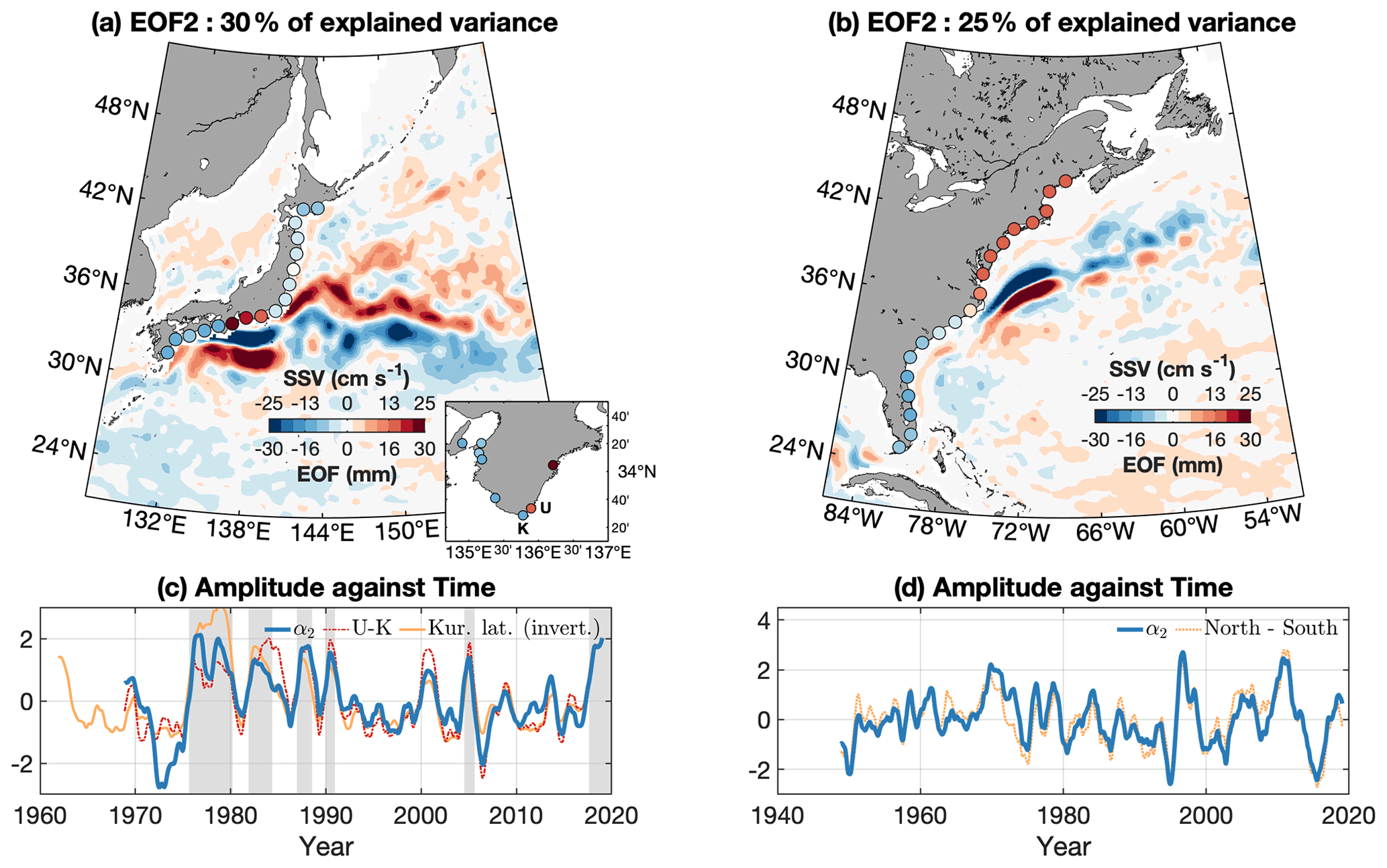
Figure 6The second EOF (ϕ2) of the gridded tide-gauge-based sea-level anomaly (circular markers) from the Pacific (a) and the Atlantic (b). The associated principal components α2 are shown as thick dark blue lines for the Pacific (c) and Atlantic (d). Also in (c), the Kuroshio southernmost latitude south of Tōkai is represented by the solid orange line (positive values indicate Kuroshio further to the south); the difference between sea level at Uragami and Kushimoto is represented by the dot-dashed red line, and grey shading represents periods of typical large meander (JMA, 2018). In (d), the dashed yellow line is the sea-level difference between the averages of northern and southern groupings of tide gauges, as in McCarthy et al. (2015). All time series in (c) and (d) are normalized. For each basin, colour shading in (a) and (b) is the sea surface velocity magnitude composite difference based on the principal component α2 (period of minus period of ). The arbitrary threshold of was used, but taking any number between 0 and 1 leads to similar patterns. The inset in (a) presents the regression coefficient obtained when the principal component is regressed on the original tide gauges, with a zoom-in on the Kii peninsula.
In the Pacific, a second group west of Kii varies in antiphase with the Tōkai gauges, with ϕ2 on average equal to −1.2 cm. In the Atlantic, ϕ2 south of Cape Hatteras is on average −0.8 cm (Fig. 6a). In both cases, the magnitudes of these negative variations are more than 2 times smaller than the magnitude of the positive variations (north of Cape Hatteras and south of Tōkai).
In the Pacific, large amplitudes in the EOF ϕ2 are confined upstream of the Kuroshio separation point, whereas the Atlantic mode is dominated by the variability past the separation point to the north. Furthermore, the velocity composite difference based on α2 and obtained in a similar manner presents very different patterns from one basin to another (colour shadings, Fig. 6a and b), which we return to in more detail below. As the two modes are different, we discuss them separately.
3.2.3 The second mode in the Pacific
The principal component α2 obtained with the Pacific gauges is closely linked with the typical large meander of the Kuroshio. Negative values coincide with known periods when the Kuroshio took the tLM pathway (as acknowledged by the Japan Meteorological Agency – JMA, 2018: August 1975 to March 1980, November 1981 to May 1984, December 1986 to July 1988, December 1989 to December 1990, July 2004 to August 2005, August 2017–2020; see shading in Fig. 6c), whereas the Kuroshio took one of the NLM pathways the rest of the time or, less often, an atypical path.
The principal component is extremely close (r=0.83, significance well above 99 %) to the difference in sea level between Kushimoto and Uragami (thin dot-dashed red line in Fig. 6c), two stations located either side of Cape Shiono-Misaki on the Kii peninsula, which is the point of separation between the two groups of coherent variability highlighted in the previous section. The relationship between the tLM periods and the sea-level difference between those two stations has been known since the early work of Moriyasu (1958, 1961) and was investigated by Kawabe (1985, 1995, 2005), among others. The inset in Fig. 6a presents the regression coefficient obtained when the principal component is regressed on the original tide gauge records, with a zoom-in on the Kii peninsula. Despite geographical proximity (less than 20 km), the stations of Kushimoto and Uragami (indicated by a K and a U in the inset) are affected very differently by the second mode. The amplitude at Uragami is negative and is positive at Kushimoto. On the other hand, as was discussed previously, the leading EOF is of same sign and relatively similar magnitude on all of the southern coast of Japan (see the inset of Fig. 5a for the amplitude of the leading mode at Kushimoto and Uragami), and the other modes have negligible amplitudes in the region. From there, subtracting the Kushimoto time series from the ones from Uragami essentially gets rid of the influence of the leading EOF and reveals the underlying variability south of Tōkai.
The Japan Meteorological Agency estimate of the southernmost latitude of the Kuroshio axis south of Tōkai (136–140∘ E) is shown in Fig. 6c (orange line, axis is inverted so that southern shift is a positive anomaly). Correlation with the principal component α2 is strong and highly significant (r=0.82, significance >99 %), confirming that the mode is a footprint of the large meander. Note that the correlation is slightly higher with the principal component than with the difference between Kushimoto and Uragami (r=0.78, significance >99 %).
The velocity composite, derived on high () minus low () values of α2 as was done for the leading modes, is shown in Fig. 6a. When the principal component is strongly positive, i.e. when the Tōkai coastal sea level is high, the Kuroshio south of Tōkai (135–141∘ E) is found farther south than when the principal component is negative, in which case it is found much closer to the coast. The positive velocity patch intersects the negative velocity patch so that the Kuroshio path east of the Bōsō peninsula is closer to the coast during the positive α2 periods and flows northeastward, whereas during the negative period, the Kuroshio essentially flows eastward. Simply put, the negative velocity pattern represents the non-large meander paths, and the positive velocity pattern represents the large meander paths (see Fig. 1). The situation east of the ridge (>140∘ E) is roughly similar to Fig. 5a; that is, the Kuroshio Extension is found more to the north when the principal component is positive. The negative velocities are also more scattered than their positive counterparts, highlighting the fact that the KE was more stable during the period of positive α2 (see also Sugimoto and Hanawa, 2012).
3.2.4 The second mode in the Atlantic
The principal component associated with the second EOF in the Atlantic increases from 1948 to the early 1970s, followed by a decrease until the mid-1990s, with inter-annual deviations from those long-term changes (Fig. 6d). The mid-1990s mark an abrupt change, with the inter-annual variability increasing greatly in amplitude from then onwards. This is shown in Fig. 7a, which presents the moving standard deviation of α2 obtained with a 15-year running window (solid blue line).
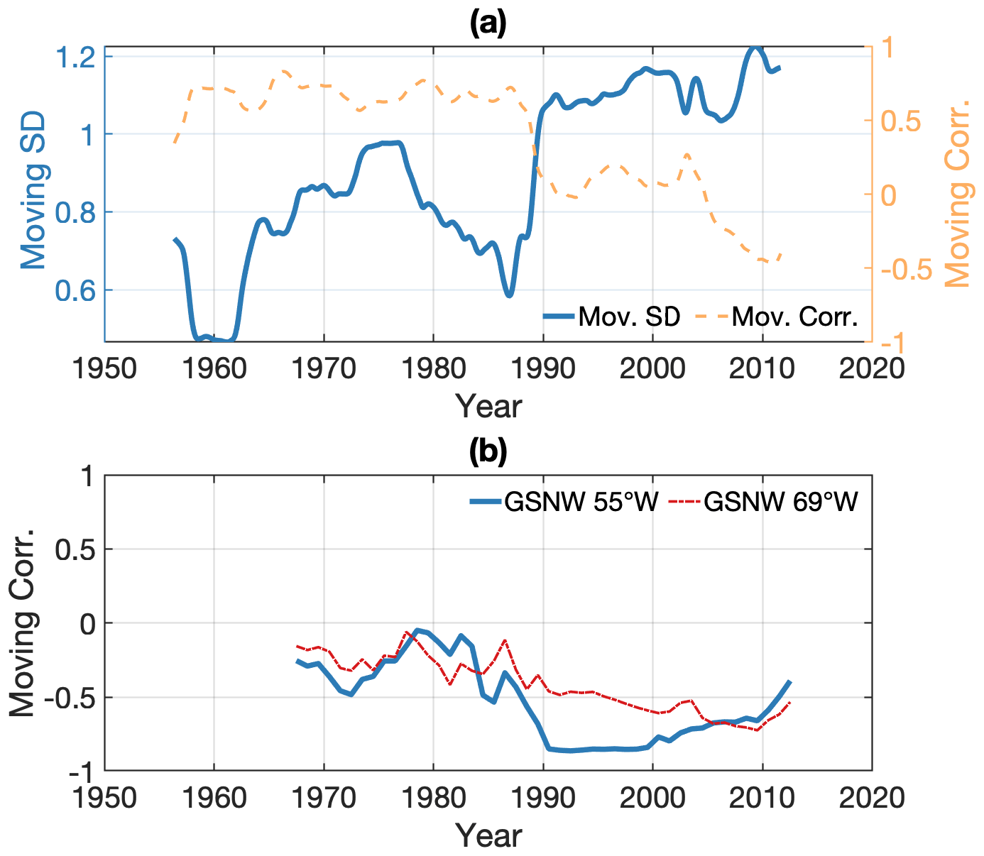
Figure 7(a) Moving standard deviation of α2 with a 15-year running window (solid blue line) and moving correlation with the same windowing between the northern and southern Atlantic gauge grouping averages (orange dashed line). The latter is the same as the blue line in Fig. 4a. (b) Moving correlation with a 15-year running window between the second principal component α2 and our GSNW index (solid blue line) and between α2 and our GSNW index computed on 75–69∘ W (dot-dashed red line).
As noted by Valle-Levinson et al. (2017), the variability of this mode has already been shown in the past by the difference in the sea level either side of Cape Hatteras (McCarthy et al., 2015; Woodworth et al., 2017). The yellow dashed line in Fig. 6d shows the difference between the averages of northern and southern gauge groupings. In comparison with the mean sea-level difference indices of McCarthy et al. (2015) and Woodworth et al. (2017), the time series are flipped, as we computed the difference as north minus south rather than the other way around. The agreement between the sea-level difference and α2 is very high, r=0.88 (significant above 99 %). As for the difference between Kushimoto and Uragami, subtracting the sea level south of Cape Hatteras from north of Cape Hatteras (or reversely) minimizes the influence of the leading mode. Indeed, the difference between ϕ1 magnitude either side of Cape Hatteras is 1.3 cm on average, whereas the difference between the EOF ϕ2 magnitude either side of Cape Hatteras is 2.5 cm.
The velocity composite exhibits two well-defined patterns of opposite sign off Cape Hatteras, indicating that the positive (negative) phases of α2 are concurrent with a southern (northern) shift of the Gulf Stream west of 69∘ W (Fig. 6b). The patterns bear some resemblance to the ones obtained with α1 presented in Fig. 5b, but the amplitudes of the composite along the Gulf Stream Extension make a strong contrast. The positive and negative velocity patches are now maximum in the region west of 69∘ W, where they have greater across-shore width than the ones obtained with α1 (Fig. 5b). There, because the −25 to 25 cm s−1 colour scale was retained for comparison with the other modes, the composite amplitudes are largely clipped. They are in the range of (±)40–60 cm s−1, larger than the magnitudes obtained with α1 in the same region, which were in the range of (±)10–40 cm s−1. On the other hand, composite amplitudes east of 69∘ W are smaller when obtained with α2 than when obtained with α1. In this second region, the α2-based composite is also less consistent, with the negative velocities intruding southward and splitting the positive pattern in two at ∼68∘ W. Hence, the link between α2 and the Gulf Stream Extension meridional shifts in this second region is not as clear as the one obtained with α1.
EOF analysis showed similar features of the leading mode of the two basins. The leading mode explained 47 % of the variance in the Pacific gauges and 60 % of the variability in the Atlantic gauges. Their spatial patterns were similar, having a greater amplitude south of the separation points than to the north (Fig. 5). In both basins, the temporal amplitudes of these similar modes were shown to co-vary with the meridional shifts of the western boundary current extension.
An important dissimilarity, however, is that the amplitude of the leading EOF in the Atlantic decreases gently north of the separation point, while the transition is abrupt in the Pacific. This result contrasts with the findings of Valle-Levinson et al. (2017), who obtained a leading EOF of the Atlantic gauge records with a less marked northward decrease in amplitude. Although the different starting and ending periods may play a role, we find that this discrepancy mostly arises because of the correction we applied for surge-driven sea-level change (Appendix A). This result, however, should not be interpreted as a demonstration that the atmosphere plays a role in extending the southern variability northward. Rather, the surge correction reduces the variance north of Cape Hatteras, which better constrains the EOF analysis and reduces undesired compensation between modes.
When the EOF analysis is recalculated restricting the period to 1960–1990, when greater coherence either side of Cape Hatteras is seen (Fig. 4b), the northward decrease in ϕ1 is still apparent. This is an important result because previous studies had excluded the Gulf Stream and its extension as plausible drivers of the sea level on the western coast of the North Atlantic basin on the basis that such drivers were not able to explain coherence across Cape Hatteras (Thompson and Mitchum, 2014; Valle-Levinson et al., 2017). On the contrary, we found that the Gulf Stream separation marks the point from which the mode's imprint of sea level diminishes, suggesting that the Gulf Stream presence is a plausible sea-level driver – in line with other studies (e.g. Ezer, 2015; Ezer et al., 2013; Ezer, 2019). In our view, the northward decrease in ϕ1 is related to the orientation of the Gulf Stream Extension, which gradually moves away from the shoreline north of 35∘ N. Following the same idea, the difference between the abrupt decrease in the EOF amplitude in the Pacific and the gradual decrease in the Atlantic arises from the different WBC extension orientations, with the Gulf Stream Extension flowing northeastward and the Kuroshio Extension eastward.
The leading mode temporal amplitudes in both basins are in agreement with the location of the WBC extensions in both altimetry-derived sea surface velocities and in situ subsurface temperature. In the Pacific, anomalous wind stress curl triggers westward-propagating baroclinic jet-trapped Rossby waves that shift the jet meridionally (Sasaki et al., 2013; Sasaki and Schneider, 2011a; Sugimoto and Hanawa, 2009; Ceballos et al., 2009). A similar mechanism has been proposed for the Atlantic (Sasaki and Schneider, 2011b; Sirven et al., 2015). Sasaki et al. (2014) hypothesized that the incoming jet-trapped Rossby waves, which are responsible for the extensions' shifts, break on the western boundary and propagate equatorwards as Kelvin or other coastally trapped waves, linking the extension variability to coastal sea level. Because the long jet-trapped Rossby waves provide a mass input to the western boundary, which has a narrower meridional extent than traditional Rossby waves, the alongshore coastal sea-level gradient is maximum near the WBC separation point (Equation 1). This leads to a “shadow” coastal area north of the separation point, which is less affected by the incoming jet-trapped wave, and an “active” area, which sees the progression of the coastal wave (Sasaki et al., 2014), explaining the EOF patterns in Fig. 5. Hence, although Sasaki et al. (2014) focused on the KE and southern Japan sea level, our results support the idea that such a mechanism could explain the link between the coastal sea level and the extension meridional location observed in both oceans. It is true that we found that, in the Atlantic, the correlation between the GSNW and the leading principal component of the sea-level variability is maximum when the GSNW lags by about 1 year, but we must emphasize that we found significant correlation between the GSNW and the Atlantic α1 at zero lag, in agreement with a mechanism of coastal waves following the jet undulation.
The SSV analysis showed difference between the two basins in the upstream velocity patterns associated with α1. The upstream Kuroshio was displaced on-shoreward south of Tōkai, but the Gulf Stream south of Cape Hatteras moved off-shoreward during the positive phase of α1 (Fig. 5a and b). The two situations are not necessarily opposing, as off-shoreward motion is also seen southeast of Kyūshū in the Pacific (around 30∘ N, 132∘ E; see Fig. 5a). So, when α1 is positive, the Kuroshio shifts off-shoreward south of Tōkai, but moves in-shoreward southeast of Kyūshū. Nonetheless, the patterns in the two basins are visually quite different. These patterns may suggest that some mechanisms more involved than a pure Kelvin wave (Sasaki et al., 2014) are at work. The velocity patterns seen south of Japan relate to the alternation of offshore NLM and nearshore NLM paths. Unfortunately, with the data at our disposal we cannot assess whether the upstream velocity patterns associated with α1 extend before the satellite era as we did for the downstream variability with the GSNW and KEI indices – although it should be noted that Kawabe (1989) showed the same agreement between the sea level south of Japan and alternation of offshore NLM and nearshore NLM for the period 1964 to 1975. Interestingly, transition from one of these paths to the other is related to the Kuroshio transport but the established paths are not (Kawabe, 1989, 1990), meaning that differences in coastal sea level between oNLM and nNLM seen in α1 are not due to geostrophic adjustment. The proximity (remoteness) of the warm water of the Kuroshio during nNLM (oNLM) might be responsible for the sea-level rise (drop) through thermosteric adjustment (Kuroda et al., 2010; Kawabe, 1989). A mechanism linking the upstream sea level to the water temperature in the vicinity of the Gulf Stream has also been proposed (Domingues et al., 2018), although this does not explain why the Gulf Stream was shifted in-shoreward when the Kuroshio was shifted off-shoreward.
The EOF analysis highlighted very different second modes in the two basins. The second EOF explained 30 % of the variance in the Pacific gauges and 25 % of the variability in the Atlantic gauges. In the Pacific, this second mode is the manifestation of the meandering of the Kuroshio upstream of its separation point, whereas the second EOF in the Atlantic is mainly associated with variability north of Cape Hatteras, the separation point.
In the Pacific, the typical large meander influence on the sea level south of Tōkai was shown in our analysis and has been known for many decades (Moriyasu, 1958, 1961; Kawabe, 1985, 1995, 2005). The elevated values of α2 closely match the typical large meander periods (Fig. 6c), with the exception of April 2000–April 2001 when α2 was high despite the Kuroshio not being in a tLM phase. Sugimoto et al. (2019) highlighted the fact that, during tLM phases, the strengthening of the anticyclonic circulation accelerates a westward coastal current in the 137–140∘ E region, which allows the intrusion of warm Kuroshio water south of Tōkai. Between 2000 and 2001, this westward flow, which closes the anticyclonic circulation south of Tōkai, can also be observed. It is clearly apparent in monthly snapshots (Fig. S3 in the Supplement) and in the mean velocity between April 2000 and April 2001, although to a lesser extent (Fig. S4b in the Supplement). SST and SSH averages over this period show that the intrusion of warm water south of Tōkai goes along with a rise of the SSH there, as do composites obtained over tLM periods (Fig. S4c–f in the Supplement). In fact, the major distinction from the tLM period is that between 2000 and 2001, the Kuroshio veered northward east of the ridge (or on the ridge at 140∘ E). These types of pathways are sometimes called straddling large meanders because, in contrast to typical large meanders, the anticyclonic eddy straddles the Izu–Ogasawara Ridge at 140∘ E.
The common denominator to the tLM and such atypical paths is the presence of the westward flow identified by Sugimoto et al. (2019), which brings warm waters south of Tōkai. We hypothesize that the sea-level rise recorded by the gauges in the region is forced by the intrusion of the Kuroshio warm water brought by such currents (geostrophic tilting and/or steric rise). From a coastal sea-level perspective, there is no qualitative difference between the forcing of a typical large meander and the forcing of atypical paths that straddle the ridge.
The second mode of variability of the Atlantic tide gauge is perhaps the most puzzling mode among the four modes discussed here. As was indicated by Valle-Levinson et al. (2017), differentiating north minus south of Cape Hatteras sea level approximates this mode well (McCarthy et al., 2015; Woodworth et al., 2017). However, the EOF ϕ2 has a much greater absolute magnitude north of Cape Hatteras than south, in contrast to Valle-Levinson et al. (2017). This indicates that simultaneous anti-variations south of Cape Hatteras are weak. Again, this difference arises because of the correction we applied to remove local atmospherically driven variability. It suggests that, at first order and for the period 1948–2019, differentiating the sea level across Cape Hatteras removes the influence of the leading mode on the sea-level variability north of Cape Hatteras. In this region, ϕ1 and ϕ2 have comparable amplitudes, despite the northward decrease in the strength of the leading mode.
Our results indicate a clear change in the variance of α2 occurring around ∼1990 (Fig. 7a). Previous studies showed an increase in the agreement between the North Atlantic Oscillation and the sea-level variations north of Cape Hatteras occurring around the same time (Andres et al., 2013; Kenigson et al., 2018). Studies that focused on the low-frequency (7-year filtered) mean sea-level difference across Cape Hatteras (McCarthy et al., 2015; Woodworth et al., 2017) noted greater agreement with the NAO since the second half of the 20th century than before. For example, Woodworth et al. (2017) report a correlation of −0.62 for the period 1950–2014 between the difference of New York minus Key West and the NAO, as well as a lower correlation of 0.21 for the period 1913–1949. It is reasonable to believe that the strong agreement since ∼1990 contributes to the overall low-frequency agreement since 1950, in conjunction with anticorrelated multidecadal variability: sea-level rise north of Cape Hatteras (NAO decline) between 1948 and ∼1970 as well as between ∼1990 and ∼2010 and sea-level drop (NAO increase) between ∼1970 and ∼1990.
Our analysis based on sea surface velocity composites highlighted the agreement of α2 with the Gulf Stream Extension meridional location west of 69∘ W, consistent with Andres et al. (2013). The relevance of satellite measurements for interpretation of ocean dynamics prior to ∼1990 is, however, questionable. The sharp increase in the variance of the mode around ∼1990 raises the issue of whether this mode represents the pursuance of the same physical phenomenon throughout the whole period of 1948–2019 or if a mechanism supplanted another around ∼1990. We find that α2 has a non-stationary relationship with the GSNW index in this study (Fig. 7b, solid blue line). The correlation between the GSNW and α2 is −0.45 (significant above 99 %) over the full period of 1948–2019, quite similar to the correlation between the GSNW and α1, but this agreement is due to the period after ∼1990 when correlation is (>99 %), while the correlation between 1948 and 1989 is −0.17 (61 %). Hence, the relationship with the location of the Gulf Stream is largely limited to the recent era, which complicates understanding of the forcing prior to α2 variance change around 1990. Note that here we use 1990 as a change point for simplicity, but similar results are obtained when using 1987 (Kenigson et al., 2018; Boon, 2012) or 1994, which corresponds to the first strong negative α2 dip after more than 40 years.
One mechanism in particular is hypothesized to have tied the Gulf Stream location west of 69∘ W and the Nova Scotia to Cape Hatteras sea level together since ∼1990: Andres et al. (2013) argued that the coastal sea level is proportional to the geostrophic southward shelf transport, which interacts with the Gulf Stream at the separation point at which the shelf transport and the Gulf Stream meet. The use of the inshore sea level alone to diagnose the shelf transport is supported by a variance minimum in SSH anomaly located on the shelf break. Whether the Gulf Stream dictates the shelf sea level – and hence the shelf southward transport – or the other way around is an open debate (Andres et al., 2013; Ezer et al., 2013; Peña-Molino and Joyce, 2008).
Andres et al. (2013) hypothesized that the shelf transport is triggered by the alongshore wind forcing over the shelf and eventually drives the movements of the Gulf Stream to the south, rather than the opposite. A strong negative correlation between the coastal sea level north of Cape Hatteras and the alongshore wind stress over the northern part of the shelf supported the hypothesis. Kenigson et al. (2018) highlighted the fact that the year 1987 marked an abrupt change in the wind orientation above the US northeast coast and Canadian east coast. If this hypothesis is indeed correct, it is intriguing that such sea-level variability appears in our analysis given that the tide gauge records have been corrected for instantaneous wind forcing, especially as the sea-level response to the atmospheric forcing that was removed from the record (Appendix A) is quite different from α2 (Fig. S8b in the Supplement). To investigate the question, we repeated the procedure of Andres et al. (2013) and correlated the principal component against the detrended NCEP wind stress fields projected onto a 20∘ from zonal angle, roughly corresponding to the orientation of the shelf. A 19-month filter was applied to the wind stress for compatibility with the principal component. Figure S5a in the Supplement presents the correlation over the full period of 1948–2019 between α2 and the along-20∘ wind stress. The correlation above the shelf does not exceed 0.23. When the correlation is computed reducing the period to 1990 onwards, the patterns are greatly changed (Fig. S5c in the Supplement), as noted by Andres et al. (2013) and Kenigson et al. (2018). In contrast to Andres et al. (2013), however, the negative correlation pattern in Fig. S5c is shifted towards the Gulf of Saint Lawrence and east of Newfoundland so that the agreement with the alongshore wind on the shelf remains negligible everywhere. Hence, the variability of α2 is not due to the alongshore wind stress above the shelf, and we can say that the latter has been successfully removed from the tide gauge records by our correction for local atmospheric forcing. Furthermore, the role of remote wind stress in the Gulf of Saint Lawrence or east of Newfoundland is uncertain as well because at these latitudes the NAO is a confounding variable. When corrected for the NAO, the correlation between the alongshore wind stress and α2 is not significant anywhere on sea (Fig. S5d in the Supplement). This does not necessarily exclude alongshore wind stress in the Gulf of Saint Lawrence or east of Newfoundland as a possible driver of the variability of α2 since 1990, but it indicates that any other forcing strongly correlated with the NAO is as likely to be a driver.
Alternatively, density anomalies formed in the Labrador Sea propagating southward along the western boundary, either as coastally trapped waves or advected within the deep western boundary current, have been proposed as drivers of the sea-level variability north of Cape Hatteras (Frederikse et al., 2017). However, existing indices of the AMOC and DWBC do not show the same variability as α2 (Caesar et al., 2018; Thornalley et al., 2018). Finally, we have not considered the role of salt (or lack of) and water volume input to the shelf caused by both river discharges and eddies detaching from the Gulf Stream, which are an additional potential driver of the sea level on the shelf (Piecuch et al., 2018).
EOF analysis can help us to understand the major distinctions observed in the alongshore sea-level coherence between the two basins. Upstream of the separation point in the Pacific, the cross-correlation analysis highlighted two distinct groupings either side of the Kii peninsula. This is the point at which the Kuroshio path either follows the large meander or stays close to the coast on a non-large meander path (Fig. 1). The EOF analysis revealed that the sea level in the region east of Kii is the sum of the two leading modes, whereas in the region west of Kii the sea level is well approximated by the first mode only; the first mode is associated with the Kuroshio Extension meridional motions and the following mode with meandering south of Japan. Hence, the second grouping of co-variability south of Japan is due to the emergence of (a)typical large meanders, which are an additional forcing for the sea level east of Kii. This forcing has no equivalent in the Atlantic, and therefore there is only one distinct grouping of variability south of Cape Hatteras.
In the Atlantic, the moving correlation analysis showed that the agreement between gauges south and north of Cape Hatteras changed strongly around This is an additional distinction between the Atlantic and Pacific, as no coherence change of such magnitude was observed between the Oyashio and west of Kii groupings in the Pacific. Figure 7a presents the moving correlation between the southern and northern gauge averages (dashed orange line) alongside the standard deviation of the principal component α2 computed with a moving 15-year window (solid blue line). It is apparent that the change in variance of α2 is concurrent with the shift in correlation between north and south of Cape Hatteras seen in the moving correlation analysis. The EOF analysis hence leads us to interpret the change in coherence across Cape Hatteras as due to an increase in the variability north of Cape Hatteras appearing in the second mode. Clearly, this is a realistic possibility, but a caveat should also be stated. As previously mentioned, we were not able to link this second mode to a continuous physical mechanism, with agreement of α2 with both the Gulf Stream position and with the winds seen only after the increase in the mode variance (Figs. 7b and S5 in the Supplement). It is thus possible that this EOF–PC couple is solely statistical and cannot be understood as a continuous physical mode. If a physical process replaced another around 1990, for example under the background influence of Gulf Stream transport changes or AMOC changes, it is possible that EOF analysis would not distinguish between the two mechanisms and mix them into a single statistical mode. That is because EOF analysis is not designed to deal with physical mechanisms whose spatial footprints are non-stationary in time (such as disappearing or emerging modes).
This study presents a consistent analysis of the two western boundary regions in the northern Atlantic and northern Pacific. The agreement between the upstream sea-level variability and the WBC extensions' meridional shifts was highlighted in the two basins conjointly. In both oceans, this relationship was previously observed for the altimetry period (Sasaki et al., 2014; Ezer, 2019), but here we show that it holds for the longer periods of 1948–2019 for the Atlantic and 1968–2019 for the Pacific. This agreement, shown for both basins, supports the mechanism of Sasaki et al. (2014) of trapped Rossby waves propagating within the western boundary current extensions, shifting them meridionally en route and progressing into coastally trapped waves at arrival at the coast, consequently modifying the inshore sea level. The state-of-the-art wave theory of Sasaki et al. (2014) is elegant, but there are some limitations that we believe are useful to point out for future developments in the relationship between western boundary current extensions and upstream sea levels. First, the upstream sea level is known to co-vary with the upstream bottom temperatures at the shelf break and on the shelf (Kuroda et al., 2010), as well as with temperature within the western boundary current vicinity (Domingues et al., 2018). This weakens the Sasaki et al. (2014) hypothesis or at least limits the spectrum of possible coastally trapped waves to waves with non-zero cross-shore flow, which are able to drive warm water on and off the shelf (e.g. topographic Rossby waves). Secondly, the role played by the path variability upstream of the separation point is unclear. In the Pacific, the upstream patterns of velocity in Fig. 5a feature the offshore and nearshore non-large meander paths (Fig. 1), which have not previously been understood as propagating coastally trapped waves. Furthermore, positive (negative) α1 values were shown to be concurrent to inshore (offshore) paths south of Japan, whereas south of Cape Hatteras, the opposite was observed (positive α1 associated with an offshore path). If coastally trapped waves indeed drive the upstream coastal sea level, it is conceivable that they also cause the concurrent offshore (inshore) shifts of the western boundary currents upstream of their separation point. Yet, it is unclear why they would drive opposite behaviour in term of paths in the two basins. Finally, recent studies have also linked the inshore upstream sea level with the subtropical gyre interior sea surface height and/or temperature (Woodworth et al., 2014; Thompson and Mitchum, 2014; Volkov et al., 2019; Ezer, 2019). These diverging views underscore the difficulties of understanding the causal relationship between the WBC extension and the upstream sea level. In the Atlantic, our finding that the upstream sea level is in agreement with the Gulf Stream Extension's position converges with the very recent study of Dangendorf et al. (2021), which showed that the stero-dynamic portion of the upstream tide gauge variability was correlated with the steric height signal in the Gulf Stream Extension. The results of the present study and of the recent work of Dangendorf et al. (2021) and Ezer (2019), all presenting linkages between the Gulf Stream Extension and the upstream sea-level variability, are hence important and novel contributions to the understanding of Gulf Stream dynamics. Further work is required to precisely comprehend the mechanisms that link the upstream sea level and the western boundary current extensions' variability.
We showed that dissimilarities between Japanese and American inshore sea level emerge in the second mode of variability. In the Pacific this relates to upstream mesoscale dynamics (Kuroshio large meander), whereas in the Atlantic, the second mode is mainly associated with changes north of Cape Hatteras, the separation point of the Gulf Stream, although weak anti-variations exist to the south. In the Pacific and in comparison with existing studies, we noted that the sea level south of Tōkai was affected by the presence of large meanders in a broader sense, including atypical meanderings that straddle the Izu–Ogasawara Ridge. In the Atlantic, EOF analysis highlighted the fact that the variability of the second mode drives the coherence across Cape Hatteras. However, it is not clear whether a physical mechanism – well represented by the second mode of EOF analysis and with increasing effects after ∼1990 – caused the disconnect north and south of Cape Hatteras or if a new process appeared circa 1990, which cannot be resolved by stationary EOF analysis. We showed that the strong link of this statistical mode with the shifts of the Gulf Stream Extension west of 69∘ W is relatively recent and does not extend prior to We also showed that the local alongshore wind was an unlikely driver of this mode variability. Hence, whether this Atlantic second mode represents the pursuance of the same physical phenomenon or if a mechanism supplanted another around ∼1990 is still an open question.
Because the tide gauge networks in both oceans extend further back in time than the period analysed in this study, inshore sea level has potential for reconstruction of the variability of the ocean circulation mode of variability. Reconstruction of past large meander events requires at least two gauges either side of the Cape Shiono-Misaki on the Kii peninsula; traditionally, the tide gauges of Uragami and Kushimoto are used. The two stations are respectively available from 1965 and 1957 in the PSMSL revised local reference (RLR) catalogue. Using sea-level aggregates based on the correlation groupings (Fig. 3) rather than the two individual tide gauge records, in a manner akin to McCarthy et al. (2015), allows the extension of the analysis up to 1944 and characterizes 1953–1955 and 1959–1963 as large meander periods, similar to Moriyasu (1958, 1961) and Kawabe (1985, 1995, 2005). On the other hand, further understanding of the forcing on sea level prior to ∼1990 is needed to use the north of Cape Hatteras gauge records as a proxy for ocean and/or atmosphere variability prior to that date.
Finally, although the causal link between the upstream sea level and the meridional shifts of WBC extensions is not yet completely understood, our results suggest that upstream inshore tide gauges, such as Key West (available from 1913 in the PSMSL RLR database), Fernandina Beach (1897) or Hosojima (1930), could be used as proxies for the extension meridional shifts and, by extension, the forcing responsible for such meridional shifts. In the Pacific, tide gauges in the region west of Kii, where the sea level is less affected during large meander periods, should be preferred. That tide gauges can be used to infer past open-ocean dynamics is a result in line with some recent studies which have reconstructed open-ocean sea level (and hence ocean dynamics) using the global tide gauge network and advanced statistical methods (Ezer and Dangendorf, 2020; Dangendorf et al., 2019, 2021).
Following the work of Dangendorf et al. (2013, 2014), Frederikse et al. (2017), and Piecuch et al. (2019), we compute the inverse barometer and wind-surge contributions to sea level using multiple linear regression, with pressure (p) as well as alongshore (τ∥) and across-shore (τ⊥) wind stress anomalies interpolated at each tide gauge location as predictors. The angles used for the rotation in across-shore and alongshore coordinates are presented in Tables S1 and S2 in the Supplement. The quality of a regression primarily depends on the correlation between the explanatory variables and the period width. Here, the pressure and winds are not independent. Hence, for each tide gauge, an “all-possible” regression procedure was designed. This means that the model with the three regressors is tested (Eq. A1), alongside all the possible models for which the first, second and (or) third term of the equation are (is) ruled out. In total, combinations of possible regressions are tested at each tide gauge.
The regressions return the regression coefficients β1, β2 and β3 that describe the relationship between pressure, alongshore and across-shore winds, and the gauge record. 𝒪(t) represents the unexplained residual. Y intercepts are estimated to improve the computation, but are not removed to form the residual 𝒪(t). Note that the inverse barometer effect is not proportional to the local pressure alone but to the difference between the local pressure and the global sea-level pressure averaged over the oceans. Also, β1 is preceded by a minus (−) because a rise of local atmospheric pressure makes sea-level fall and vice versa.
To determine the best model for each tide gauge, 95 % confidence intervals are computed for each regression coefficient within the MATLAB built-in function. The regression models that feature one (or several) coefficient confidence interval(s) crossing zero are excluded. Then, the best regression is defined as the one with the highest adjusted coefficient of determination , which is the proportion of the variance in the gauge record that is predictable from the atmospheric predictors, adjusted for their number (see Eq. A2):
where m is the number of time steps, nr is the number of regressors for that particular model () and the sum of the obtained atmospheric contributions.
Figure S6a and b in the Supplement respectively present the regression coefficients β1, β2 and β3 as well as their 95 % confidence interval for the Atlantic and for the Pacific gauges. For each gauge, only the output of the best regressions is shown. Hence, the number of regressors is not always three, in particular for the Japanese stations. The adjusted coefficients of determination (bottom) for each tide gauge are shown in Fig. S7 in the Supplement.
We compute values for β1 of 0.11 and 0.9 mm Pa−1 on average for American and Japanese gauges, respectively (see the green line in Fig. S6a and b in the Supplement). In both regions, the computed β1 values are comparable to the theoretical mm Pa−1 expected for an inverse barometer response (dashed green line). The pressure is always one of the explanatory variables of the best regression, highlighting the importance of the inverse barometer effect on sea level. Across-shore coefficients are high in locations upstream of the estuaries of Delaware Bay and Chesapeake Bay (TGs 7, 8, 9, 10 and 12: Washington DC, Solomons Island, Annapolis, Baltimore and Philadelphia). There, the wind setup is amplified by the funnelling effect of the estuaries. The nearby stations of Sewells Point (TG 6) and Lewes (12) are, in contrast, much less affected because they are located at the mouth of the estuaries. The best regression does not feature the across-shore wind north of Cape Cod (TG 20–22). The obtained alongshore coefficients show less deviation from the average of −7.9 m3 N−1, yet the maximums are also found in the estuary region. North of Cape Cod (TG 14 to 23), we obtain values for β2 an order of magnitude greater than reported by Piecuch et al. (2019). For most of the Japanese gauges, the best regression does not feature either the across-shore or the alongshore component of the wind stress, as using all of the explanatory variables does not explain more variability in the tide gauge records. However, a consistent effect of the alongshore winds for the southern tide gauges (TGs 1–2 and 4–19) is revealed by the regression.
Figure S7 in the Supplement presents the adjusted coefficient of determination (Eq. A2). It better depicts the effect of the atmosphere on the sea level than the regression coefficients alone, as even a weak βi coefficient could greatly affect the sea level if the corresponding regressor variability is important at the tide gauge location. Consistently with Piecuch and Ponte (2015), we find that the atmospheric effect on sea level explains an important part of the gauge variability north of Cape Hatteras (Fig. S7a in the Supplement), with on average higher than 40 %. This result is in agreement with Piecuch et al. (2019), who reported a value of 39 %, although their analysis focussed on the period 2004–2017. In contrast, only 20 % of the variability in the time series of the southern gauges can be explained with the regression, with some deviations from that mean. This is consistent with previous findings of Woodworth et al. (2014), and we observe a similar pattern in the Pacific. The tide gauges located north of the Bōsō peninsula (Fig. S7b in the Supplement) show high , whereas tide gauges south of Japan (TGs 1 to 24) are not at all explained by the atmospheric forcing. The drop in the variability explained by the atmosphere is located at the separation point of the western boundary current in both regions (Cape Hatteras and the Bōsō peninsula). This does not necessarily means that there is no atmosphere-related sea-level change south of the separation points but rather that they are dwarfed by other sources of variability.
Figure S8a and b in the Supplement present the mean ζAtm north of the Bōsō peninsula and Cape Hatteras, respectively, where ζAtm is the sea level driven by the atmosphere and regroups the first three terms of Eq. (A1) (). It is apparent that, while most of the variability is intra-annual, there is also inter-annual variation.
In the paper, we consider the residual 𝒪(t) (Eq. A1), which represents the sea-level variability unexplained by the atmospheric variables, to be the sea level “corrected” from the local atmospheric forcing and refer to it as ζ for simplicity.
Here we provide further insights on the empirical orthogonal function (EOF) analysis used to objectively reduce the sea-level anomalies in an ensemble of modes.
EOF decomposition using a covariance matrix is performed on tide gauge records after they are interpolated on a regular grid to prevent variability in better-sampled regions from being favoured in the analysis. First, tide gauges located in the Chesapeake Bay and the Inland Sea (west and east separately) are averaged and associated with a virtual location at the mouth of the Chesapeake Bay, the Bungo Channel and the Kii Channel, respectively. Then, in the Pacific (Atlantic), the 20 (18) remaining gauge records plus the two (one) aggregated estuary records are interpolated onto a regular alongshore grid with 150 km spacing.
The modes are composed of a time-varying coefficient α, the principal component (PC) and an associated spatial-varying coefficient ϕ, the empirical orthogonal vector or function (EOF):
where represents the modes, which are ordered by decreasing percentages of total variability explained, n is the total number of spatial grid points, and x and t are space (alongshore) and time, respectively.
Note that the spatial amplitudes ϕ that are discussed within the text are relative to periods when their associated principal components α are equal to the standard deviation: that is, αi=1. For example, it is shown that the amplitude of the leading mode south of Japan, ϕ1, is on average 2.3 cm (Fig. 5a). The peak-to-peak amplitude of the associated temporal amplitude α1, defined as the difference between the maxima of late 2004 and the minimum of 1985, is roughly equal to 5 (Fig. 5c). Hence, between 1985 and 2004, the sea-level rise associated with this mode is ∼12 cm south of Japan.
GSNW and KE indices from this study are available online, as are the principal components α1 and α2. They can be downloaded in “.csv” spreadsheet format at https://doi.org/10.5281/zenodo.4659318 (Diabaté et al., 2021). When using these time series, please cite the present study appropriately. The GSNW and KE indices are derived from the EN4 quality-controlled ocean temperature profiles (Good et al., 2013, EN4.2.1) available at https://www.metoffice.gov.uk/hadobs/en4/ (last access: 2 June 2021) and from the 1981–2010 objectively analysed mean temperature of the World Ocean Atlas 2018 (Locarnini et al., 2018, WOA18) available at https://www.nodc.noaa.gov/OC5/woa18/ (last access: 28 September 2021). Underlying datasets for α1 and α2 include (1) the original monthly tide gauge data available from the Permanent Service for Mean Sea Level (PSMSL, https://www.psmsl.org/, last access: 18 October 2021), (2) sea-level pressure and 10 wind speeds from the NCEP/NCAR Reanalysis 1 (Kalnay et al., 1996) distributed by the NOAA/OAR/ESRL PSL, and (3) gridded monthly SSH from the ARMOR3D product (Guinehut et al., 2012) available from the Copernicus Marine Environment Monitoring Service (CMEMS, https://marine.copernicus.eu, last access: 18 October 2021).
The supplement related to this article is available online at: https://doi.org/10.5194/os-17-1449-2021-supplement.
STD set up the methodology and carried out the investigation and the analysis. GDM and DS supervised the research and conceptualized research goals. STD, IDH and GDM implemented the computer code for analysis and visualization. STD and GDM prepared the paper with contributions from all co-authors.
The authors declare that they have no conflict of interest.
Publisher's note: Copernicus Publications remains neutral with regard to jurisdictional claims in published maps and institutional affiliations.
Samuel Tiéfolo Diabaté would like to thank his colleagues of the A4 team as well as Benoit Meyssignac, Simon Michel, Juliette Mignot and David Pugh their for valuable advice and suggestions. Norihisa Usui, Magdalena Andres, Christopher Piecuch, Arnoldo Valle-Levinson, Dudley Chelton, Thomas Frederikse, Karen Simon, Philip Woodworth and David Smeed are also thanked for their mail correspondence, as is Jeanne Auboiron for her preliminary work.
Gerard D. McCarthy and Samuel Tiéfolo Diabaté work as part of the A4 Project (Aigéin, Aeráid, agus Athrú Atlantaigh – Oceans, Climate, and Atlantic Change; grant-aid agreement no. PBA/CC/18/01), which is carried out with the support of the Irish Marine Institute under the Marine Research Programme funded by the Irish Government, co-financed by the European Regional Development Fund. Gerard D. McCarthy is further supported by the ROADMAP project (grant-aid agreement no. PBA/CC/20/01) supported by the Marine Institute and funded by the Irish Government under the 2019 JPI Climate and JPI Oceans Joint Call. Didier Swingedouw received support from the Blue-Action (European Union's Horizon 2020 research and innovation programme, grant number: 727852) and EUCP (European Union's Horizon 2020 research and innovation programme under grant agreement no. 776613) projects. Joël Jean-Marie Hirschi acknowledges funding from the Newton Fund CSSP China project DYVA and from the NERC project ACSIS (NE/N018044/1).
This paper was edited by Katsuro Katsumata and reviewed by Tal Ezer and one anonymous referee.
Andres, M.: On the recent destabilization of the Gulf Stream path downstream of Cape Hatteras, Geophys. Res. Lett., 43, 9836–9842, https://doi.org/10.1002/2016GL069966, 2016. a, b
Andres, M., Gawarkiewicz, G., and Toole, J.: Interannual sea level variability in the western North Atlantic: Regional forcing and remote response, Geophys. Res. Lett., 40, 5915–5919, https://doi.org/10.1002/2013GL058013, 2013. a, b, c, d, e, f, g, h, i, j
Andres, M., Donohue, K. A., and Toole, J. M.: The Gulf Stream's path and time-averaged velocity structure and transport at 68.5∘ W and 70.3∘ W, Deep-Sea Res. Pt. I, 156, 103179, https://doi.org/10.1016/j.dsr.2019.103179, 2020. a
Beal, L. M. and Elipot, S.: Broadening not strengthening of the Agulhas Current since the early 1990s, Nature, 540, 570–573, https://doi.org/10.1038/nature19853, 2016. a
Bingham, R. J. and Hughes, C. W.: Signature of the Atlantic meridional overturning circulation in sea level along the east coast of North America, Geophys. Res. Lett., 36, L02603, https://doi.org/10.1029/2008GL036215, 2009. a
Boon, J. D.: Evidence of sea level acceleration at US and Canadian tide stations, Atlantic Coast, North America, J. Coast. Res., 28, 1437–1445, https://doi.org/10.2112/JCOASTRES-D-12-00102.1, 2012. a
Bryden, H. L. and Imawaki, S.: Ocean heat transport, in: International Geophysics Series 77, Elsevier, https://doi.org/10.1016/S0074-6142(01)80134-0, 2001. a
Caesar, L., Rahmstorf, S., Robinson, A., Feulner, G., and Saba, V.: Observed fingerprint of a weakening Atlantic Ocean overturning circulation, Nature, 556, 191–196, https://doi.org/10.1038/s41586-018-0006-5, 2018. a
Calafat, F. M., Wahl, T., Lindsten, F., Williams, J., and Frajka-Williams, E.: Coherent modulation of the sea-level annual cycle in the United States by Atlantic Rossby waves, Nat. Commun., 9, 1–13, https://doi.org/10.1038/s41467-018-04898-y, 2018. a
Ceballos, L. I., Di Lorenzo, E., Hoyos, C. D., Schneider, N., and Taguchi, B.: North Pacific Gyre Oscillation synchronizes climate fluctuations in the eastern and western boundary systems, J. Climate, 22, 5163–5174, https://doi.org/10.1175/2009JCLI2848.1, 2009. a, b
Chen, C., Wang, G., Xie, S.-P., and Liu, W.: Why does global warming weaken the Gulf Stream but intensify the Kuroshio?, J. Climate, 32, 7437–7451, 2019. a, b, c
Collins, M., Sutherland, M., Bouwer, L., Cheong, S.-M., Frölicher, T., Combes, H. J. D., Roxy, M. K., McInnes, I. L. K., Ratter, B., Rivera-Arriaga, E., Susanto, R., Swingedouw, D., and Tibig, L.: Extremes, Abrupt Changes and Managing Risk, in: IPCC Special Report on the Ocean and Cryosphere in a Changing Climate, edited by: Pörtner, H.-O., Roberts, D. C., Masson-Delmotte, V., Zhai, P., Tignor, M., Poloczanska, E., Mintenbeck, K., Alegría, A., Nicolai, M., Okem, A., Petzold, J., Rama, B., and Weyer, N. M., IPCC, 2019. a
Cunningham, S. A., Kanzow, T., Rayner, D., Baringer, M. O., Johns, W. E., Marotzke, J., Longworth, H. R., Grant, E. M., Hirschi, J. J.-M., Beal, L. M., Meinen, C. S., and Bryden, H. L.: Temporal Variability of the Atlantic Meridional Overturning Circulation at 26.5∘ N, Science, 317, 935–938, https://doi.org/10.1126/science.1141304, 2007. a
Czaja, A., Frankignoul, C., Minobe, S., and Vannière, B.: Simulating the Midlatitude Atmospheric Circulation: What Might We Gain From High-Resolution Modeling of Air-Sea Interactions?, Current Climate Change Reports, 5, 390–406, https://doi.org/10.1007/s40641-019-00148-5, 2019. a
Dangendorf, S., Mudersbach, C., Wahl, T., and Jensen, J.: Characteristics of intra-, inter-annual and decadal sea-level variability and the role of meteorological forcing: the long record of Cuxhaven, Ocean Dynam., 63, 209–224, https://doi.org/10.1007/s10236-013-0598-0, 2013. a, b
Dangendorf, S., Calafat, F. M., Arns, A., Wahl, T., Haigh, I. D., and Jensen, J.: Mean sea level variability in the North Sea: Processes and implications, J. Geophys. Res.-Oceans, 119, 6820–6841, https://doi.org/10.1002/2014JC009901, 2014. a, b
Dangendorf, S., Hay, C., Calafat, F. M., Marcos, M., Piecuch, C. G., Berk, K., and Jensen, J.: Persistent acceleration in global sea-level rise since the 1960s, Nat. Clim. Change, 9, 705–710, https://doi.org/10.1038/s41558-019-0531-8, 2019. a, b
Dangendorf, S., Frederikse, T., Chafik, L., Klinck, J. M., Ezer, T., and Hamlington, B. D.: Data-driven reconstruction reveals large-scale ocean circulation control on coastal sea level, Nat. Clim. Change, 11, 514–520, 2021. a, b, c, d
De Coetlogon, G., Frankignoul, C., Bentsen, M., Delon, C., Haak, H., Masina, S., and Pardaens, A.: Gulf Stream variability in five oceanic general circulation models, J. Phys. Oceanogr., 36, 2119–2135, https://doi.org/10.1175/JPO2963.1, 2006. a
Diabaté, S. T., Swingedouw, D., Hirschi, J. J.-M., Duchez, A., Leadbitter, P. J., Haigh, I. D., and McCarthy, G. D.: Spreadsheets for GSNW, KEI and tide gauge derived sea-level modes, Zenodo [data set], https://doi.org/10.5281/zenodo.4659318, 2021. a
Domingues, R., Goni, G., Baringer, M., and Volkov, D.: What caused the accelerated sea level changes along the US East Coast during 2010–2015?, Geophys. Res. Lett., 45, 13–367, https://doi.org/10.1029/2018GL081183, 2018. a, b
Ebisuzaki, W.: A method to estimate the statistical significance of a correlation when the data are serially correlated, J. Climate, 10, 2147–2153, https://doi.org/10.1175/1520-0442(1997)010<2147:AMTETS>2.0.CO;2, 1997. a
Ezer, T.: Sea level rise, spatially uneven and temporally unsteady: why the US east coast, the global tide gauge record and the global altimeter data show different trends, Geophys. Res. Lett., 40, 5439–5444, https://doi.org/10.1002/2013GL057952, 2013. a
Ezer, T.: Detecting changes in the transport of the Gulf Stream and the Atlantic overturning circulation from coastal sea level data: The extreme decline in 2009–2010 and estimated variations for 1935–2012, Global Planet. Change, 129, 23–36, https://doi.org/10.1016/j.gloplacha.2015.03.002, 2015. a, b
Ezer, T.: Regional Differences in Sea Level Rise Between the Mid-Atlantic Bight and the South Atlantic Bight: Is the Gulf Stream to Blame?, Earths Future, 7, 771–783, 2019. a, b, c, d, e, f
Ezer, T. and Dangendorf, S.: Global sea level reconstruction for 1900–2015 reveals regional variability in ocean dynamics and an unprecedented long weakening in the Gulf Stream flow since the 1990s, Ocean Sci., 16, 997–1016, https://doi.org/10.5194/os-16-997-2020, 2020. a
Ezer, T. and Dangendorf, S.: Variability and upward trend in the kinetic energy of western boundary currents over the last century: impacts from barystatic and dynamic sea level change, Clim. Dynam., 57, 1–23, 2021. a
Ezer, T., Atkinson, L. P., Corlett, W. B., and Blanco, J. L.: Gulf Stream's induced sea level rise and variability along the US mid-Atlantic coast, J. Geophys. Res.-Oceans, 118, 685–697, https://doi.org/10.1002/jgrc.20091, 2013. a, b, c
Firing, Y. L., Merrifield, M. A., Schroeder, T. A., and Qui, B.: Interdecadal sea level fluctuations at Hawaii, J. Phys. Oceanogr., 34, 2514–2524, https://doi.org/10.1175/JPO2636.1, 2004. a
Frankcombe, L. and Dijkstra, H.: Coherent multidecadal variability in North Atlantic sea level, Geophys. Res. Lett., 36, L15604, https://doi.org/10.1029/2009GL039455, 2009. a
Frankignoul, C., de Coëtlogon, G., Joyce, T. M., and Dong, S.: Gulf Stream variability and ocean – atmosphere interactions, J. Phys. Oceanogr., 31, 3516–3529, https://doi.org/10.1175/1520-0485(2002)031<3516:GSVAOA>2.0.CO;2, 2001. a, b
Frederikse, T., Simon, K., Katsman, C. A., and Riva, R.: The sea-level budget along the Northwest Atlantic coast: GIA, mass changes, and large-scale ocean dynamics, J. Geophys. Res.-Oceans, 122, 5486–5501, https://doi.org/10.1002/2017JC012699, 2017. a, b, c
Fuglister, F. C.: Alternative analyses of current surveys, Deep-Sea Res., 2, 213–229, 1955. a
Gangopadhyay, A., Gawarkiewicz, G., Silva, E. N. S., Monim, M., and Clark, J.: An observed regime shift in the formation of warm core rings from the Gulf Stream, Sci. Rep.-UK, 9, 1–9, https://doi.org/10.1038/s41598-019-48661-9, 2019. a, b
Good, S. A., Martin, M. J., and Rayner, N. A.: EN4: Quality controlled ocean temperature and salinity profiles and monthly objective analyses with uncertainty estimates, J. Geophys. Res.-Oceans, 118, 6704–6716, https://doi.org/10.1002/2013JC009067, 2013. a, b
Guinehut, S., Dhomps, A.-L., Larnicol, G., and Le Traon, P.-Y.: High resolution 3-D temperature and salinity fields derived from in situ and satellite observations, Ocean Sci., 8, 845–857, https://doi.org/10.5194/os-8-845-2012, 2012. a, b
Häkkinen, S.: Decadal air–sea interaction in the North Atlantic based on observations and modeling results, J. Climate, 13, 1195–1219, 2000. a
Holgate, S. J., Matthews, A., Woodworth, P. L., Rickards, L. J., Tamisiea, M. E., Bradshaw, E., Foden, P. R., Gordon, K. M., Jevrejeva, S., and Pugh, J.: New data systems and products at the permanent service for mean sea level, J. Coast. Res., 29, 493–504, https://doi.org/10.2112/JCOASTRES-D-12-00175.1, 2013. a
Imawaki, S., Qiu, B., Beal, L., and Bower, A. S.: Western boundary currents, in: Ocean circulation and climate – a 21st centuary perspective, chap. 13, 2nd edn., Academic Press, London, 305–338, 2013. a, b
JMA: Climate change monitoring report 2017, Tech. rep., Japan Meteorological Agency, 2018. a, b
Joyce, T. M., Deser, C., and Spall, M. A.: The relation between decadal variability of subtropical mode water and the North Atlantic Oscillation, J. Climate, 13, 2550–2569, https://doi.org/10.1175/1520-0442(2000)013<2550:TRBDVO>2.0.CO;2, 2000. a, b, c, d, e, f, g, h, i, j, k, l, m
Kalnay, E., Kanamitsu, M., Kistler, R., Collins, W., Deaven, D., Gandin, L., Iredell, M., Saha, S., White, G., Woollen, J., Zhu, Y., Chelliah, M., Ebisuzaki, W., Higgins, W., Janowiak, J., Mo, K. C., Ropelewski, C., Wang, J., Leetmaa, A., Reynolds, R., Jenne, R., and Joseph, D.: The NCEP/NCAR 40-year reanalysis project, B. Am. Meteorol. Soc., 77, 437–471, https://doi.org/10.1175/1520-0477(1996)077<0437:TNYRP>2.0.CO;2, 1996. a, b
Kawabe, M.: Sea level variations at the Izu Islands and typical stable paths of the Kuroshio, Journal of the Oceanographical Society of Japan, 41, 307–326, https://doi.org/10.1007/BF02109238, 1985. a, b, c, d, e, f
Kawabe, M.: Variability of Kuroshio velocity assessed from the sea-level difference between Naze and Nishinoomote, Journal of Oceanographical Society of Japan, 44, 293–304, 1988. a
Kawabe, M.: Sea level changes south of Japan associated with the non-large-meander path of the Kuroshio, Journal of the Oceanographical Society of Japan, 45, 181–189, 1989. a, b, c, d
Kawabe, M.: A steady model of typical non-large-meander paths of the Kuroshio current, Journal of the Oceanographical Society of Japan, 46, 55–67, 1990. a
Kawabe, M.: Variations of current path, velocity, and volume transport of the Kuroshio in relation with the large meander, J. Phys. Oceanogr., 25, 3103–3117, 1995. a, b, c, d, e
Kawabe, M.: Variations of the Kuroshio in the southern region of Japan: Conditions for large meander of the Kuroshio, J. Oceanogr., 61, 529–537, https://doi.org/10.1007/s10872-005-0060-0, 2005. a, b, c, d, e, f
Kenigson, J. S., Han, W., Rajagopalan, B., and Jasinski, M.: Decadal shift of NAO-linked interannual sea level variability along the US northeast coast, J. Climate, 31, 4981–4989, https://doi.org/10.1175/JCLI-D-17-0403.1, 2018. a, b, c, d, e
Kobayashi, S., Ota, Y., Harada, Y., Ebita, A., Moriya, M., Onoda, H., Onogi, K., Kamahori, H., Kobayashi, C., Endo, H., Miyaoka, K., and Takahashi, K.: The JRA-55 reanalysis: General specifications and basic characteristics, J. Meteorol. Soc. Jpn. Ser. II, 93, 5–48, https://doi.org/10.2151/jmsj.2015-001, 2015. a
Kuroda, H., Shimizu, M., and Setou, T.: Interannual variability of subsurface temperature in summer induced by the Kuroshio over Bungo Channel, Tosa Bay, and Kii Channel, south of Japan, Cont. Shelf Res., 30, 152–162, https://doi.org/10.1016/j.csr.2009.10.013, 2010. a, b, c, d
Kwon, Y.-O. and Frankignoul, C.: Mechanisms of multidecadal Atlantic meridional overturning circulation variability diagnosed in depth versus density space, J. Climate, 27, 9359–9376, https://doi.org/10.1175/JCLI-D-14-00228.1, 2014. a
Kwon, Y.-O., Alexander, M. A., Bond, N. A., Frankignoul, C., Nakamura, H., Qiu, B., and Thompson, L. A.: Role of the Gulf Stream and Kuroshio–Oyashio Systems in Large-Scale Atmosphere–Ocean Interaction: A Review, J. Climate, 23, 3249–3281, https://doi.org/10.1175/2010JCLI3343.1, 2010. a
Little, C. M., Hu, A., Hughes, C. W., McCarthy, G. D., Piecuch, C. G., Ponte, R. M., and Thomas, M. D.: The relationship between US east coast sea level and the Atlantic meridional overturning circulation: A review, J. Geophys. Res.-Oceans, 124, 6435–6458, https://doi.org/10.1029/2019JC015152, 2019. a
Locarnini, M., Mishonov, A., Baranova, O., Boyer, T., Zweng, M., Garcia, H., Seidov, D., Weathers, K., Paver, C., and Smolyar, I.: World ocean atlas 2018, volume 1: Temperature [data set], available at: https://archimer.ifremer.fr/doc/00651/76338/ (last access: 18 October 2021), 2018. a, b
Marsh, R., Haigh, I. D., Cunningham, S. A., Inall, M. E., Porter, M., and Moat, B. I.: Large-scale forcing of the European Slope Current and associated inflows to the North Sea, Ocean Sci., 13, 315–335, https://doi.org/10.5194/os-13-315-2017, 2017. a
McCarthy, G. D., Haigh, I. D., Hirschi, J. J.-M., Grist, J. P., and Smeed, D. A.: Ocean impact on decadal Atlantic climate variability revealed by sea-level observations, Nature, 521, 508–510, https://doi.org/10.1038/nature14491, 2015. a, b, c, d, e, f, g, h, i, j, k
McCarthy, G. D., Joyce, T. M., and Josey, S. A.: Gulf Stream variability in the context of quasi-decadal and multidecadal Atlantic climate variability, Geophys. Res. Lett., 45, 11–257, https://doi.org/10.1029/2018GL079336, 2018. a
Meyssignac, B., Slangen, A. A., Melet, A., Church, J., Fettweis, X., Marzeion, B., Agosta, C., Ligtenberg, S., Spada, G., Richter, K., Palmer, M. D., Roberts, C. D., and Champollion, N.: Evaluating model simulations of twentieth-century sea-level rise. Part II: regional sea-level changes, J. Climate, 30, 8565–8593, https://doi.org/10.1175/JCLI-D-17-0112.1, 2017. a
Minobe, S., Terada, M., Qiu, B., and Schneider, N.: Western boundary sea level: a theory, rule of thumb, and application to climate models, J. Phys. Oceanogr., 47, 957–977, 2017. a, b, c, d
Montgomery, R.: Fluctuations in monthly sea level on eastern US coast as related to dynamics of western North Atlantic Ocean, J. Mar. Res., 1, 165–185, 1938. a, b
Moriyasu, S.: On the Fluctuation of the Kuroshio South of Honshu (4), Journal of the Oceanographical Society of Japan, 14, 137–144, 1958. a, b, c, d, e
Moriyasu, S.: On the difference in the monthly sea level between Kushimoto and Uragami, Japan, Journal of the Oceanographical Society of Japan, 17, 197–200, 1961. a, b, c, d
Mulet, S., Rio, M.-H., Mignot, A., Guinehut, S., and Morrow, R.: A new estimate of the global 3D geostrophic ocean circulation based on satellite data and in-situ measurements, Deep-Sea Res. Pt. II, 77, 70–81, 2012. a, b
Munk, W. H.: On the wind-driven ocean circulation, J. Atmos. Sci., 7, 80–93, 1950. a
Nerem, R. S., Beckley, B. D., Fasullo, J. T., Hamlington, B. D., Masters, D., and Mitchum, G. T.: Climate-change–driven accelerated sea-level rise detected in the altimeter era, P. Natl. Acad. Sci. USA, 115, 2022–2025, https://doi.org/10.1073/pnas.1717312115, 2018. a
Peña-Molino, B. and Joyce, T.: Variability in the Slope Water and its relation to the Gulf Stream path, Geophys. Res. Lett., 35, L03606, https://doi.org/10.1029/2007GL032183, 2008. a, b
Piecuch, C. G. and Ponte, R. M.: Inverted barometer contributions to recent sea level changes along the northeast coast of North America, Geophys. Res. Lett., 42, 5918–5925, https://doi.org/10.1002/2015GL064580, 2015. a, b
Piecuch, C. G., Dangendorf, S., Ponte, R. M., and Marcos, M.: Annual sea level changes on the North American northeast coast: Influence of local winds and barotropic motions, J. Climate, 29, 4801–4816, https://doi.org/10.1175/JCLI-D-16-0048.1, 2016. a
Piecuch, C. G., Bittermann, K., Kemp, A. C., Ponte, R. M., Little, C. M., Engelhart, S. E., and Lentz, S. J.: River-discharge effects on United States Atlantic and Gulf coast sea-level changes, P. Natl. Acad. Sci. USA, 115, 7729–7734, https://doi.org/10.1073/pnas.1805428115, 2018. a
Piecuch, C. G., Dangendorf, S., Gawarkiewicz, G. G., Little, C. M., Ponte, R. M., and Yang, J.: How is New England Coastal Sea Level Related to the Atlantic Meridional Overturning Circulation at 26∘ N?, Geophys. Res. Lett., 46, 5351–5360, https://doi.org/10.1029/2019GL083073, 2019. a, b, c, d, e
Qiu, B. and Chen, S.: Variability of the Kuroshio Extension Jet, Recirculation Gyre, and Mesoscale Eddies on Decadal Time Scales, J. Phys. Oceanogr., 35, 2090–2103, https://doi.org/10.1175/JPO2807.1, 2005. a
Qiu, B., Chen, S., Schneider, N., and Taguchi, B.: A Coupled Decadal Prediction of the Dynamic State of the Kuroshio Extension System, J. Climate, 27, 1751–1764, https://doi.org/10.1175/JCLI-D-13-00318.1, 2014. a, b, c, d, e
Qiu, B., Chen, S., and Schneider, N.: Inter-Decadal Modulations in the Dynamical State of the Kuroshio Extension System: 1905–2015, CLIVAR Exchanges, 20, 6–8, 2016. a, b, c, d, e, f, g, h, i, j, k
Sanchez-Franks, A. and Zhang, R.: Impact of the Atlantic meridional overturning circulation on the decadal variability of the Gulf Stream path and regional chlorophyll and nutrient concentrations, Geophys. Res. Lett., 42, 9889–9887, https://doi.org/10.1002/2015GL066262, 2015. a
Sasaki, Y. N. and Schneider, N.: Decadal shifts of the Kuroshio Extension jet: Application of thin-jet theory, J. Phys. Oceanogr., 41, 979–993, https://doi.org/10.1175/2011JPO4550.1, 2011a. a, b, c, d, e
Sasaki, Y. N. and Schneider, N.: Interannual to decadal Gulf Stream variability in an eddy-resolving ocean model, Ocean Model., 39, 209–219, https://doi.org/10.1016/j.ocemod.2011.04.004, 2011b. a, b, c, d, e
Sasaki, Y. N., Minobe, S., and Schneider, N.: Decadal response of the Kuroshio Extension jet to Rossby waves: Observation and thin-jet theory, J. Phys. Oceanogr., 43, 442–456, https://doi.org/10.1175/JPO-D-12-096.1, 2013. a, b, c, d, e, f
Sasaki, Y. N., Minobe, S., and Miura, Y.: Decadal sea-level variability along the coast of Japan in response to ocean circulation changes, J. Geophys. Res.-Oceans, 119, 266–275, https://doi.org/10.1002/2013JC009327, 2014. a, b, c, d, e, f, g, h, i, j, k, l, m
Senjyu, T., Matsuyama, M., and Matsubara, N.: Interannual and decadal sea-level variations along the Japanese coast, J. Oceanogr., 55, 619–633, https://doi.org/10.1023/A:1007844903204, 1999. a, b
Sirven, J., Février, S., and Herbaut, C.: Low-frequency variability of the separated western boundary current in response to a seasonal wind stress in a 2.5-layer model with outcropping, J. Mar. Res., 73, 153–184, 2015. a, b, c
Stocker, T. F., Qin, D., Plattner, G.-K., Tignor, M., Allen, S. K., Boschung, J., Nauels, A., Xia, Y., Bex, V., and Midgley, P. M. (Eds.): Climate Change 2013: The Physical Science Basis. Contribution of Working Group I to the Fifth Assessment Report of the Intergovernmental Panel on Climate Change, Cambridge University Press, Cambridge, UK and New York, NY, USA, 2013. a
Stommel, H.: The westward intensification of wind-driven ocean currents, EOS T. American Geophys. Un., 29, 202–206, 1948. a
Sturges, W. and Hong, B.: Wind forcing of the Atlantic thermocline along 32 N at low frequencies, J. Phys. Oceanogr., 25, 1706–1715, 1995. a
Sugimoto, S. and Hanawa, K.: Decadal and interdecadal variations of the Aleutian Low activity and their relation to upper oceanic variations over the North Pacific, J. Meteorol. Soc. Jpn. Ser. II, 87, 601–614, https://doi.org/10.2151/jmsj.87.601, 2009. a, b
Sugimoto, S. and Hanawa, K.: Relationship between the path of the Kuroshio in the south of Japan and the path of the Kuroshio Extension in the east, J. Oceanogr., 68, 219–225, https://doi.org/10.1007/s10872-011-0089-1, 2012. a, b, c, d
Sugimoto, S., Qiu, B., and Kojima, A.: Marked coastal warming off Tokai attributable to Kuroshio large meander, Journal of Oceanography, pp. 1–14, https://doi.org/10.1007/s10872-019-00531-8, 2019. a, b, c
Taguchi, B., Xie, S.-P., Schneider, N., Nonaka, M., Sasaki, H., and Sasai, Y.: Decadal variability of the Kuroshio Extension: Observations and an eddy-resolving model hindcast, J. Climate, 20, 2357–2377, https://doi.org/10.1175/JCLI4142.1, 2007. a, b
Thompson, P. and Mitchum, G.: Coherent sea level variability on the North Atlantic western boundary, J. Geophys. Res.-Oceans, https://doi.org/10.1002/2014JC009999, 2014. a, b, c
Thornalley, D. J., Oppo, D. W., Ortega, P., Robson, J. I., Brierley, C. M., Davis, R., Hall, I. R., Moffa-Sanchez, P., Rose, N. L., Spooner, P. T., Yashayaev, I., and Keigwin, L. D.: Anomalously weak Labrador Sea convection and Atlantic overturning during the past 150 years, Nature, 556, 227–230, https://doi.org/10.1038/s41586-018-0007-4, 2018. a
Usui, N., Tsujino, H., Nakano, H., and Matsumoto, S.: Long-term variability of the Kuroshio path south of Japan, J. Oceanogr., 69, 647–670, https://doi.org/10.1007/s10872-013-0197-1, 2013. a
Valle-Levinson, A., Dutton, A., and Martin, J. B.: Spatial and temporal variability of sea level rise hot spots over the eastern United States, Geophys. Res. Lett., 44, 7876–7882, https://doi.org/10.1002/2017GL073926, 2017. a, b, c, d, e, f
Volkov, D. L., Lee, S.-K., Domingues, R., Zhang, H., and Goes, M.: Interannual sea level variability along the southeastern seaboard of the United States in relation to the gyre-scale heat divergence in the North Atlantic, Geophys. Res. Lett., 46, 7481–7490, https://doi.org/10.1029/2019GL083596, 2019. a
Wise, A., Hughes, C. W., and Polton, J. A.: Bathymetric influence on the coastal sea level response to ocean gyres at western boundaries, J. Phys. Oceanogr., 48, 2949–2964, https://doi.org/10.1175/JPO-D-18-0007.1, 2018. a
Woodworth, P., Maqueda, M. M., Gehrels, W. R., Roussenov, V., Williams, R., and Hughes, C.: Variations in the difference between mean sea level measured either side of Cape Hatteras and their relation to the North Atlantic Oscillation, Clim. Dynam., 49, 2451–2469, https://doi.org/10.1007/s00382-016-3464-1, 2017. a, b, c, d, e
Woodworth, P. L., Maqueda, M. Á. M., Roussenov, V. M., Williams, R. G., and Hughes, C. W.: Mean sea-level variability along the northeast American Atlantic coast and the roles of the wind and the overturning circulation, J. Geophys. Res.-Oceans, 119, 8916–8935, 2014. a, b, c, d, e
Woodworth, P. L., Melet, A., Marcos, M., Ray, R. D., Wöppelmann, G., Sasaki, Y. N., Cirano, M., Hibbert, A., Huthnance, J. M., Monserrat, S., and Merrifield, M. A.: Forcing factors affecting sea level changes at the coast, Surv. Geophys., 40, 1351–1397, https://doi.org/10.1007/s10712-019-09531-1, 2019. a
Wu, L., Cai, W., Zhang, L., Nakamura, H., Timmermann, A., Joyce, T., McPhaden, M. J., Alexander, M., Qiu, B., Visbeck, M., Chang, P., and Giese, B.: Enhanced warming over the global subtropical western boundary currents, Nat. Clim. Change, 2, 161–166, https://doi.org/10.1038/nclimate1353, 2012. a
Zhang, R.: Coherent surface-subsurface fingerprint of the Atlantic meridional overturning circulation, Geophys. Res. Lett., 35, L20705, https://doi.org/10.1029/2008GL035463, 2008. a
Zhang, R. and Vallis, G. K.: The role of bottom vortex stretching on the path of the North Atlantic western boundary current and on the northern recirculation gyre, J. Phys. Oceanogr., 37, 2053–2080, https://doi.org/10.1175/JPO3102.1, 2007. a
- Abstract
- Introduction
- Data and methods
- Results
- Discussion
- Conclusions
- Appendix A: Adjustment of tide gauge records for surge-driven variability
- Appendix B: Empirical orthogonal function analysis
- Data availability
- Author contributions
- Competing interests
- Disclaimer
- Acknowledgements
- Financial support
- Review statement
- References
- Supplement