the Creative Commons Attribution 4.0 License.
the Creative Commons Attribution 4.0 License.
 | 08 Sep 2021
Downscaled surface mass balance in Antarctica: impacts of subsurface processes and large-scale atmospheric circulation
Peter L. Langen
Fredrik Boberg
Rene Forsberg
Sebastian B. Simonsen
Peter Thejll
Baptiste Vandecrux
Ruth Mottram
Antarctic surface mass balance (SMB) is largely determined by precipitation over the continent and subject to regional climate variability related to the Southern Annular Mode (SAM) and other climatic drivers at the large scale. Locally however, firn and snowpack processes are important in determining SMB and the total mass balance of Antarctica and global sea level. Here, we examine factors that influence Antarctic SMB and attempt to reconcile the outcome with estimates for total mass balance determined from the GRACE satellites. This is done by having the regional climate model HIRHAM5 forcing two versions of an offline subsurface model, to estimate Antarctic ice sheet (AIS) SMB from 1980 to 2017. The Lagrangian subsurface model estimates Antarctic SMB of 2473.5±114.4 Gt yr−1, while the Eulerian subsurface model variant results in slightly higher modelled SMB of 2564.8±113.7 Gt yr−1. The majority of this difference in modelled SMB is due to melt and refreezing over ice shelves and demonstrates the importance of firn modelling in areas with substantial melt. Both the Eulerian and the Lagrangian SMB estimates are within uncertainty ranges of each other and within the range of other SMB studies. However, the Lagrangian version has better statistics when modelling the densities. Further, analysis of the relationship between SMB in individual drainage basins and the SAM is carried out using a bootstrapping approach. This shows a robust relationship between SAM and SMB in half of the basins (13 out of 27). In general, when SAM is positive there is a lower SMB over the plateau and a higher SMB on the westerly side of the Antarctic Peninsula, and vice versa when the SAM is negative. Finally, we compare the modelled SMB to GRACE data by subtracting the solid ice discharge, and we find that there is a good agreement in East Antarctica but large disagreements over the Antarctic Peninsula. There is a large difference between published estimates of discharge that make it challenging to use mass reconciliation in evaluating SMB models on the basin scale.


The Antarctic Ice Sheet (AIS) has the potential to raise global sea level by 58 m (Fretwell et al., 2013) and it is therefore of utmost importance to understand its role in present sea level change in order to project it into the future. At present the AIS contributes 0.3±0.16 mm yr−1 to sea level rise based on the average ice mass loss of 109±56 Gt yr−1 between 1992 and 2017 (Shepherd et al., 2018). An accelerating mass loss has been observed in West Antarctica and over the Antarctic Peninsula (AP) in the last 4 decades (Forsberg et al., 2017; Rignot et al., 2019). In the light of this acceleration, climatic changes are of particular interest due to their role in inducing ice sheet dynamic instability, by changing the mass influx to the ice sheet. The ice sheet mass balance (MB) can be split into atmospheric and ice dynamic components:
where D is the solid ice discharge in the form of iceberg calving, and SMB is the surface mass balance composed of precipitation (P, snowfall and rain), sublimation and evaporation (S) from the surface, runoff (RO) of meltwater, and erosion of blowing snow. However, blowing snow is not taken into consideration in this study, so the SMB is defined here as . Of these components, precipitation is by far the largest contributor (Krinner et al., 2007) and consists primarily of snow at higher altitudes. Melt and runoff of surface melt are largely confined to ice shelves and elevations less than 1400 m a.m.s.l. (above mean sea level) (Bell et al., 2018). Sublimation and evaporation are however important across most of the continent due to low humidity and high wind speeds (Palm et al., 2017). If SMB<D, the total mass balance is negative and the ice sheet loses mass and thereby contributes to global sea level rise. Here we focus on the SMB component of the mass balance, to pinpoint the immediate forcing to ice sheet dynamic instability. To estimate the SMB, we use an atmospheric regional climate model (RCM) to force a subsurface model, which outputs the SMB.
Regional climate models are most often used to downscale coarser global models and reanalysis because they add further detail, due to their higher resolution, e.g. in the mountainous areas where the climate can be affected by local orography creating katabatic winds or orographic forced precipitation (Rummukainen, 2010; Feser et al., 2011; Rummukainen, 2016). Furthermore, RCMs also improve the physical representations of specific processes over polar areas (Lenaerts et al., 2019). Mottram et al. (2021) evaluated Antarctic SMB calculated from the outputs from five different RCM simulations driven by ERA-Interim (1987–2017). These five models showed mean annual SMB ranging from 1961±70 to 2519±118 Gt yr−1. In the literature, individual evaluations of different RCMs such as COSMO-CLM2 (Souverijns et al., 2019), MAR v3.6.4: (Agosta et al., 2019), and RACMO2.3p2 (van Wessem et al., 2018) are found to be in the same SMB range. The overall model spread in SMB models corresponds to approximately 2 mm of sea level change per year. Mottram et al. (2021) also showed that when compared to in situ observation from both automatic weather stations and glaciological stake measurements, the data availability proved insufficient to distinguish between better-performing model estimates. Fettweis et al. (2020) found similar conclusions for Greenland, where the RCMs displayed different strengths and weaknesses when evaluated both spatially and temporally. Mottram et al. (2021) and Verjans et al. (2021) furthermore showed that subsurface processes that drive melt and refreezing are extremely important when estimating the SMB. Hence, we here include firn processes by forcing a newly developed full-subsurface SMB model for Antarctica with the RCM HIRHAM5 (Christensen et al., 2007) over 1979–2017, to assess the effects of firn processes on estimates of ice sheet SMB. This subsurface model accounts for the physical properties of the uppermost part of the AIS, including density and temperature and the SMB.
Acknowledging that it might be challenging to judge the performance of the SMB model against in situ observations (Mottram et al., 2021), we also compare our modelled SMB results with a GRACE gravimetry estimate of the mass balance to determine any systematic biases. Finally, studies have shown that precipitation is not only the largest contributor to Antarctic SMB (Krinner et al., 2007; Agosta et al., 2019), but it also has a spatial heterogeneous distribution varying over time, which affects the SMB (Fyke et al., 2017). Regional-scale events like the heavy snowfall in Dronning Maud Land have an important measurable effect on Antarctic SMB (Lenaerts et al., 2013; Turner et al., 2019). Different representations of these may explain differences between modelled SMB (e.g. Mottram et al., 2021) as well as discrepancies between the GRACE mass balance and SMB − D solutions. Our study therefore also quantifies how regional climate indices affect SMB on a basin scale.
Regional circulation patterns including ENSO (El Niño–Southern Oscillation), the BAM (Baroclinic Annular Mode), and the Pacific–South American patterns (PSA1 and PSA2) have previously been identified as important determinants on weather and climate variability in Antarctica (Turner, 2004; Irving and Simmonds, 2016; Marshall and Thompson, 2016). However, empirical orthogonal functional analysis of Southern Hemisphere 500 hPa geopotential height (Marshall et al., 2017) demonstrates that the Southern Annular Mode (SAM) is the most important of these regional circulation indices. Further, Kim et al. (2020) found a multi-decadal relationship between the SAM and variations in the SMB; for these reasons we concentrate on its effects in this study. The SAM is an atmospheric phenomenon found across the extratropical Southern Hemisphere that influences the climate over and around Antarctica (Fogt and Marshall, 2020). Marshall et al. (2017) found that the phase of the SAM, which describes pressure anomalies and precipitation in the Southern Hemisphere (Fogt and Bromwich, 2006), strongly affects the precipitation pattern over the AIS. Studies have shown that the phase of SAM can have a great impact on the surface climate in Antarctica, such as the temperature (Thompson and Solomon, 2002; Van Lipzig et al., 2008), sea ice extent (Hall and Visbeck, 2002), pressure (Van Den Broeke and Van Lipzig, 2004), and especially precipitation (Van Den Broeke and Van Lipzig, 2004; Medley and Thomas, 2019). Other studies (Marshall et al., 2017; Dalaiden et al., 2020) have found that a positive SAM reduces precipitation over the Antarctic plateau and increases it over the western AP and in some coastal areas in East Antarctica. Finally Vannitsem et al. (2019) found that the Antarctic SMB is influenced by the SAM in most of the coastal areas of East Antarctica and large parts of West Antarctica. Therefore, we also investigate the spatial distribution of SMB over the grounded AIS (GAIS) in relation to the phase of the SAM.
The aims of this study are thus to estimate present-day Antarctic SMB using our subsurface model forced with the RCM HIRHAM5 and compare and evaluate two subsurface model versions against each other and in situ data. Furthermore, we estimate the MB, using our modelled SMB results combined with discharge values, and compare it with GRACE. Finally, we investigate the relationship between the SAM and the SMB. This is done in the following structure: first, the methods are presented, where the RCM HIRHAM5, the two subsurface models, and their set-up are described. This is followed by the results, where the modelled SMB results are shown, including evaluation against in situ measurements of SMB, firn temperature, and density. Finally, the MB is estimated and evaluated against GRACE data, and we discuss the influence of SAM on SMB, followed by the conclusions.
2.1 HIRHAM5 regional climate model
The HIRHAM5 RCM is a hydrostatic model with 31 atmospheric layers, developed from the physics scheme of the ECHAM5 global climate model (Roeckner et al., 2003) and the numerical weather forecast model HIRLAM7 (Eerola, 2006). HIRHAM5 has been optimized to model ice sheet surface processes that are often neglected or simplified in global circulation models. For a full description we refer to Christensen et al. (2007) and Lucas-Picher et al. (2012). Here HIRHAM5 is forced at the lateral boundaries at 6-hourly intervals with relative humidity, temperature, wind vectors, and pressure from the ERA-Interim reanalysis (Dee et al., 2011). Further, daily values for sea ice concentration and sea surface temperature are also used. HIRHAM5 calculates the full surface energy balance at the surface, based on model physics as described in Lucas-Picher et al. (2012), Langen et al. (2015) and Mottram et al. (2017). HIRHAM5 also calculates the amount of snowfall, rainfall, water vapour deposition and snow sublimation that occurs at the surface. Finally, for the HIRHAM5 Antarctic simulations, we used the Antarctic domain defined in the Coordinated Regional Climate Downscaling Experiment (CORDEX) (Christensen et al., 2014) and downscaled it further to 0.11∘ (≈12.5 km) spatial resolution with a dynamical time step of 90 s.
2.2 Subsurface model
The subsurface model was originally built on ECHAM5 physics (Roeckner et al., 2003) but has been updated to include a sophisticated albedo scheme. Following Langen et al. (2015) the shortwave albedo is computed internally and uses a linear ramping of snow albedo between 0.85 below −5 ∘C and 0.65 at 0 ∘C for the upper-level temperature. The albedo of bare ice is constant at 0.4. Furthermore, a transition albedo is calculated for thin snow layers on ice, based on Oerlemans and Knap (1998) with an e-folding depth of 3.2 cm for snow. Moreover, the snow and ice scheme is further developed and thereby updates the subsurface snow layers with snowfall, melt, retention of liquid water, refreezing, runoff, sublimation, and rain (Langen et al., 2015, 2017). Thereby, the subsurface model is forced with the snowfall, rainfall, evaporation, sublimation, and surface energy fluxes from HIRHAM5. These include net latent and sensible heat fluxes and downwelling shortwave and longwave radiative fluxes for 6-hourly intervals over the period 1979–2017. To reduce RCM spin-up effects, such as misrepresentation of the physical state of the atmosphere, e.g. temperature, the first year is removed from the results. Furthermore, the model has been tuned to mimic the average behaviour of the ice sheet surface at a 5–12 km scale. It cannot resolve subpixel processes. However, the small-scale features caused by surface melt translate into an increase in water content in the model. The subsurface scheme is updated hourly by interpolating the 6-hourly forcing files to 1-hourly time steps. To ensure a smooth transition between two 6-hourly files, a linear interpolation in time between the two nearest 6-hourly files is used. The horizontal resolution of the subsurface model follows the 0.11∘ native resolution of HIRHAM5.
As the Antarctic SMB may be sensitive to the subsurface model set-up, here we use two versions of the subsurface model (Langen et al., 2017). Common for both model versions is the albedo scheme, their meltwater percolation, firn compaction, and heat diffusion schemes. Meltwater in excess of the irreducible water content (Coléou and Lesaffre, 1998) is transferred vertically from one layer to the next using a parameterization of Darcy flow developed by Hirashima et al. (2010), with hydraulic conductivity values calculated from Van Genuchten (1980) and Calonne et al. (2012) and coefficients from Hirashima et al. (2010). The impact of ice content on a layer's conductivity is described by the parameterization by Colbeck (1975). When meltwater can infiltrate into a subfreezing layer, it is refrozen and latent heat is released. Firn density is updated at each time step for compaction under each layer's overburden pressure using the parameterization by Vionnet et al. (2012).
The two model versions differ in the management of the layers within the model. The first model version developed by Langen et al. (2017) has 32 subsurface layers with a fixed predefined mass, expressed in metres of water equivalent (m w.e.), given by , where N is the given layer and D1=0.065 m w.e. This fixed model implies an Eulerian framework, meaning that when snowfall occurs at the surface, it is added to the first layer, and an equal mass from that layer is shifted to the underlying layer. The same goes for each layer in the model column. The same procedure is followed when mass is removed from the top layer due to runoff or sublimation. Then each layer takes from their underlying neighbour an amount of snow/firn equivalent to the mass lost at the surface. The temperature and density of the layers are updated as the average between the snow or firn that is received by the layer, and what remains there. In the following we refer to this model version as the Fixed model.
The second model version uses a Lagrangian framework for the layer evolution developed by Vandecrux et al. (2018, 2020a, b). Layers evolve through a splitting and merging dynamic based on a number of weighted criteria. This dynamical model, henceforth referred to as the Dyn model, has 64 subsurface layers, the number of which are fixed during the simulation. When snowfall occurs at the surface, it is first stored in a “fresh snow bucket”. When this snow bucket reaches 0.065 m w.e., its content is added as a new layer at the surface of the subsurface scheme, and two layers need to be merged elsewhere in the model column. The layer merging scheme assesses how likely a layer is to be merged with its underlying neighbour based on seven criteria: the layers' difference in temperature, density, grain size, water content, ice content, depth, and the thickness of the layers. The first five criteria make it preferable to merge layers with small differences. The sixth criterion makes it preferable to merge deep layers rather than shallow layers. In this case the shallow layer limit is set to 5 m w.e.; this criterion carries twice the weight of the first five. The final criterion says that no layer can be thicker than a maximum thickness, in this case 10 m w.e.; this is set to avoid the deepest layers continuing to grow. A weighted average of the criteria, where the first five are weighted equally, while the depth and thickness criteria are weighted double and triple respectively, is used by the model to determine which layers should be merged. When surface sublimation or runoff occurs, it is taken from the snow bucket and then from the top layer. When a layer decreases in thickness and its mass reaches 0.065 m w.e., then it is merged with the underlying layer, and another layer can be split in two elsewhere in the model column. The splitting routine is based on two criteria: thickness of the layer where thick layers are more likely to split and shallowness where shallow layers are more likely to split. The two criteria are weighted . However, the minimum thickness of any layer is always 0.065 m w.e. to avoid numerical instability. The bottom of the lowest model layer is assumed to exchange mass and energy with an infinite layer of ice with a temperature, like in the Fixed model (Langen et al., 2015), calculated from climatological mean of the HIRHAM5 2 m temperature.
Another difference between the two model versions is that the dynamic-layer model simultaneously melts the snow and ice content of the top layer while the Fixed-layer model melts the snow content first and then the ice content of the top layer. This update aims at preventing the top layer from becoming only ice and a barrier to meltwater infiltration. Furthermore, the Dyn model's runoff is routed downstream using Darcy's law and the local surface slope, whereas the Fixed model follows Zuo and Oerlemans (1996), and excess water in a layer cannot be transferred to the underlying neighbour. Both the Fixed and Dyn versions require a fresh snow density value when adding snowfall at the surface. We here use the Antarctic parameterization from Kaspers et al. (2004), who use local climatological means of skin temperature, 10 m wind speed, and accumulation rates; here the means from HIRHAM5 have been used.
2.3 Experimental set-up
The Fixed model was initialized with a firn column with uniform density of 330 kg m−3 and a temperature at the bottom of the firn pack given by the climatological mean of the HIRHAM5 2 m temperature. Spin-up was performed by repeating a decade (1980–1989) multiple times. The state of the subsurface at the end of each decade was used as the initial state for the next iteration. There were no appreciable shifts in the Antarctic climate from 1980–2019 (Medley et al., 2020), so the 1980s can be used as a representative decade for spinning up the subsurface. The Fixed subsurface scheme was spun up over 25 iterations (250 years). Afterwards, the actual experiment ran from 1979–2017. To limit computing time, the dynamical model was initialized with the last spin-up from the Fixed model and extrapolated to the 64 layers of the Dyn model. From then, additional spin-ups (1980–1989) ensured that the dynamical splitting and merging of layers had time to evolve throughout the firn pack. Two spin-up experiments have been carried out for the Dyn model: one that uses 3 decades of additional spin-up (Dyn03), resulting in a total of 280 spin-up years (250 from the fixed model and 30 years in the dynamical model), and one that uses 15 decades of spin-up (Dyn15), resulting in a total of 400 spin-up years.
All three model simulations (summarized in Table 1) provide outputs of monthly and yearly means of all 3D variables (density, grain size, firn temperature, and ice/water/firn content) and daily 2D fields (SMB, runoff, superimposed ice, melt, albedo, ground heat flux, refreezing, diagnosed snow depth (which is an estimate based on the snow concentration in each layer), and net shortwave and net longwave radiation) of the surface variables. Furthermore daily columns for specified coordinates interpolated to the nearest grid cell have been retrieved for comparison of in situ measurements. For the two simulations with dynamical layer thickness, the daily 3D fields are interpolated into a fixed grid, with the same number of layers, so time averages could be calculated.
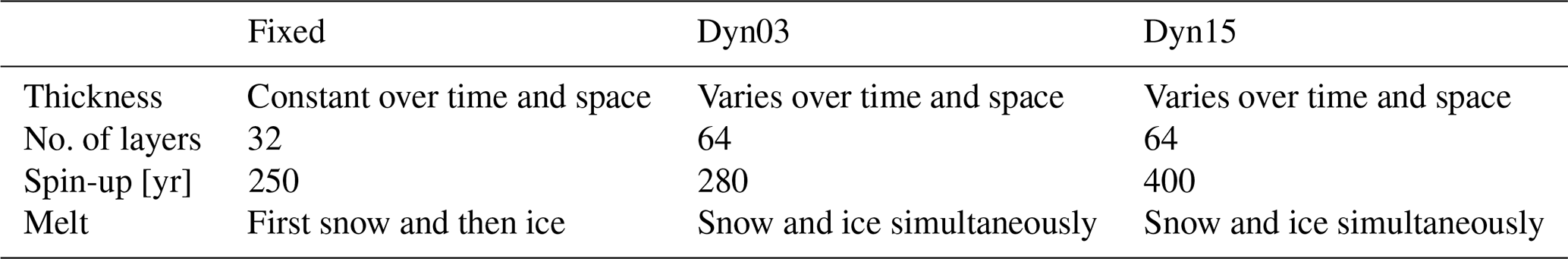
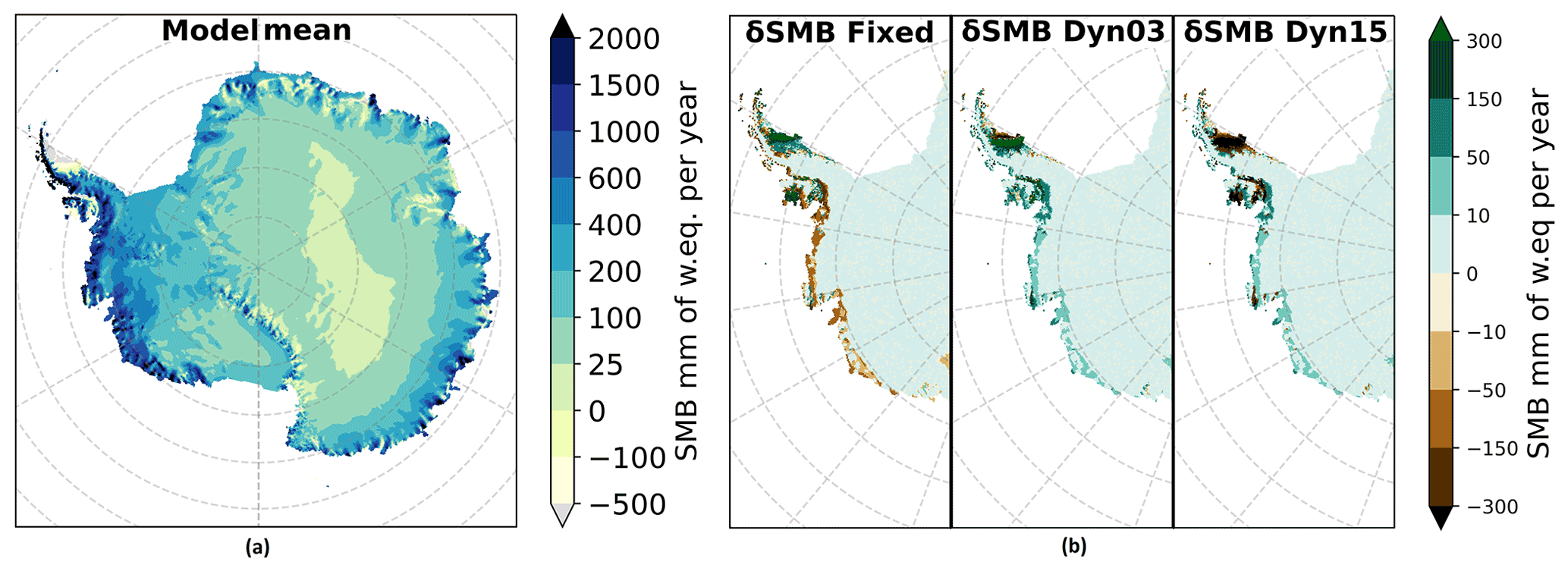
Figure 1Mean SMB from 1980 to 2017 in mm yr−1 of w.e. (a) The mean of the model mean; note the nonlinear colour bar. (b) West AIS where the δSMB has the largest differences between model versions (model minus ensemble mean).
2.4 Regional drivers and mass balance
The SAM is characterized in Fogt and Bromwich (2006) as the zonal pressure anomalies in the high southern latitudes having opposite sign to those of the midlatitudes. The SAM drives the westerly winds around Antarctica, but the stream oscillates north–south. The SAM can have three phases: positive, neutral, or negative, where positive creates a higher pressure over the midlatitudes and lower pressure over Antarctica and thus moves the westerly winds closer to Antarctica. A negative SAM creates a lower pressure over the midlatitudes and a higher pressure over Antarctica, moving the westerly winds north. When neutral there is no pressure difference anomaly. To investigate how the phase of SAM affects the SMB, monthly SAM data, as calculated by Marshall (2018), have been used. From 1980–2017, 261 months showed a positive SAM (SAM+), 193 months showed a negative SAM (SAM−), and 2 months were neutral. The SAM data are given as one monthly number, i.e. one number for the entire Antarctic domain. To see whether there is a link between SAM and SMB, the monthly SMB values were divided into two groups: SAM+ and SAM−. Then the mean SMB for all months with SAM+ was subtracted from the mean SMB for the entire period and likewise for SAM−. To examine whether there was a statistically robust difference in the δSMB signals, we performed a bootstrapping analysis, using 1200 random resamplings without replacement of the SAM data, to see whether the δSMB signals could be replicated randomly and if it could be produced randomly whether the signal would not be robust. Statistically robustness has been defined as δSMB values falling outside the 5th–95th percentile range. In order to maintain the seasonal variability in the SMB, the SAM data were shuffled in sets of 12 – in this way the order of the months was maintained and thus the seasonal cycle retained. Then confidence intervals were determined as the 5th and 95th percentiles of the distribution of the resampled δSMB values.
Observing the mass balance can be helpful to assess the spatial patterns of SMB and evaluate the modelled results. Mass balance can be derived from gravimetric measurements from space. Here GRACE/GRACE-FO mass loss time series data were computed for the period 2002–2020, using a mascon approach based on CSR R6 level-2 data, complete to harmonic degree 96 (Forsberg et al., 2017). The lowest-degree terms were substituted with satellite laser ranging data and glacial isostatic adjustment corrections from the model of Whitehouse et al. (2012). From Eq. (1) we know that MB should be equal to SMB minus discharge (SMB − D). So to evaluate our SMB model performance, GRACE and SMB − D have been plotted. The discharge values were derived from two studies: Gardner et al. (2018) and Rignot et al. (2019). Gardner et al. (2018) gave values from 2008 and 2015; here we took the mean value and used DGardner over the period. Rignot et al. (2019) have derived decadal mean discharge values from 1999–2010 and 2010–2017; for DRignot the relevant discharge values were used. The SMB value used here is for the grounded AIS only, and since the modelled SMB values are quite similar over the grounded AIS, it is only shown here for the Dyn15 simulation.
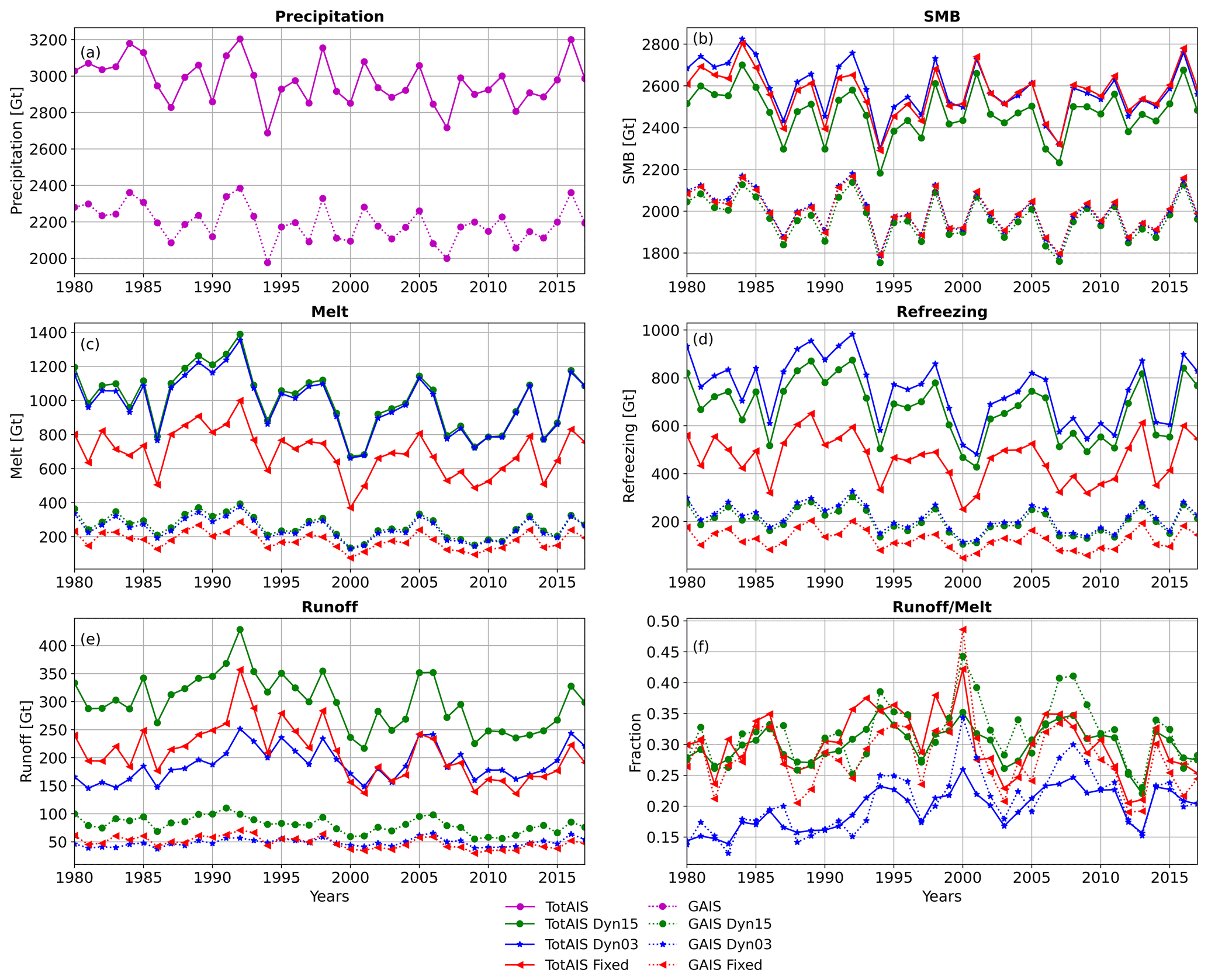
Figure 2Integrated precipitation (a), SMB (b), melt (c), refreezing (d), and runoff (e) all in Gt yr−1. Panel (f) shows the runoff to melt fraction. For the three model simulations, for the entire AIS with ice shelves (ToAIS), and for the GAIS. Note different values on the y axis.
In the model mean (1980–2017) of the three SMB simulations (Fig. 1a), we see that the majority of the total AIS (ToAIS) has a positive SMB; only a few regions show a negative SMB: Larsen ice shelf, George IV ice shelf, coastal regions of Queen Maud Land, the Transantarctic Mountains, near Amery ice shelf, and some coastal areas in East Antarctica. Near Vostok in East Antarctica, the SMB is less than 25 mm w.e. yr−1. The SMB increases towards the coast due to higher precipitation. The highest SMB is greater than 2000 mm w.e. yr−1 and is found on the windward (western) side of the AP, whereas the most negative SMB, −500 mm w.e. yr−1, is found on the leeward (eastern) side of the AP (Fig. 1a). All the model simulations show nearly identical SMB values over the GAIS; however they differ the most near the coast in West Antarctica and the AP as Fig. 1b shows. Here, we see that δSMB (model minus mean) shows that the Fixed version has a higher SMB of up to 550 mm w.e. over the Larsen ice shelf relative to the model mean. In Dyn03 the SMB values differ between −350 and 400 mm w.e. from the model mean. This change occurs over a few grid cells. In Dyn15 the SMB differs up to −650 mm w.e. compared to the model mean over the Larsen ice shelf. Since the Fixed version is above the model mean, over the Larsen ice shelf, and Dyn15 is below the model mean, it looks like the rapid change from negative to positive δSMB in Dyn03 over Larsen ice shelf is due to lack of spin-up. Below the AP, off the coast of Ellsworth Land and Marie Byrd Land, the Fixed version models a lower (−75 mm w.e.) SMB than Dyn03 (35 mm w.e.) and Dyn15 (50 mm w.e.) all relative to the model mean. Around Alexander Island in the Bellingshausen Sea, both the Fixed and Dyn15 versions have a lower SMB compared to Dyn03. The differences in spatial distribution show that in areas where melt occurs, the SMB is very sensitive to which subsurface scheme is used.
The model differences are seen in the integrated values for precipitation, SMB, melt, refreezing, and runoff, for both ToAIS and the GAIS (Fig. 2), and summarized in Table 2. As all model simulations are forced using the same precipitation field (Fig. 2a) and since the precipitation is the main driver of the SMB, the variability of the modelled SMB closely follows the precipitation variability. The spread in modelled mean melt, refreezing, and runoff are respectively 1 %, 11 %, and 8 % smaller when including the ice shelves compared to only taking the GAIS, whereas the spread in mean SMB becomes 3 % greater. To better compare the melt, refreezing, and runoff from the different simulations, the fraction of runoff to melt is shown in Fig. 2f. Dyn03 has the smallest runoff fraction whereas Dyn15 and Fixed are quite close to each other. This implies that even though the magnitudes between the simulations are quite different, the refreezing capacity of the Fixed and Dyn15 versions are near equal, and Dyn03 has the smallest refreezing capacity. Note also that the melt is 289 and 309 Gt yr−1 higher in Dyn03 and Dyn15 respectively, compared to the Fixed model. Again this is focused largely over the ice shelves, especially over the Larsen and Amery ice shelves where Dyn03 and Dyn15 have more bare ice and thus a lower albedo.
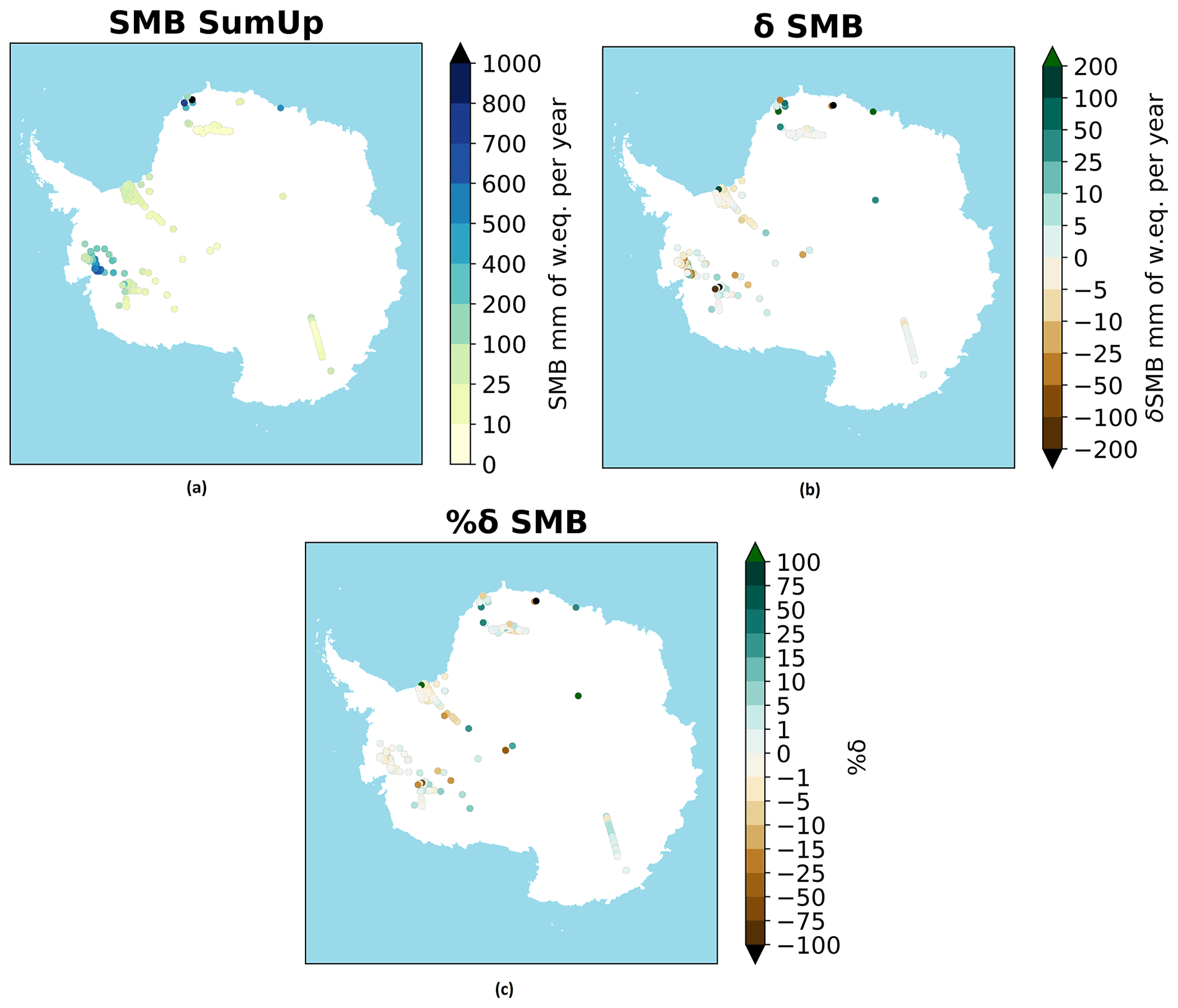
Figure 3(a) The SMB from SumUp. (b) The δSMB (SumUp minus model ensemble mean) and (c) the change in percent.
Table 2Yearly mean SMB, melt, refreezing, runoff, precipitation, and runoff fraction (runoff over melt), ± with respective standard deviations, for both the total ice sheet (ToAIS) and the grounded ice sheet (GAIS). Note that all the model simulations are forced with the same precipitation.

3.1 Evaluation against observations
Koenig and Montgomery (2019) have, in the SumUp dataset, collected accumulation rates over Antarctica. Here we evaluated the modelled SMB values against the SumUp accumulations assuming that over most of the AIS accumulation is nearly equivalent to SMB. The SumUp dataset has yearly measurements for some locations and mean values for longer periods for other locations. To make it consistent, we computed the yearly mean at each location, shown in Fig. 3a, and compared it with the nearest grid cell in the ensemble mean for the period from 1980 to 2017. If there was more than one measurement in one grid cell, an average was used (Fig. 3b). Lastly, we computed the change between the observations and the ensemble mean in percent (Fig. 3c). In total 2221 measurements have been used, located in 251 different grid cells. The SumUp accumulation dataset has areas with a high concentration of measurements, like Marie Byrd Land, Dronning Maud Land, and Dome Charlie; however, in East Antarctica there are larger areas that are not represented in the SumUp dataset. The accumulation ranges from near 0 to 100 mm w.e. yr−1 at the South Pole, Dronning Maud Land, and Dome Charlie and up towards 1000 mm w.e. yr−1 in Marie Byrd Land and the coast of Dronning Maud Land. Figure 3b shows the difference between the model ensemble mean and the in situ observations where it is seen that there are some large numerical differences in Marie Byrd Land and near the coast in Dronning Maud Land. Figure 3c displays the difference in percent for the δSMB; it shows that only three of the 251 grid cell comparisons have a difference greater than ±100 %. Furthermore half of the 251 comparison points fit within ±13 %.
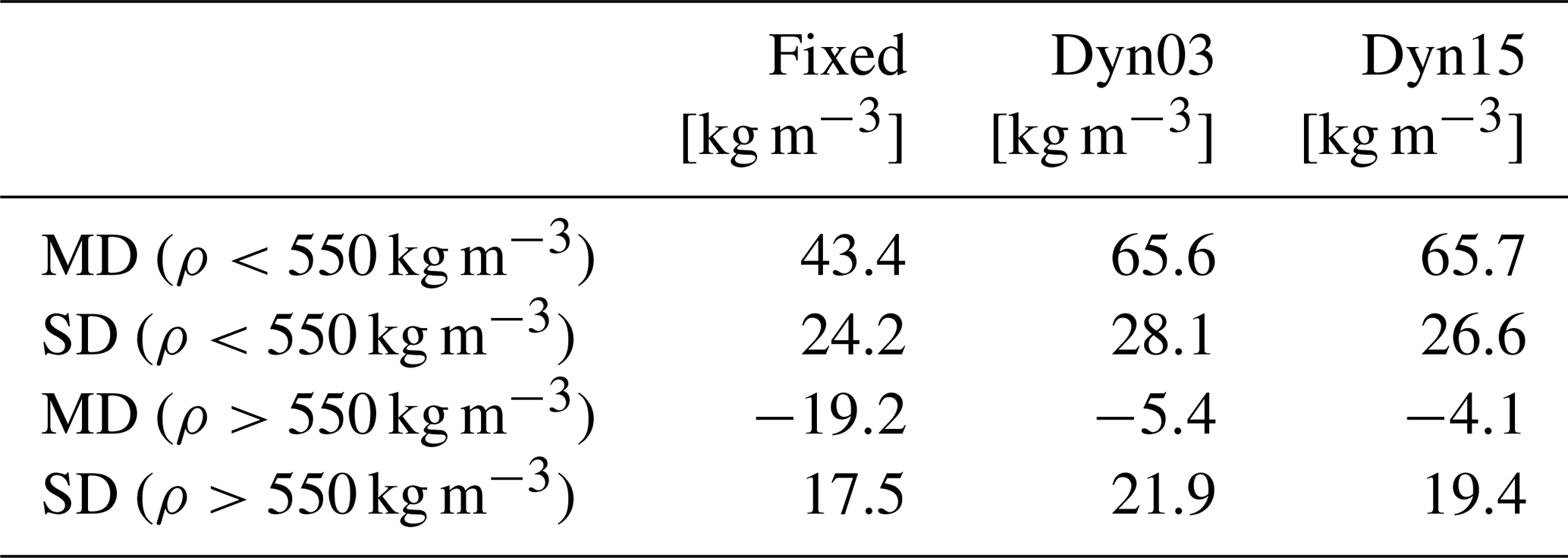
Modelled firn densities are evaluated using the SumUp dataset (Koenig and Montgomery, 2019). When disregarding firn cores shallower than 2 m, there were 139 density profiles left (Fig. 4). All the references for the firn profiles can be found in the reference list. These profiles vary in depth, from a few metres to 100 m, but the majority are drilled to 10 m depth. Knowing the coring date, we compare it to the modelled density of the nearest grid cell on the same date. Before the inter-comparison, the modelled and observed density profiles were interpolated to the same vertical resolution (if the model resolution is higher than the core resolution, the model is interpolated to fit the core resolution and vice versa). In the SumUp dataset 96 profiles had the exact date given, and seven SumUp profiles only had year and month given. Here the modelled mean density of the given month was compared. Finally 36 cores had only the year given; in these cases the modelled mean density of January was compared, as we assume they were most likely collected in the middle of the standard Antarctic summer field season. To evaluate the model performance we calculate mean difference (MD) and standard deviation (SD) between the modelled and observed firn densities. A statistical comparison of the mean difference and 1 standard deviation between the firn cores and the modelled densities is given in Table 3 for the three simulations. Summed up over the AIS, all simulations overestimate the densities below 550 kg m−3 and underestimate the densities above 550 kg m−3. It is seen that the Fixed version outperforms Dyn03 and Dyn15 for densities below 550 kg m−3. Conversely, Dyn03 and Dyn15 outperform the Fixed version for densities above 550 kg m−3. All three simulations show the best statistics for higher densities. The agreement with the in situ cores also varies spatially (Fig. 5). Generally the spatial density bias is consistent between the models.
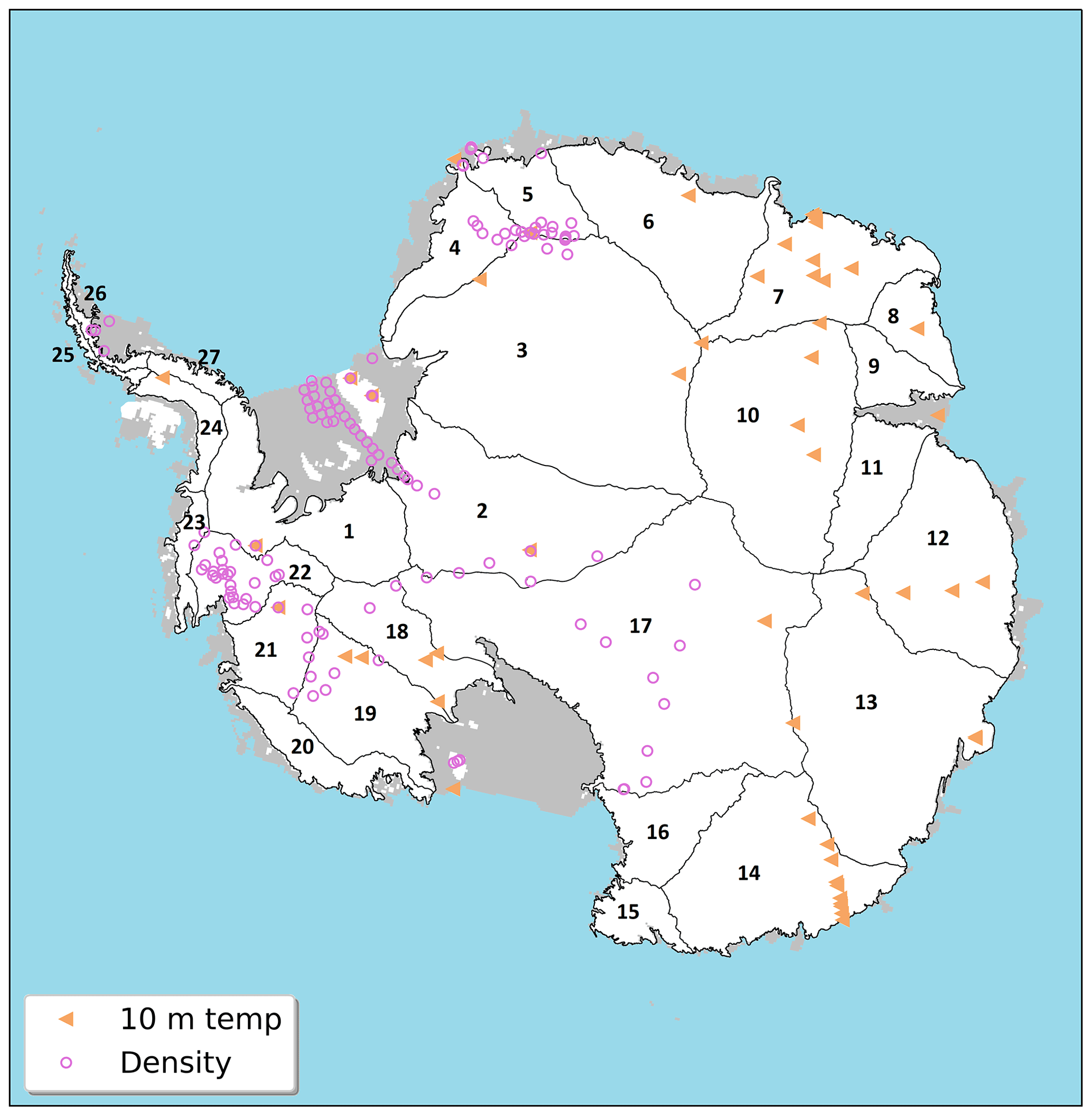
Figure 4The white colour shows the GAIS, and the grey colours show the locations of ice shelves. The spatial distribution of observations are shown with light brown triangles for borehole temperatures and magenta circles for the location of the density profiles. The grounded basins are derived from Zwally et al. (2012) and outlined by black lines.
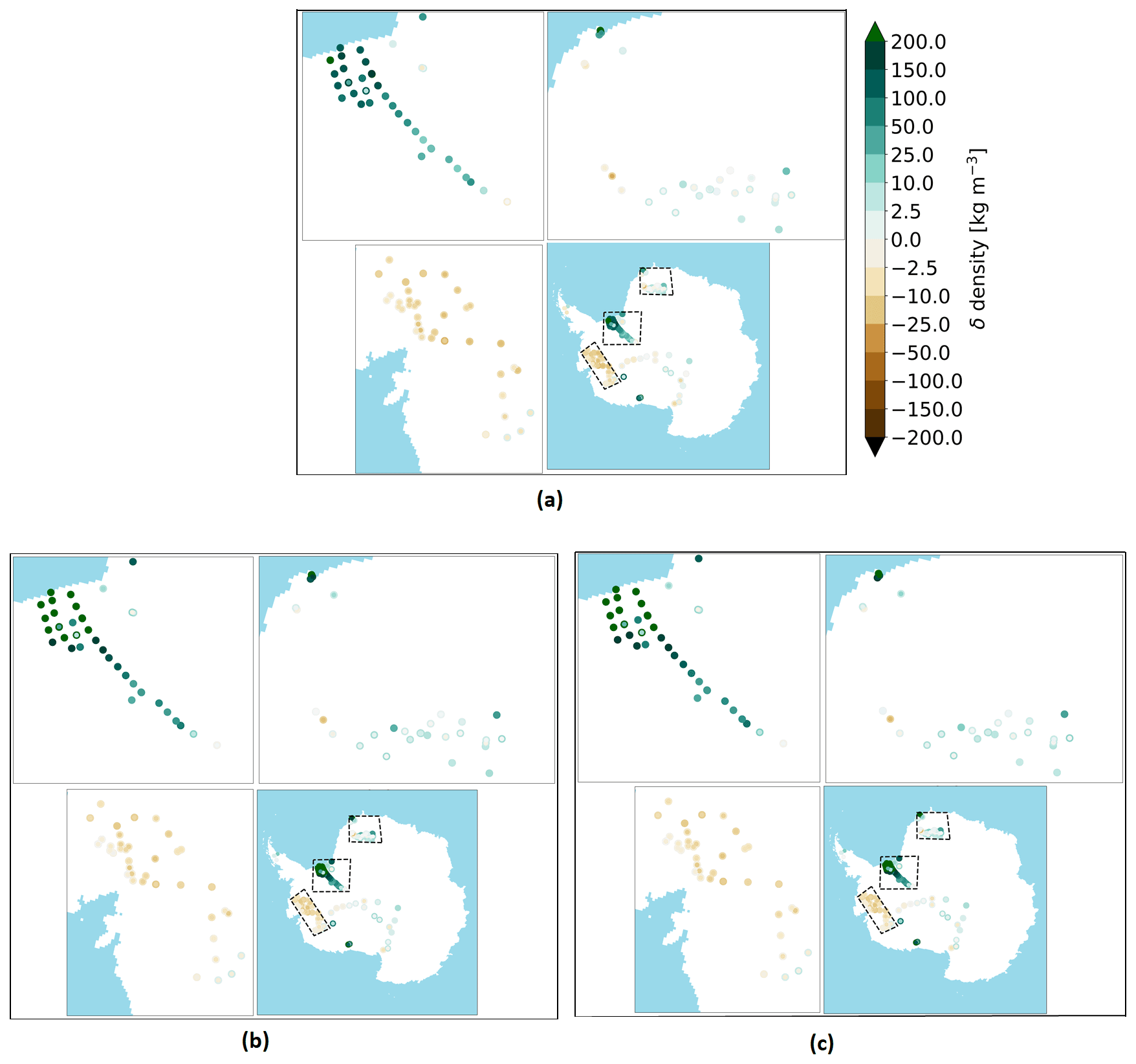
Figure 5The density bias between simulations and the observations (model minus core). The outer ring represents densities less than 550 kg m−3, and the inner circle represents densities greater than 550 kg m−3. Panel (a) is the Fixed model, (b) is Dyn03, and (c) is Dyn15. Each panel shows the entire AIS with three dashed black boxes. Each box outlines a zoom-in area: from east to west the Dronning Maud Land, Filchner–Ronne ice shelf, and Marie Byrd Land. All panels have the same colour bar.
Table 3Mean difference between the modelled and observed firn densities (model – core) and standard deviation of the modelled densities above and below 550 kg m−3. In total 139 cores were used; see Fig. 4 for locations.
Over the Filchner–Ronne ice shelf, in Dronning Maud Land and in Marie Byrd Land the distribution of profiles are quite dense; these areas are marked with boxes (Fig. 5). All simulations overestimate the density of firn over the Filchner–Ronne ice shelf. Of the 36 cores on the Filchner–Ronne ice shelf, only two have underestimated densities in the simulations. The rest of the cores have overestimated densities from 2.5 and up to 200 kg m−3. In general all three simulations have the largest biases in this region. If the cores on the Filchner–Ronne were not included in the statistics, the mean deviation for densities below 550 kg m−3 would be between 36–38 kg m−3; for densities above 550 kg m−3 the mean deviation would not change much. Mottram et al. (2021) show that the HIRHAM5 model estimates higher precipitation over the Filchner–Ronne ice shelf than other RCMs, and the overestimate in density may therefore relate to overestimated precipitation in this area, which is compliant with our Fig. 3. However, as they also note, the lack of continuous SMB observations makes it difficult to be certain if and by how much precipitation is overestimated in this region. It could also be due to an overestimation for melt and refreezing over the ice shelf.
In Dronning Maud Land there are 30 cores with a very small bias. The majority of the core densities agree within ±25 kg m−3, apart from three cores near the coast that are overestimated by 100 kg m−3 in all three simulations.
Marie Byrd Land shows a general pattern of underestimated densities in 37 cores in all simulations. However, Dyn03 and Dyn15 have lower biases compared to the Fixed. In Dyn03 and Dyn15, four cores were underestimated by more than 25 kg m−3, compared to five cores in the Fixed model. Both Dyn03 and Dyn15 have six cores where the mean deviations are between 0 and 2.5 kg m−3 for densities less than 550 kg m−3, but they underestimate densities greater than 550 kg m−3, with a mean deviation between 10 and 25 kg m−3.
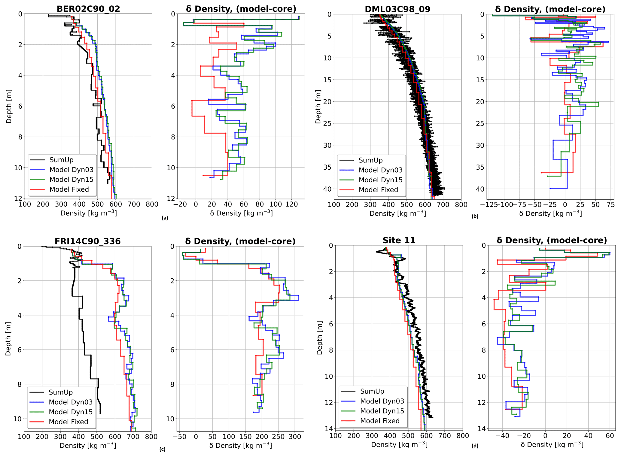
Figure 6Examples of density profiles. In each of the four subfigures, the left-hand plot shows the firn core in black and the modelled density from Fixed, Dyn03, and Dyn15 in red, blue, and green. The right-hand plot shows the difference. The cores are (a) BER02C90_02 taken in 1990 (Wagenbach et al., 1994), (b) DML03C98_09 taken in 1998 (Oerter et al., 2000), (c) FRI14C90_336 taken in 1990 (Graf and Oerter, 2006), and (d) Site 11 taken in 2013 (Morris et al., 2017).
For the Ross ice shelf cores and near the South Pole, the Fixed simulation overestimates most of the cores, some of them by 50 to 100 kg m−3 for densities less than 550 kg m−3 and more than 100 kg m−3 for densities greater than 550 kg m−3. However, for Dyn03 and Dyn15 we also observe an overestimation of most cores, but only six of them are overestimated by more than 25 kg m−3.
Figure 6 shows 4 of the 139 firn cores: core BER02C90_02 (Wagenbach et al., 1994) (Fig. 6a), core DML03C98_09 (Oerter et al., 2000) (Fig. 6b), core FRI14C90_336 (Graf and Oerter, 2006) (Fig. 6c), and core Site 11 (Morris et al., 2017) (Fig. 6d). These four cores are selected because they are located in different regions of the AIS, and, furthermore, they show different examples of under-/overestimations of modelled densities. The Fixed simulation fit quite well (±20 kg m−3) with the core taken on Berkner Island (Fig. 6a), whereas Dyn03 and Dyn15 show a larger bias mainly at the surface and the top 3 m of the firnpack. The core from Dronning Maud Land (Fig. 6b) has a high vertical resolution; the deeper the cores go, the smaller the biases become. Cores FRI14C90_336 and Site 11 are taken on the Ronne ice shelf and in Marie Byrd Land respectively. The model densities in FRI14C90_336 are overestimated below 1 m depth, and the mean bias is 200 kg m−3. At Site 11 all simulations underestimate the density; however below 2 m depth, the underestimation is nearly constant with a mean bias of −20 kg m−3.
The modelled subsurface temperatures are evaluated against observed 10 m firn temperature measurements from 49 boreholes (van den Broeke, 2008) (see Fig. 4 for the locations). Most of the temperatures were taken in the 1980s and 1990s; however only the year or decade is known for when these were taken. Therefore they are compared with the modelled mean 10 m firn temperature from 1980–2000. We evaluated the model performance using the root-mean-square difference (RMSD), mean difference (MD), and coefficient of determination (R2). Subsurface temperatures are only sparsely available in Antarctica. The measured 10 m firn temperatures are compared with the modelled mean 10 m firn temperature of the nearest grid cell (Fig. 7). The red, blue, and green lines are the regression lines of first order, for Fixed, Dyn03, and Dyn15; they have an R2 of 0.98, 0.97, and 0.98, respectively. It is assumed that the in situ temperatures are true, so the errors are in the modelled temperatures. For temperatures below −30 ∘C the three simulations are in agreement, but in warmer firn temperatures > −30 ∘C, the agreement becomes worse. The mean deviation of the three model simulations is listed Table 4.
Table 4Mean deviation, root-mean-square deviation, and coefficient of determination, for the modelled and observed 10 m temperature.
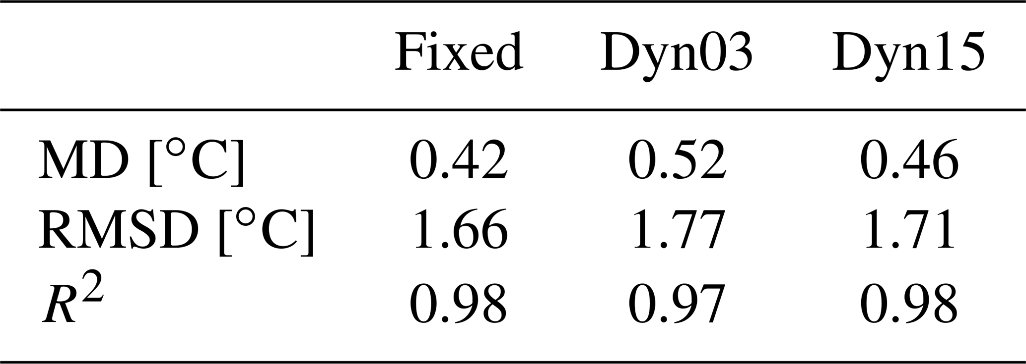
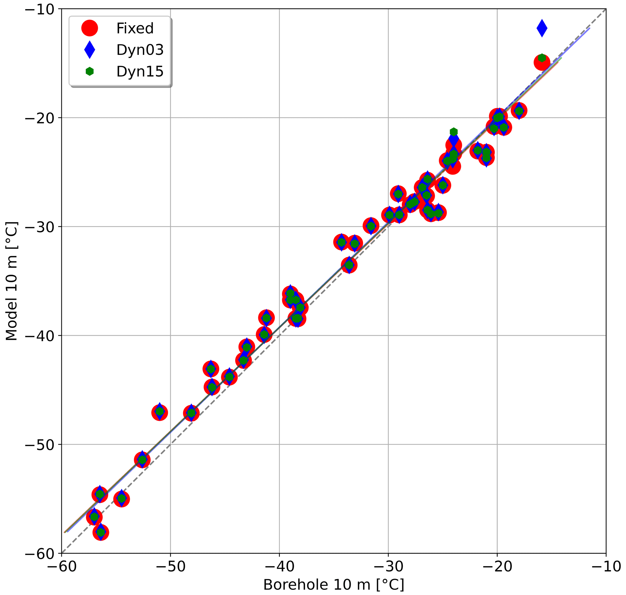
Figure 7The dots are 10 m temperature from boreholes vs. mean model 10 m temperature. The solid lines are the regression lines of first order, and the grey dashed line shows the diagonal.
The annual SMB for the three simulations (Table 2) is of the same magnitude as the previous HIRHAM5 SMB estimate of 2659 Gt yr−1 for the ToAIS (Mottram et al., 2021). However, we model a lower SMB, with only Fixed and Dyn03 within 1 standard deviation range of Mottram et al. (2021). The lower SMB estimates are due to the inclusion of the runoff component in the SMB calculation. The initial SMB results from HIRHAM5 in Mottram et al. (2021) were only calculated from precipitation, evaporation, and sublimation. Calculating the SMB by including a subsurface model results in a more realistic SMB, due to the fact that it takes surface and subsurface processes like energy fluxes, meltwater percolation, and refreezing into account.
The spatial distribution of SMB fits reasonably well compared with the SumUp accumulation measurements; however, more measurements, especially in East Antarctica, are needed to be able to do a complete evaluation. Furthermore, the spatial distribution of SMB broadly agrees with other studies (Van de Berg et al., 2005; Krinner et al., 2007; Agosta et al., 2019; Souverijns et al., 2019). However, the total integrated mean SMB in these published studies differs, likely due to a number of different reasons. The ice mask, model resolution and domain, and nudging (if any) are identified as a source of differences in Mottram et al. (2021). However, differences in model parameterizations affecting components such as sublimation and precipitation are also important. For example, the modelled annual mean precipitation in HIRHAM5 is 2971±122 Gt, in COSMO-CLM2 it is 2469±78 (Souverijns et al., 2019), and in RACMO2.3p2 it is 2396±110 Gt (van Wessem et al., 2018). However, the geographical distribution of precipitation is uneven between these models, with COSMO-CLM2 being much drier in western Antarctica than other models in the comparison. Even using a common ice mask, Mottram et al. (2021) found that the difference in precipitation is around 500 Gt yr−1 between HIRHAM5 (the wettest model) and COSMO-CLM2 (the driest model in the intercomparison). The high precipitation in regions of high relief in HIRHAM5 is attributed to a wet bias in the precipitation scheme, also identified in southern Greenland and similarly occurring in the RACMO2.3p2 regional climate model (Hermann et al., 2018). In both models this wet bias in steep topography is related to the precipitation and cloud micro-physics schemes (Mottram et al., 2021). Areas with a negative SMB can be due to large melt rates, which is what we see in the model over the Larsen ice shelf with melt values between 1200 and increasing toward the west to 2300 mm w.e. yr−1 and SMB values in the range of 300 to 1800 mm w.e. yr−1 increasing toward the west. In general all three simulations display a higher melt compared to other RCM studies, e.g. 71 Gt yr−1 in RACMO2.3p2 (van Wessem et al., 2018) or 40 Gt yr−1 in MARv3.6.4 (Agosta et al., 2019). These two numbers are without the AP, but they are nevertheless very low compared to our melt rates. Trusel et al. (2013) derived satellite-based melt rate estimates from 1999 to 2009, and over that period, the Larsen ice shelf experienced the largest melt of around 400 mm w.e. yr−1. However, these estimates were derived using RACMO2.1, and the satellite detects melt areas on the Larsen ice shelf that were not simulated in RACMO2.1, most likely due to coarse resolution, so 400 mm w.e. yr−1 might be on the low end. Nevertheless, Trusel et al. (2013) estimates are still 3 to 6 times lower than our simulation. This suggests that the subsurface model may compute a melt rate that is too high in at least some locations.
Negative SMB values can also be due to high sublimation rates in, e.g., blue ice areas (Hui et al., 2014). For example, Kingslake et al. (2017) found blue ice in Dronning Maud Land and near the Transantarctic Mountains. In these areas our SMB model mean also shows negative SMB between −50 and −400 mm w.e. yr−1. A closer investigation (not shown) reveals that the negative SMB values in these areas are driven by the sublimation and thereby consistent with the creation of blue ice areas.
The differences in SMB between the model simulations (Fig. 1b) are largest near the coast in West AIS and especially on the Larsen ice shelf. This is confirmed in Fig. 2b, where the difference in integrated SMB between the model simulations is greater when the ice shelves are included. We attribute the differences between the Fixed and Dyn models to the following differences in model designs. The increased vertical resolution in the Dyn models, with a higher vertical resolution (the top layers can be 6.5 cm w.e. thick) means that the cold content in the upper layers is depleted faster, and it starts to melt while the layer below is potentially still below freezing. Conversely the top layers in the Fixed model get thicker rather quickly, which means it takes longer to be brought to melting point and start melting. Furthermore, the two versions of the subsurface model have different melting schemes. In both versions one layer can contain snow and ice at the same time, described with a fraction. However, in the Fixed model snow melts first and then, if there is more energy left, the ice melts. Conversely, the Dyn melts snow and ice simultaneously. This simultaneous melting of snow and ice was introduced in the Dyn version to prevent the top layer from being depleted of its snow content and left only with ice (Vandecrux et al., 2018). A top layer composed of ice would then prevent surface melt from infiltrating below the top layer. By melting snow and ice simultaneously, there is always snow in the top layer for meltwater infiltration to happen. This difference of infiltration may cause the snowmelt to refreeze less and more water to run off than the simultaneous melt of snow and ice. To investigate these differences in melt, refreezing, and runoff, the runoff fractions have been plotted in Fig. 2f and listed in Table 2. Here it is seen that even though the difference in melt between Dyn03 and Dyn15 is only around 20 Gt yr−1, the difference between the runoff and melt fractions is larger. The Fixed model melts around 300 Gt yr−1 less than the dynamical versions, but the runoff-to-melt ratio is the same for Fixed and Dyn15. This means that Fixed and Dyn15 have the same relative runoff, leading to the same relative refreezing, indicating that this difference does not cause a significant partition of melt between refreezing and runoff.
The difference in SMB between the three simulations confirms how complex it is to estimate the SMB. Just by changing the subsurface scheme, the final result differs by 90 Gt yr−1. By keeping the same subsurface scheme and changing the spin-up length, the final result differs by 110 Gt yr−1. These changes in SMB illustrate the consequences of including dynamic firn processes since the layer density and temperature and other firn properties are better conserved, potentially allowing more retention and refreezing where there is capacity or reducing it where there is not. Although these differences are currently only a few percent of the total SMB, as the climate warms and melt becomes more widespread in Antarctica (e.g. Boberg et al., 2020; Kittel et al., 2021), accounting for these processes will become more important. Moreover, on local and regional scales, the differences are more important when determining mass balance in basins or outlet glacier/ice shelves.
The differences between versions with a different spin-up period suggest that the snowpack is not quite in equilibrium in all locations. Therefore, SMB calculations consequently vary due to the amount of melt calculated during the initialization period. Retention and refreezing of meltwater during spin-up cause different profiles of temperature and density to develop depending on how long the spin-up lasts. These results therefore emphasize the importance of adequate spin-up and assessment of the effects of snowpack spin-up in producing and using SMB in Antarctica.
Vandecrux et al. (2020b) found that the Fixed version smoothes the firn density profiles, when compared to the dynamical version; this is confirmed by our results. One of the criteria for the dynamical version is that it prefers to merge layers deeper than 5 m of water equivalent, meaning that the top 5 m w.e. has a high vertical resolution, which makes it easier to detect changes in density. In areas such as the AP, Ronne–Filchner ice shelf, Ross ice shelf, and coastal areas of Dronning Maud Land where seasonal melt occurs (Zwally and Fiegles, 1994; Wille et al., 2019), meltwater can percolate into the firn and refreeze, creating ice lenses that change the density but that cannot be detected if the subsurface scheme has layers with a fixed mass even if the vertical resolution is increased (Vandecrux et al., 2020b). Not only is there a difference between the models when evaluating density profiles, but this study also shows the importance of spatial evaluation. Here the three simulations follow the same pattern by over-/underestimating the densities in the same areas (Fig. 5). This systematic bias may indicate either further tuning of densification routines is necessary or that there are systematic biases in accumulation, leading to these errors. The subsurface scheme does not currently incorporate wind-blowing snow processes that may prove important in correcting biases in accumulation. On the other hand, although 0.11∘ is a high-resolution model in Antarctica and thus better captures topographic variability than lower-resolution models, it is still relatively coarse when it comes to capturing steep topography. Errors in orographic precipitation are difficult to measure even in well-instrumented basins and are poorly captured in Antarctica where observations are few and far between. The densification bias becomes especially important when using altimetry data to estimate the total MB, like in Shepherd et al. (2018) and Rignot et al. (2019). Here the firn densification rate is needed to correct the altimetry data (Griggs and Bamber, 2011).
Since the density cores are primarily taken from West Antarctica and Dronning Maud Land, these statistics represent complex areas with high precipitation and melt–refreezing events, whereas density comparisons from less complex areas (low precipitation and no melt–refreezing) such as East Antarctica are sparse. Nonetheless they are still very important. Based on the statistics from these model set-ups, the Dyn version is preferred when modelling densities above 550 kg m−3.

Figure 8Integrated relative mass change over the grounded Antarctic Peninsula (a), the grounded West AIS (b), grounded East AIS (c), and the GAIS (d). GRACE relative mass change from 2002 to 2020 (black graph). SMB minus discharge (green/red graphs). SMB values are from the Dyn15 simulation, and discharge values are derived by Gardner et al. (2018) (in green) and Rignot et al. (2019) (in red). Note that the y axis differs from panel to panel.
The simulated 10 m firn temperature depends on the thickness and number of layers above the 10 m point. The thickness of a layer determines how conductive heat fluxes are resolved in the near-surface snow. A thicker layer will have more thermal inertia and will require more energy to be warmed up. A thin layer can respond much more quickly to fluctuations in the surface energy balance. Differences in simulated temperatures between models, as we see in Table 4, can therefore be explained by vertical resolution, which affects both their calculation of temperature and how the heat is conducted to a depth of 10 m. Note that the models also use different thermal conductivity parameterizations.
4.1 Satellite gravimetric mass balance
Over the AP there is a large disagreement between SMB − DGardner and SMB − DRignot, the mean discharge values differ by 90 Gt yr−1, with DRignot being the largest. This results in opposite trends of SMB − D. SMB − DGardner shows a mass gain of around 600 Gt, and SMB − DRignot shows approximate mass loss of 1150 Gt over the period, whereas GRACE has a mass loss of around 400 Gt for the period (Fig. 8a). There are times when the variability between GRACE and the two SMB-D graphs follows each other, e.g. local peak around year 2006, 2011, and 2017. Since the discharge is plotted as a constant, this variability originates from the SMB model, most likely precipitation. This means that the DGardner value is too small, DRignot values are too large, or the SMB magnitude is too low or high depending on which discharge is used. As the resolution of GRACE is quite coarse, it can add to the uncertainties over the AP, because of narrow topography. Over the grounded West AIS the trend of GRACE, SMB − DRignot, and SMB − DGardner agrees. They all see a mass loss, of around 2000, 2150, and 1700 Gt, respectively, for the overlapping period (Fig. 8b). The discharge values from the two studies differ only by 2 Gt yr−1 from 2002 to 2010 but by 50 Gt yr−1 from 2010 to 2017, with DGardner being the lowest. GRACE measures a smaller mass loss in the beginning of the period, and then around 2009 the GRACE mass loss increases. Both Gardner et al. (2018) and Rignot et al. (2019) have found an increasing discharge in West Antarctica. However due to the limited temporal resolution from Gardner et al. (2018), the discharge is assumed constant, resulting in an equal offset in SMB − D from 2002–2009, but then diverging results from 2010. This shows that in areas where there are large changes in the dynamic mass loss, discharge values with a higher temporal resolution are needed.

Figure 9SMBa (monthly values minus mean values) in months for SAM− (a) and SAM+ (b), for each basin. The vertical dashed lines split the basins into areas. Starting from the left, we show basins towards the Weddell Sea, Dronning Maud Land, eastern coast, Ross Sea, western coast/Amundsen Sea, and Bellingshausen Sea. The thin bars are the 5th and 95th percentiles, for the bootstrapping analysis with 1200 runs. Locations of the basins can be seen in Fig. 4. In basins where the SMBa values fall outside the percentiles, there is a robust relationship between the SMB and SAM.
Over the East GAIS the agreement between GRACE and SMB − DGardner is remarkably good. Between 2009 and 2011 large snowfall events were observed in Dronning Maud Land (Boening et al., 2012; Lenaerts et al., 2013) (basins 5–8 in Fig. 4). These snowfall events led to rapid mass gain, which is seen in both GRACE and SMB − DGardner, especially in 2009–2010 (Fig. 8c). This mass gain is less pronounced in SMB − DRignot because it estimates an overall mass loss for the period. In the SMB signal there are yearly variabilities; however, these variabilities are larger in the GRACE data compared to SMB − D. For the entire GAIS GRACE detects a mass loss of 900 Gt, SMB − DGardner shows a mass gain of 500 Gt, and SMB − DGardner shows a mass loss of 4000 Gt, for the overlapping period 2002–2017. The majority of that difference between GRACE and SMB − DGardner can be attributed to the AP. The difference between GRACE and SMB − DRignot arises from the AP and East GAIS.
4.2 Circulation effects on SMB and the Southern Annular Mode
We observe a robust (outside the 5th–95th percentile range) relationship between SMB and SAM in 13 out of the 27 basins (Fig. 9a and b). For each phase of the SAM, SMB anomalies (SMBa) are defined as the SMB in months with a SAM− or SAM+ monthly mean minus SMB over the full period. The SMBa for SAM−, when the westerlies are further away from the Antarctic continent, shows magnitudes well outside the percentiles for all model simulations. Basins 2 and 3 that have outlets to the Filchner–Ronne ice shelf (EAIS); basin 4 in Dronning Maud Land (EAIS); basin 7 in Enderby Land (EAIS); basins 9, 10, and 12 surrounding the Amery ice shelf (EAIS); basins 17, 18, and 19 with an outlet into Ross ice shelf; basin 20 in Marie Byrd Land (WAIS); and basins 24 and 25 located on the windward side of the AP are particularly affected by SAM−. For SAM+, when the westerlies are closer to the continent the SMBa magnitudes are generally smaller and have an opposite sign; however we see the same pattern in the same basins as for SAM−. A SAM+ phase results in a relatively low pressure over the AIS compared to the midlatitudes, and we see a negative SMBa in 16 of 27 basins, namely 6, 9–13, 15–23, and 26 (Fig. 9b). Marshall et al. (2017) reported a similar signal for precipitation, which confirms our results since precipitation is the main driver of SMB. Basin 26 shows a negative SMBa, and basin 27 has a slightly positive SMBa, which is due to the steep orography on the windward side of the AP creating a shadowing effect on the leeward side of the AP. For SAM− the SMBa signal is opposite, and the mean magnitude of the signal is 26 % larger in all basins (Fig. 9a). During months of SAM+ the average SAM index is 1.45. Figure 9 shows that basins 1–5, 7, 14, 24–25, and 27 have SMB anomalies (SMBa) of the same sign as the SAM: SMB is 0.28 Gt per month higher than average in the case of SAM+ and 0.39 Gt per month lower than average in the case of SAM−. Those basins are mostly located in the east, Ross, and Amundsen Sea sectors. Contrastingly, basins 6, 8–13, 15–23, and 26 have SMB 0.32 Gt per month below average in months of SAM+ and 0.43 Gt per month above average in months of SAM−. These basins are mostly located in the Weddell Sea, Dronning Maud Land, and Bellingshausen sectors. For months with SAM− the average SAM index is −1.36. We can see that for SAM of similar absolute magnitude, SAM− has a stronger impact on SMB over the GAIS.
In both positive and negative SAM events basins 24 and 25 on the windward side of the AP show strong correlation between the SAM index and SMB magnitude also reported by Marshall et al. (2017). So even though the AP is narrow (50 to 300 km across) the SAM plays an important role. Comparing with Vannitsem et al. (2019), we see agreement in large parts of West Antarctica. However, it is difficult to compare in East Antarctica because we use basins, and most of them go far inland, whereas Vannitsem et al. (2019) defined narrow coastal regions and one large plateau region.
From 1980 to 2017 the SAM has become more positive (Fogt and Marshall, 2020), this positive trend in the SAM is attributed to stratospheric ozone depletion (Thompson et al., 2011; Fogt et al., 2017). If this trend continues the basins on the leeward side of the AP will see a smaller mass gain in the future, which could accelerate the collapse of the Larsen ice shelf. This is also seen in basins 9, 10, 11, and 12 surrounding the Amery ice shelf and basin 21 where Thwaites glacier is located. Not all of the above-mentioned basins show δSMB signals that are statistically robust (i.e. the signals are within the 5th or 95th percentiles), but if the trend in the positive SAM continues, it might become an important factor in the future (Fogt and Marshall, 2020).
It is thus important to take the SAM phases into account when investigating the SMB at a regional scale. Furthermore it is extremely important that global circulation models resolve the SAM realistically if future climate projections are to be used with confidence to make projections of sea level rise from Antarctica.
We estimate the Antarctic SMB to range from 2583.4±121.6 to 2473.5±114.4 Gt yr−1 over the total area of the ice sheet including shelves and between 1995.4±99.3 and 1963.3±96.2 over the grounded part, for the period from 1980 to 2017. The difference is due to different subsurface models forced with HIRHAM5 outputs. The Dyn03 version has the highest integrated SMB over the ToAIS (GAIS) at 2583.4±121.6 (1995.4±99.3) Gt yr−1, and Dyn15 has the lowest 2473.5±114.4 (1963.3±96.2) Gt yr−1. The Fixed version is ≈19 Gt yr−1 lower than Dyn03 over the ToAIS and 0.2 Gt yr−1 lower than Dyn03 over the GAIS. The simulations compute nearly equal SMB over the interior. The main differences are seen in the coastal areas of West AIS and the AP. The Dyn15 simulation gives the smallest SMB estimate and is thus closest to other studies (van Wessem et al., 2018; Souverijns et al., 2019; Agosta et al., 2019); however it is still 200–300 Gt yr−1 higher. Evaluating the modelled density profiles shows the Lagrangian model set-up has the lowest bias and standard deviation in density differences for densities greater than 550 kg m−3; for densities less than 550 kg m−3 the Eulerian performance is best. In general all models overestimate the densities on the Filchner–Ronne ice shelf and underestimate the densities in Marie Byrd Land and around the Ross ice shelf. It is therefore clear that there are regional systematic biases. To evaluate our simulated SMB, we compare our simulations with the SumUp accumulation rates. Half of the comparing sites fit with ±13 %; moreover we also compare our simulations to MB estimations (SMB minus discharge) from GRACE. We use discharge from two sources: Gardner et al. (2018) and Rignot et al. (2019). There are large differences between the discharge values over the AP, leading to our simulations overestimating MB when using DGardner and underestimating MB when using DRignot. Over the East GAIS the MB is underestimated using DRignot but fits quite well to the GRACE MB when using DGardner. These disagreements between the two observational datasets makes it hard to distinguish how well the modelled SMB fits with total mass balance estimates.
Regional precipitation is strongly linked to the phase of the SAM as shown by the bootstrap analysis. By using outputs from HIRHAM5 forced with ERA-Interim to resolve the SAM correctly, robust signals are identified in 13 out of 27 basins. It is clear that the phase of the SAM affects the spatial distribution of SMB. When SAM is negative, there is a lower SMB on the windward side of the Antarctica Peninsula and a higher SMB over the plateau and vice versa when SAM is positive. This makes the SAM an important factor to evaluate in global models when downscaling models for projecting future Antarctic climate.
A MATLAB version of the subsurface model code used in these study is available here: https://doi.org/10.5281/zenodo.4542767 (Vandecrux, 2021).
A selection of the HIRHAM5 data are available here: http://ensemblesrt3.dmi.dk/data/prudence/temp/RUM/HIRHAM/ANTARCTICA/ (Mottram and Boberg, 2021), and a selection of the subsurface model data are available here: https://doi.org/10.5281/zenodo.5005265 (Hansen et al., 2021).
More data are available by contacting nichsen@space.dtu.dk.
NH, SBS, and RM conceived the study. NH ran the subsurface model simulations with help from PLL, made the plots, and performed the analysis under guidance from RM, SBS, PLL, PT, BV, and RF. HIRHAM5 model simulation was carried out by FB and RM. The Fixed model was developed by PLL, and the dynamical versions were developed by BV and PLL. RF prepared the GRACE data. All authors contributed to writing the paper.
The authors declare that they have no conflict of interest.
Publisher's note: Copernicus Publications remains neutral with regard to jurisdictional claims in published maps and institutional affiliations.
This publication was supported by PROTECT. Data analysis was supported by the Danish state through the National Centre for Climate Research (NCKF). We also gratefully acknowledge the ESA CCI Ice Sheets project as a forum for the interchange of ideas that led directly to this study.
This project has received funding from the European Union’s Horizon 2020 research and innovation programme under grant agreement no. 869304, PROTECT contribution number 18. HIRHAM5 regional climate model simulations were carried out by Ruth Mottram and Fredrik Boberg as part of the ice2ice project, a European Research Council project under the European Community’s Seventh Framework Programme (FP7/2007-2013)/ERC grant agreement 610055. GRACE data analysis was supported by ESA Climate Change Initiative for the Greenland ice sheet funded via ESA ESRIN contract number 4000104815/11/I-NB and the Sea Level Budget Closure CCI project funded via ESA-ESRIN contract number 4000119910/17/I-NB.
This paper was edited by Alexander Robinson and reviewed by Christoph Kittel and one anonymous referee.
Agosta, C., Amory, C., Kittel, C., Orsi, A., Favier, V., Gallée, H., van den Broeke, M. R., Lenaerts, J. T. M., van Wessem, J. M., van de Berg, W. J., and Fettweis, X.: Estimation of the Antarctic surface mass balance using the regional climate model MAR (1979–2015) and identification of dominant processes, The Cryosphere, 13, 281–296, https://doi.org/10.5194/tc-13-281-2019, 2019. a, b, c, d, e
Bell, R. E., Banwell, A. F., Trusel, L. D., and Kingslake, J.: Antarctic surface hydrology and impacts on ice-sheet mass balance, Nat. Clim. Change, 8, 1044–1052, 2018. a
Boberg, F., Mottram, R., Hansen, N., Yang, S., and Langen, P. L.: Higher mass loss over Greenland and Antarctic ice sheets projected in CMIP6 than CMIP5 by high resolution regional downscaling EC-Earth, The Cryosphere Discuss. [preprint], https://doi.org/10.5194/tc-2020-331, 2020. a
Boening, C., Lebsock, M., Landerer, F., and Stephens, G.: Snowfall-driven mass change on the East Antarctic ice sheet, Geophys. Res. Lett., 39, L21501, https://doi.org/10.1029/2012GL053316, 2012. a
Calonne, N., Geindreau, C., Flin, F., Morin, S., Lesaffre, B., Rolland du Roscoat, S., and Charrier, P.: 3-D image-based numerical computations of snow permeability: links to specific surface area, density, and microstructural anisotropy, The Cryosphere, 6, 939–951, https://doi.org/10.5194/tc-6-939-2012, 2012. a
Christensen, O., Gutowski, W., Nikulin, G., and Legutke, S.: CORDEX Archive design, Danish Climate Centre, Danish Meteorological Institute, Danish Meteorological Institute. Technical Report, available at: https://is-enes-data.github.io/cordex_archive_specifications.pdf (last access: May 2020), 2014. a
Christensen, O. B., Drews, M., Christensen, J. H., Dethloff, K., Ketelsen, K., Hebestadt, I., and Rinke, A.: The HIRHAM regional climate model, Version 5 (beta), Danish Climate Centre, Danish Meteorological Institute, Danish Meteorological Institute, Technical Report, 2007. a, b
Colbeck, S.: A theory for water flow through a layered snowpack, Water Resour. Res., 11, 261–266, https://doi.org/10.1029/WR011i002p00261, 1975. a
Coléou, C. and Lesaffre, B.: Irreducible water saturation in snow: experimental results in a cold laboratory, Ann. Glaciol., 26, 64–68, 1998. a
Dalaiden, Q., Goosse, H., Lenaerts, J. T., Cavitte, M. G., and Henderson, N.: Future Antarctic snow accumulation trend is dominated by atmospheric synoptic-scale events, Commun. Earth Environ., 1, 1–9, 2020. a
Dee, D. P., Uppala, S. M., Simmons, A. J., Berrisford, P., Poli, P., Kobayashi, S., Andrae, U., Balmaseda, M. A., Balsamo, G., Bauer, P., Bechtold, P., Beljaars, A. C. M., van de Berg, L., Bidlot, J., Bormann, N., Delsol, C., Dragani, R., Fuentes, M., Geer, A. J., Haimberger, L., Healy, S. B., Hersbach, H., Hólm, E. V., Isaksen, L., Kållberg, P., Köhler, M., Matricardi, M., McNally, A. P., Monge-Sanz, B. M., Morcrette, J.-J., Park, B.-K., Peubey, C., de Rosnay, P., Tavolato, C., Thépaut, J.-N., and Vitart, F.: The ERA-Interim reanalysis: Configuration and performance of the data assimilation system, Q. J. Roy. Meteorol. Soc., 137, 553–597, 2011. a
Eerola, K.: About the performance of HIRLAM version 7.0, Hirlam Newslett., 51, 93–102, 2006. a
Feser, F., Rockel, B., von Storch, H., Winterfeldt, J., and Zahn, M.: Regional climate models add value to global model data: a review and selected examples, B. Am. Meteorol. Soc., 92, 1181–1192, 2011. a
Fettweis, X., Hofer, S., Krebs-Kanzow, U., Amory, C., Aoki, T., Berends, C. J., Born, A., Box, J. E., Delhasse, A., Fujita, K., Gierz, P., Goelzer, H., Hanna, E., Hashimoto, A., Huybrechts, P., Kapsch, M.-L., King, M. D., Kittel, C., Lang, C., Langen, P. L., Lenaerts, J. T. M., Liston, G. E., Lohmann, G., Mernild, S. H., Mikolajewicz, U., Modali, K., Mottram, R. H., Niwano, M., Noël, B., Ryan, J. C., Smith, A., Streffing, J., Tedesco, M., van de Berg, W. J., van den Broeke, M., van de Wal, R. S. W., van Kampenhout, L., Wilton, D., Wouters, B., Ziemen, F., and Zolles, T.: GrSMBMIP: intercomparison of the modelled 1980–2012 surface mass balance over the Greenland Ice Sheet, The Cryosphere, 14, 3935–3958, https://doi.org/10.5194/tc-14-3935-2020, 2020. a
Fogt, R. L. and Bromwich, D. H.: Decadal variability of the ENSO teleconnection to the high-latitude South Pacific governed by coupling with the southern annular mode, J. Climate, 19, 979–997, 2006. a, b
Fogt, R. L. and Marshall, G. J.: The Southern Annular Mode: variability, trends, and climate impacts across the Southern Hemisphere, Wiley Interdisciplin. Rev.: Clim. Change, 11, e652, https://doi.org/10.1002/wcc.652, 2020. a, b, c
Fogt, R. L., Goergens, C. A., Jones, J. M., Schneider, D. P., Nicolas, J. P., Bromwich, D. H., and Dusselier, H. E.: A twentieth century perspective on summer Antarctic pressure change and variability and contributions from tropical SSTs and ozone depletion, Geophys. Res. Lett., 44, 9918–9927, 2017. a
Forsberg, R., Sørensen, L., and Simonsen, S.: Greenland and Antarctica ice sheet mass changes and effects on global sea level, in: Integrative Study of the Mean Sea Level and Its Components, Space Sciences Series of ISSI, Springer, 58, 91–106, 2017. a, b
Fretwell, P., Pritchard, H. D., Vaughan, D. G., Bamber, J. L., Barrand, N. E., Bell, R., Bianchi, C., Bingham, R. G., Blankenship, D. D., Casassa, G., Catania, G., Callens, D., Conway, H., Cook, A. J., Corr, H. F. J., Damaske, D., Damm, V., Ferraccioli, F., Forsberg, R., Fujita, S., Gim, Y., Gogineni, P., Griggs, J. A., Hindmarsh, R. C. A., Holmlund, P., Holt, J. W., Jacobel, R. W., Jenkins, A., Jokat, W., Jordan, T., King, E. C., Kohler, J., Krabill, W., Riger-Kusk, M., Langley, K. A., Leitchenkov, G., Leuschen, C., Luyendyk, B. P., Matsuoka, K., Mouginot, J., Nitsche, F. O., Nogi, Y., Nost, O. A., Popov, S. V., Rignot, E., Rippin, D. M., Rivera, A., Roberts, J., Ross, N., Siegert, M. J., Smith, A. M., Steinhage, D., Studinger, M., Sun, B., Tinto, B. K., Welch, B. C., Wilson, D., Young, D. A., Xiangbin, C., and Zirizzotti, A.: Bedmap2: improved ice bed, surface and thickness datasets for Antarctica, The Cryosphere, 7, 375–393, https://doi.org/10.5194/tc-7-375-2013, 2013. a
Fyke, J., Lenaerts, J. T. M., and Wang, H.: Basin-scale heterogeneity in Antarctic precipitation and its impact on surface mass variability, The Cryosphere, 11, 2595–2609, https://doi.org/10.5194/tc-11-2595-2017, 2017. a
Gardner, A. S., Moholdt, G., Scambos, T., Fahnstock, M., Ligtenberg, S., van den Broeke, M., and Nilsson, J.: Increased West Antarctic and unchanged East Antarctic ice discharge over the last 7 years, The Cryosphere, 12, 521–547, https://doi.org/10.5194/tc-12-521-2018, 2018. a, b, c, d, e, f
Graf, W. and Oerter, H.: Density, δ18O, deuterium, and tritium of firn core FRI14C90_336, PANGAEA, https://doi.org/10.1594/PANGAEA.548629, 2006. a, b
Griggs, J. and Bamber, J.: Antarctic ice-shelf thickness from satellite radar altimetry, J. Glaciol., 57, 485–498, https://doi.org/10.3189/002214311796905659, 2011. a
Hall, A. and Visbeck, M.: Synchronous variability in the Southern Hemisphere atmosphere, sea ice, and ocean resulting from the annular mode, J. Climate, 15, 3043–3057, 2002. a
Hansen, N., Langen, P. L., Boberg, F., Forsberg, R., Simonsen, S. B., Thejll, P., Vandercrux, B., and Mottram, R.: Downscaled surface mass balance in Antarctica: impacts of subsurface processes and large-scale atmospheric circulation, Zenodo [data set], https://doi.org/10.5281/zenodo.5005265, 2021. a
Hermann, M., Box, J. E., Fausto, R. S., Colgan, W. T., Langen, P. L., Mottram, R., Wuite, J., Noël, B., van den Broeke, M. R., and van As, D.: Application of PROMICE Q-transect in situ accumulation and ablation measurements (2000–2017) to constrain mass balance at the southern tip of the Greenland Ice Sheet, J. Geophys. Res.-Earth, 123, 1235–1256, 2018. a
Hirashima, H., Yamaguchi, S., Sato, A., and Lehning, M.: Numerical modeling of liquid water movement through layered snow based on new measurements of the water retention curve, Cold Reg. Sci. Technol., 64, 94–103, 2010. a, b
Hui, F., Ci, T., Cheng, X., Scambo, T. A., Liu, Y., Zhang, Y., Chi, Z., Huang, H., Wang, X., Wang, F., Zhao, C., Jin, Z., and Wang, K.: Mapping blue-ice areas in Antarctica using ETM+ and MODIS data, Ann. Glaciol., 55, 129–137, 2014. a
Irving, D. and Simmonds, I.: A new method for identifying the Pacific–South American pattern and its influence on regional climate variability, J. Climate, 29, 6109–6125, 2016. a
Kaspers, K. A., van de Wal, R. S. W., van den Broeke, M. R., Schwander, J., van Lipzig, N. P. M., and Brenninkmeijer, C. A. M.: Model calculations of the age of firn air across the Antarctic continent, Atmos. Chem. Phys., 4, 1365–1380, https://doi.org/10.5194/acp-4-1365-2004, 2004. a
Kim, B.-H., Seo, K.-W., Eom, J., Chen, J., and Wilson, C. R.: Antarctic ice mass variations from 1979 to 2017 driven by anomalous precipitation accumulation, Scient. Rep., 10, 1–9, 2020. a
Kingslake, J., Ely, J. C., Das, I., and Bell, R. E.: Widespread movement of meltwater onto and across Antarctic ice shelves, Nature, 544, 349–352, 2017. a
Kittel, C., Amory, C., Agosta, C., Jourdain, N. C., Hofer, S., Delhasse, A., Doutreloup, S., Huot, P.-V., Lang, C., Fichefet, T., and Fettweis, X.: Diverging future surface mass balance between the Antarctic ice shelves and grounded ice sheet, The Cryosphere, 15, 1215–1236, https://doi.org/10.5194/tc-15-1215-2021, 2021. a
Koenig, L. and Montgomery, L.: Surface Mass Balance and Snow Depth on Sea Ice Working Group (SUMup) snow density subdataset, Greenland and Antartica, Arctic Data Center [data set], 1950–2018, https://doi.org/10.18739/A26D5PB2S, 2019. a, b
Krinner, G., Magand, O., Simmonds, I., Genthon, C., and Dufresne, J.-L.: Simulated Antarctic precipitation and surface mass balance at the end of the twentieth and twenty-first centuries, Clim. Dynam., 28, 215–230, 2007. a, b, c
Langen, P. L., Mottram, R. H., Christensen, J. H., Boberg, F., Rodehacke, C. B., Stendel, M., van As, D., Ahlstrøm, A. P., Mortensen, J., Rysgaard, S., Petersen, D., Svendsen, K. H., Aðalgeirsdóttir, G., and Cappelen, J.: Quantifying energy and mass fluxes controlling Godthåbsfjord freshwater input in a 5-km simulation (1991–2012), J. Climate, 28, 3694–3713, 2015. a, b, c, d
Langen, P. L., Fausto, R. S., Vandecrux, B., Mottram, R. H., and Box, J. E.: Liquid water flow and retention on the Greenland ice sheet in the regional climate model HIRHAM5: Local and large-scale impacts, Front. Earth Sci., 4, 110, https://doi.org/10.3389/feart.2016.00110, 2017. a, b, c
Lenaerts, J. T., van Meijgaard, E., van den Broeke, M. R., Ligtenberg, S. R., Horwath, M., and Isaksson, E.: Recent snowfall anomalies in Dronning Maud Land, East Antarctica, in a historical and future climate perspective, Geophys. Res. Lett., 40, 2684–2688, 2013. a, b
Lenaerts, J. T., Medley, B., van den Broeke, M. R., and Wouters, B.: Observing and modeling ice sheet surface mass balance, Rev. Geophys., 57, 376–420, 2019. a
Lucas-Picher, P., Wulff-Nielsen, M., Christensen, J. H., Aðalgeirsdóttir, G., Mottram, R., and Simonsen, S. B.: Very high resolution regional climate model simulations over Greenland: Identifying added value, J. Geophys. Res.-Atmos., 117, D02108, https://doi.org/10.1029/2011JD016267, 2012. a, b
Marshall, G.: The Climate Data Guide: Marshall Southern Annular Mode (SAM) Index (Station-based), Last modified 19 Mar 2018, edited by: National Center for Atmospheric Research Staff, available at: https://climatedataguide.ucar.edu/climate-data/marshall-southern-annular-mode-sam-index-station-based (last access: February 2021), 2018. a
Marshall, G. J. and Thompson, D. W.: The signatures of large-scale patterns of atmospheric variability in Antarctic surface temperatures, J. Geophys. Res.-Atmos., 121, 3276–3289, 2016. a
Marshall, G. J., Thompson, D. W., and van den Broeke, M. R.: The signature of Southern Hemisphere atmospheric circulation patterns in Antarctic precipitation, Geophys. Res. Lett., 44, 11–580, 2017. a, b, c, d, e
Medley, B. and Thomas, E.: Increased snowfall over the Antarctic Ice Sheet mitigated twentieth-century sea-level rise, Nat. Climate Change, 9, 34–39, 2019. a
Medley, B., Neumann, T. A., Zwally, H. J., and Smith, B. E.: Forty-year Simulations of Firn Processes over the Greenland and Antarctic Ice Sheets, The Cryosphere Discuss. [preprint], https://doi.org/10.5194/tc-2020-266, in review, 2020. a
Morris, E., Mulvaney, R., Arthern, R., Davies, D., Gurney, R. J., Lambert, P., De Rydt, J., Smith, A., Tuckwell, R., and Winstrup, M.: Snow densification and recent accumulation along the iSTAR traverse, Pine Island Glacier, Antarctica, J. Geophys. Res.-Earth, 122, 2284–2301, 2017. a, b
Mottram, R. and Boberg, F.: Atmospheric climate model output from the regional climate model HIRHAM5 forced with ERA- Interim for Antarctica [data set], available at: http://ensemblesrt3.dmi.dk/data/prudence/temp/RUM/HIRHAM/ANTARCTICA/, last access: 1 June 2021. a
Mottram, R., Boberg, F., Langen, P., Yang, S., Rodehacke, C., Christensen, J. H., and Madsen, M. S.: Surface mass balance of the Greenland ice sheet in the regional climate model HIRHAM5: Present state and future prospects, Low Temperat. Sci., 75, 105–115, 2017. a
Mottram, R., Hansen, N., Kittel, C., van Wessem, J. M., Agosta, C., Amory, C., Boberg, F., van de Berg, W. J., Fettweis, X., Gossart, A., van Lipzig, N. P. M., van Meijgaard, E., Orr, A., Phillips, T., Webster, S., Simonsen, S. B., and Souverijns, N.: What is the surface mass balance of Antarctica? An intercomparison of regional climate model estimates, The Cryosphere, 15, 3751–3784, https://doi.org/10.5194/tc-15-3751-2021, 2021. a, b, c, d, e, f, g, h, i, j, k, l
Oerlemans, J. and Knap, W.: A 1 year record of global radiation and albedo in the ablation zone of Morteratschgletscher, Switzerland, J. Glaciol., 44, 231–238, 1998. a
Oerter, H., Wilhelms, F., Jung-Rothenhäusler, F., Göktas, F., Miller, H., Graf, W., and Sommer, S.: Physical properties of firn core DML03C98_09, PANGAEA, https://doi.org/10.1594/PANGAEA.58410, 2000. a, b
Palm, S. P., Kayetha, V., Yang, Y., and Pauly, R.: Blowing snow sublimation and transport over Antarctica from 11 years of CALIPSO observations, The Cryosphere, 11, 2555–2569, https://doi.org/10.5194/tc-11-2555-2017, 2017. a
Rignot, E., Mouginot, J., Scheuchl, B., van den Broeke, M., van Wessem, M. J., and Morlighem, M.: Four decades of Antarctic Ice Sheet mass balance from 1979–2017, P. Natl. Acad. Sci. USA, 116, 1095–1103, 2019. a, b, c, d, e, f, g
Roeckner, E., Bäuml, G., Bonaventura, L., Brokopf, R., Esch, M., Giorgetta, M., Hagemann, S., Kirchner, I., Kornblueh, L., Manzini , E., Rhodin, A., Schlese, U., Schulzweida, U., and Tompkins, A.: The atmospheric general circulation model ECHAM 5. PART I: Model description, Max-Planck-Institut für Meteorologie, PuRe Report No. 349, 2003. a, b
Rummukainen, M.: State-of-the-art with regional climate models, Wiley Interdisciplin. Rev.: Clim. Change, 1, 82–96, 2010. a
Rummukainen, M.: Added value in regional climate modeling, Wiley Interdisciplin. Rev.: Clim. Change, 7, 145–159, 2016. a
Shepherd, A., Ivins, E., Rignot, E., Smith, B., Van Den Broeke, M., Velicogna, I., Whitehouse, P., Briggs, K., Joughin, I., Krinner, G., Nowicki, S., Payne, T., Scambos, T., Schlegel, N., Geruo, A., Agosta, C., Ahlstrøm, A., Babonis, G., Barletta, V., Blazquez, A., Bonin, J., Csatho, B., Cullather, R., Felikson, D., Fettweis, X., Forsberg, R., Gallee, H., Gardner, A., Gilbert, L., Groh, A., Gunter, B., Hanna, E., Harig, C., Helm, V., Horvath, A., Horwath, M., Khan, S., Kjeldsen, K. K., Konrad, H., Langen, P., Lecavalier, B., Loomis, B., Luthcke, S., McMillan, M., Melini, D., Mernild, S., Mohajerani, Y., Moore, P., Mouginot, J., Moyano, G., Muir, A., Nagler, T., Nield, G., Nilsson, J., Noel, B., Otosaka, I., Pattle, M. E., Peltier, W. R., Pie, N., Rietbroek, R., Rott, H., Sandberg-Sørensen, L., Sasgen, I., Save, H., Scheuchl, B., Schrama, E., Schröder, L., Seo, K. W., Simonsen, S., Slater, T., Spada, G., Sutterley, T., Talpe, M., Tarasov, L., Van De Berg, W. J., Van Der Wal, W., Van Wessem, M., Vishwakarma, B. D., Wiese, D., and Wouters, B.: Mass balance of the Antarctic Ice Sheet from 1992 to 2017, Nature, 558, 219–222, 2018. a, b
Souverijns, N., Gossart, A., Demuzere, M., Lenaerts, J., Medley, B., Gorodetskaya, I., Vanden Broucke, S., and van Lipzig, N.: A New Regional Climate Model for POLAR-CORDEX: Evaluation of a 30-Year Hindcast with COSMO-CLM2 Over Antarctica, J. Geophys. Res.-Atmos., 124, 1405–1427, 2019. a, b, c, d
Thompson, D. W. and Solomon, S.: Interpretation of recent Southern Hemisphere climate change, Science, 296, 895–899, 2002. a
Thompson, D. W., Solomon, S., Kushner, P. J., England, M. H., Grise, K. M., and Karoly, D. J.: Signatures of the Antarctic ozone hole in Southern Hemisphere surface climate change, Nat. Geosci., 4, 741–749, 2011. a
Trusel, L. D., Frey, K. E., Das, S. B., Munneke, P. K., and Van Den Broeke, M. R.: Satellite-based estimates of Antarctic surface meltwater fluxes, Geophys. Res. Lett., 40, 6148–6153, 2013. a, b
Turner, J.: The el nino–southern oscillation and antarctica, Int. J. Climatol., 24, 1–31, 2004. a
Turner, J., Phillips, T., Thamban, M., Rahaman, W., Marshall, G. J., Wille, J. D., Favier, V., Winton, V. H. L., Thomas, E., Wang, Z., van den Broeke, M., Hosking, J. S., and Lachlan-Cope, T.: The dominant role of extreme precipitation events in Antarctic snowfall variability, Geophys. Res. Lett., 46, 3502–3511, 2019. a
Van de Berg, W., Van den Broeke, M., Reijmer, C., and Van Meijgaard, E.: Characteristics of the Antarctic surface mass balance, 1958–2002, using a regional atmospheric climate model, Ann. Glaciol., 41, 97–104, 2005. a
van den Broeke, M.: Depth and density of the Antarctic firn layer, Arct. Antarct. Alp. Res., 40, 432–438, 2008. a
Van Den Broeke, M. R. and Van Lipzig, N. P.: Changes in Antarctic temperature, wind and precipitation in response to the Antarctic Oscillation, Ann. Glaciol., 39, 119–126, 2004. a, b
Van Genuchten, M. T.: A closed-form equation for predicting the hydraulic conductivity of unsaturated soils, Soil Sci. Soc. Am. J., 44, 892–898, 1980. a
Van Lipzig, N. P., Marshall, G. J., Orr, A., and King, J. C.: The relationship between the Southern Hemisphere Annular Mode and Antarctic Peninsula summer temperatures: Analysis of a high-resolution model climatology, J. Climate, 21, 1649–1668, 2008. a
van Wessem, J. M., van de Berg, W. J., Noël, B. P. Y., van Meijgaard, E., Amory, C., Birnbaum, G., Jakobs, C. L., Krüger, K., Lenaerts, J. T. M., Lhermitte, S., Ligtenberg, S. R. M., Medley, B., Reijmer, C. H., van Tricht, K., Trusel, L. D., van Ulft, L. H., Wouters, B., Wuite, J., and van den Broeke, M. R.: Modelling the climate and surface mass balance of polar ice sheets using RACMO2 – Part 2: Antarctica (1979–2016), The Cryosphere, 12, 1479–1498, https://doi.org/10.5194/tc-12-1479-2018, 2018. a, b, c, d
Vandecrux, B.: BaptisteVandecrux/SEB_Firn_model: GEUS surface energy balance and firn model v0.3, Zenodo [code], https://doi.org/10.5281/zenodo.4542767, 2021. a
Vandecrux, B., Fausto, R. S., Langen, P. L., van As, D., MacFerrin, M., Colgan, W. T., Ingeman-Nielsen, T., Steffen, K., Jensen, N. S., Møller, M. T., and Box, J. E.: Drivers of firn density on the Greenland ice sheet revealed by weather station observations and modeling, J. Geophys. Res.-Earth, 123, 2563–2576, 2018. a, b
Vandecrux, B., Fausto, R., Van As, D., Colgan, W., Langen, P., Haubner, K., Ingeman-Nielsen, T., Heilig, A., Stevens, C., Mac-Ferrin, M., Niwano, M., Steffen, K., and Box, J. E.: Firn cold content evolution at nine sites on the Greenland ice sheet between 1998 and 2017, J. Glaciol., 66, 591–602, https://doi.org/10.1017/jog.2020.30, 2020a. a
Vandecrux, B., Mottram, R., Langen, P. L., Fausto, R. S., Olesen, M., Stevens, C. M., Verjans, V., Leeson, A., Ligtenberg, S., Kuipers Munneke, P., Marchenko, S., van Pelt, W., Meyer, C. R., Simonsen, S. B., Heilig, A., Samimi, S., Marshall, S., Machguth, H., MacFerrin, M., Niwano, M., Miller, O., Voss, C. I., and Box, J. E.: The firn meltwater Retention Model Intercomparison Project (RetMIP): evaluation of nine firn models at four weather station sites on the Greenland ice sheet, The Cryosphere, 14, 3785–3810, https://doi.org/10.5194/tc-14-3785-2020, 2020b. a, b, c
Vannitsem, S., Dalaiden, Q., and Goosse, H.: Testing for dynamical dependence: Application to the surface mass balance over Antarctica, Geophys. Res. Lett., 46, 12125–12135, 2019. a, b, c
Verjans, V., Leeson, A., McMillan, M., Stevens, C., van Wessem, J. M., van de Berg, W. J., van den Broeke, M., Kittel, C., Amory, C., Fettweis, X., Hansen, N., Boberg, F., and Mottram, R.: Uncertainty in East Antarctic firn thickness constrained using a model ensemble approach, Geophys. Res. Lett., 48, e2020GL092060, https://doi.org/10.1029/2020GL092060, 2021. a
Vionnet, V., Brun, E., Morin, S., Boone, A., Faroux, S., Le Moigne, P., Martin, E., and Willemet, J.-M.: The detailed snowpack scheme Crocus and its implementation in SURFEX v7.2, Geosci. Model Dev., 5, 773–791, https://doi.org/10.5194/gmd-5-773-2012, 2012. a
Wagenbach, D., Graf, W., Minikin, A., Trefzer, U., Kipfstuhl, S., Oerter, H., and Blindow, N.: Density, δ18O, deuterium, and tritium of firn core BER02C90_02, PANGAEA, https://doi.org/10.1594/PANGAEA.548622, 1994. a, b
Whitehouse, P. L., Bentley, M. J., Milne, G. A., King, M. A., and Thomas, I. D.: A new glacial isostatic adjustment model for Antarctica: calibrated and tested using observations of relative sea-level change and present-day uplift rates, Geophys. J. Int., 190, 1464–1482, 2012. a
Wille, J. D., Favier, V., Dufour, A., Gorodetskaya, I. V., Turner, J., Agosta, C., and Codron, F.: West Antarctic surface melt triggered by atmospheric rivers, Nat. Geosci., 12, 911–916, 2019. a
Zuo, Z. and Oerlemans, J.: Modelling albedo and specific balance of the Greenland ice sheet: calculations for the Søndre Strømfjord transect, J. Glaciol., 42, 305–317, https://doi.org/10.3189/S0022143000004160, 1996. a
Zwally, H. J., Giovinetto, M. B., Beckley, M. A., and Saba, J. L.: Antarctic and Greenland drainage systems, GSFC Cryospheric Sciences Laboratory, availble at: http://icesat4.gsfc.nasa.gov/cryo_data/ant_grn_drainage_systems.php (last access: January 2021), 2012. a
Zwally, J. H. and Fiegles, S.: Extent and duration of Antarctic surface melting, J. Glaciol., 40, 463–475, https://doi.org/10.3189/S0022143000012338, 1994. a