the Creative Commons Attribution 4.0 License.
the Creative Commons Attribution 4.0 License.
 | 26 May 2021
VAHCOLI, a new concept for lidars: technical setup, science applications, and first measurements
Franz-Josef Lübken
Josef Höffner
A new concept for a cluster of compact lidar systems named VAHCOLI (Vertical And Horizontal COverage by LIdars) is presented, which allows for the measurement of temperatures, winds, and aerosols in the middle atmosphere (∼ 10–110 km) with high temporal and vertical resolution of minutes and some tens of meters, respectively, simultaneously covering horizontal scales from a few hundred meters to several hundred kilometers (“four-dimensional coverage”). The individual lidars (“units”) being used in VAHCOLI are based on a diode-pumped alexandrite laser, which is currently designed to detect potassium (λ=770 nm), and on sophisticated laser spectroscopy measuring all relevant frequencies (seeder laser, power laser, backscattered light) with high temporal resolution (2 ms) and high spectral resolution applying Doppler-free spectroscopy. The frequency of the lasers and the narrowband filter in the receiving system are stabilized to typically 10–100 kHz, which is a factor of roughly 10−5 smaller than the Doppler-broadened Rayleigh signal. Narrowband filtering allows for the measurement of Rayleigh and/or resonance scattering separately from the aerosol (Mie) signal during both night and day. Lidars used for VAHCOLI are compact (volume: ∼ 1 m3) and multi-purpose systems which employ contemporary electronic, optical, and mechanical components. The units are designed to autonomously operate under harsh field conditions in remote locations. An error analysis with parameters of the anticipated system demonstrates that temperatures and line-of-sight winds can be measured from the lower stratosphere to the upper mesosphere with an accuracy of ±(0.1–5) K and ±(0.1–10) m s−1, respectively, increasing with altitude. We demonstrate that some crucial dynamical processes in the middle atmosphere, such as gravity waves and stratified turbulence, can be covered by VAHCOLI with sufficient temporal, vertical, and horizontal sampling and resolution. The four-dimensional capabilities of VAHCOLI allow for the performance of time-dependent analysis of the flow field, for example by employing Helmholtz decomposition, and for carrying out statistical tests regarding, for example, intermittency and helicity. The first test measurements under field conditions with a prototype lidar were performed in January 2020. The lidar operated successfully during a 6-week period (night and day) without any adjustment. The observations covered a height range of ∼ 5–100 km and demonstrated the capability and applicability of this unit for the VAHCOLI concept.


Lidars (light detection and ranging) have been used in atmospheric research for many years. In this work we concentrate on the middle atmosphere, namely on the altitude range 10–120 km. Different techniques have been used to measure, e.g., temperatures, winds, aerosols, metal densities, and atmospheric characteristics deduced from prime observations, such as gravity waves or trends (see, for example, Hauchecorne and Chanin, 1980; von Zahn et al., 1988; She et al., 1995; Keckhut et al., 1995; Gardner et al., 2001; Collins et al., 2009, and references therein). Backscattering from molecules (Rayleigh, Raman) and aerosols (Mie) as well as resonance scattering from metal atoms in the upper mesosphere–lower thermosphere have been applied to deduce number densities (background and metals), temperatures, winds, and important characteristics of aerosols (size, number densities) such as noctilucent clouds (NLCs) and polar stratospheric clouds (PSCs). In the standard setup lidars perform measurements in the vertical, but oblique soundings have also been applied occasionally, e.g., for the lidars at ALOMAR (Arctic Lidar Observatory for Middle Atmosphere Research) and at the Starfire Optical Range (von Zahn et al., 2000; Chu et al., 2005). Typical altitude and time intervals for these measurements are 100 m and 10 min, respectively, but much better altitude and time resolutions have occasionally been achieved. In summary, lidars measure highly relevant atmospheric parameters with high temporal and vertical resolution. The main disadvantage of lidars is that observations are normally made in a single column with very limited horizontal coverage, often only during darkness, and, of course, only during clear-sky conditions. Lidars have also been developed for applications on airplanes and balloons, which can travel substantial horizontal distances but are limited in resolving temporal and spatial ambiguities (see, for example, Shepherd et al., 1994; Voigt et al., 2018; Fritts et al., 2020). Additionally, these airborne applications are rather complex and costly and are therefore only performed sporadically. More recently, a compact and autonomous Rayleigh–Mie–Raman lidar has been developed for middle atmosphere research, which, however, cannot measure winds nor be operated during daylight (Kaifler and Kaifler, 2021). Lidars on satellites, e.g., CALIPSO (Cloud–Aerosol Lidar and Infrared Pathfinder Satellite Observations), have also been developed and have been used to measure, e.g., PSCs (see overviews in Weitkamp, 2009; Winker et al., 2009). However, so far the application of these satellite lidars regarding middle atmosphere research is restricted due to their limited height coverage. For example, the spaceborne wind lidar mission ADM-Aeolus (Atmospheric Dynamics Mission Aeolus) aims to observe winds up to 30 km (Reitebuch, 2012). Ground-based techniques other than lidar have been developed to cover larger horizontal distances in the middle atmosphere, like the Advanced Mesospheric Temperature Mapper (AMTM), which is based on airglow emissions in the mesopause region (Pautet et al., 2015). Multistatic radars are now available to measure winds in the upper mesosphere–lower thermosphere with extended horizontal coverage (Chau et al., 2017; Vierinen et al., 2019). Compared to lidars these techniques cover a rather limited height range. Quasi-permanent wind observations in the stratosphere and mesosphere are performed by applying microwave technology; however, these techniques have rather poor temporal and height resolution of hours to days and several kilometers, respectively (see, e.g., Rüfenacht et al., 2018, and references therein).
The VAHCOLI concept of placing a cluster of lidars (“units”) at various locations relies crucially on individual instruments being specially designed and developed for this purpose. We will therefore first describe the technical concept and performance of such a unit. The main idea underlying the VAHCOLI concept is to use modern technology to drastically miniaturize and simplify all lidar subcomponents such as the laser, telescope, and receiver system, while maintaining similar or better measurement capacities compared to contemporary existing lidars. Furthermore, sophisticated laser spectroscopy methods shall be applied to measure the spectrum of the backscattered signal with high spectral resolution, accuracy, and sampling rate. This allows us, for example, to separate backscattered signals from molecules (Rayleigh) and aerosols (Mie) and to measure Doppler widths and shifts of the backscattered signal simultaneously. A VAHCOLI unit shall be robust enough so that it can easily be operated automatically under field conditions with minimal supporting infrastructure during both day and night. A network of several of these lidars will be placed at various locations, and each lidar shall be employed with several oblique beams so that (apart from vertical) a substantial horizontal range is covered simultaneously. Finally, the lidar must be cost-effective and must operate for long periods of time (several months or longer) without maintenance. It must still be able to measure various scattering mechanisms to monitor the atmosphere from approximately 10 to 100 km.
2.1 General
The compact setup of a VAHCOLI unit requires that particular care is given in the choice of optical, electronic, and mechanical components. If available, off-the-shelf components regarding optics, mechanics, and electronics are used. Major parts of the mechanics and housing are produced by 3D printing. This allows for cost-effective and flexible modifications of mechanical components and mountings of optical subsystems if, for example, the application has to be adjusted to certain scientific requirements or to specific background conditions. The overall goal of this project is to build a general-purpose lidar to allow for simultaneous observations of Rayleigh, Mie, and resonance scattering. A first prototype of a VAHCOLI unit has been produced and was recently tested under field conditions (see Sect. 3). A photo of the prototype and a technical drawing are shown in Fig. 1.
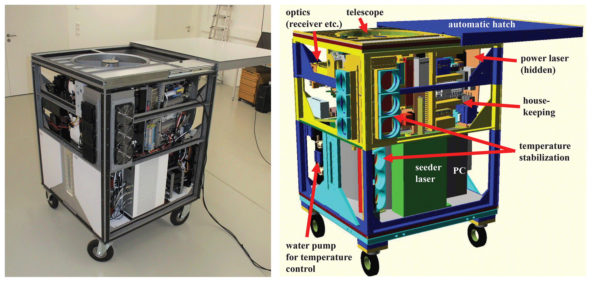
Figure 1Photo and technical drawing of a lidar being used for VAHCOLI. Some important parts can be recognized, such as the telescope, the seeder laser, and the PC. Temperature control and stabilization (different for different sections) are realized using air ventilation and a water cooling system. The dimensions of a VAHCOLI unit (without the wheels and with closed hatch) are 96 cm × 96 cm × 110 cm (length × width × height). The weight is approximately 400 kg, and the power consumption is 500 W under full operation.
2.1.1 Spectral characteristics of scattered signals and lidar components
The lidars being used for the VAHCOLI concept rely on the careful consideration and measurement of various spectral characteristics of laser frequencies, spectral filters, and backscattered light. We therefore briefly recollect the spectral features of the main scattering processes and instrumental components involved (see Fig. 2). The spectral line width (FWHM: full width of half-maximum) of the Doppler-broadened line due to scattering on molecules (Rayleigh) is typically Δνm∼ 1500 MHz (for λ = 770 nm, the potassium resonance wavelength currently being used), which is given by the Maxwell–Boltzmann velocity distribution. The line width is proportional to , so it can be used to measure atmospheric temperatures (T is temperature; mm is the mean mass of an air molecule). The line widths of resonance lines of metal atoms are again given by the Doppler broadening and the broadening due to atomic physics processes such as natural lifetime and hyperfine structure. For potassium, the FWHM is approximately 1000 MHz (von Zahn and Höffner, 1996). The line width of scattered light caused by aerosols is much smaller since aerosols are much heavier than molecules. Stratospheric aerosol particles have radii on the order of 0.1μm, which corresponds to a mass of roughly 7 × 10⁻⁶ ng. This is a factor of ∼ 1.5 × 10⁸ larger than the mass of an air molecule. Therefore, the spectral width of the aerosol signal Δνa is roughly 100 kHz for Δνm = 1500 MHz. The Doppler shift, dν, of the backscattered signal due to background winds is , which allows for measuring line-of-sight winds (νo: laser frequency, v: background wind, c: speed of light). For a laser wavelength of λo=770 nm (νo=389.28 THz) considering Rayleigh or Mie scattering, this shift is dν=2.6 MHz for a wind speed of v=1 m s−1. We also need to take into account the spectral widths of the instrumental components (discussed later), namely the spectral widths of the diode-pumped alexandrite laser (∼ 3.3 MHz) and the high-resolution spectral filter (“confocal etalon”) in the receiver system (approximately 7.5 MHz). For comparison, the Fourier transform width of a laser pulse with a length of 1000 m (100, 1 m) is roughly 60 kHz (600 kHz, 60 MHz). According to their spectral characteristics, the scattering mechanisms mentioned above are used to measure temperatures and winds from Rayleigh scattering (“Doppler-Rayleigh”), temperatures and winds (plus metal number densities) from resonance scattering (“Doppler-resonance”), and winds (plus aerosol densities) from Mie scattering (“Doppler-Mie”).
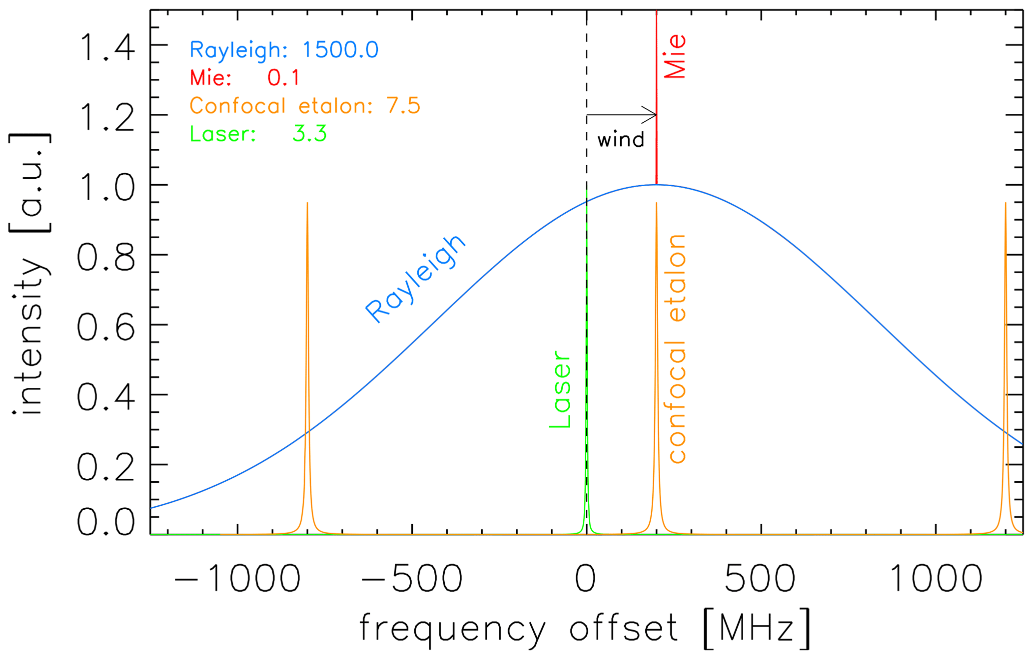
Figure 2Schematic of typical spectral widths (FWHM) relevant for VAHCOLI. The spectral widths (MHz) are given in the insert. Blue: Doppler-broadened Rayleigh signal (same order of magnitude for resonance scattering), red: Mie scattering by aerosols, green: spectrum of the power laser, orange: spectrum of the confocal etalon (free spectral range: 1000 MHz), in this case centered at the Mie peak. Doppler shifting by background winds leads to a shift of approximately 2.6 MHz for a wind of 1 m s−1.
2.1.2 General lidar setup
A key idea behind the lidars being used for VAHCOLI is that all relevant frequencies and spectra (e.g., seeder laser, power laser, backscattered light from the atmosphere, narrowband filter, reference spectrum) are controlled and measured with high precision (discussed later). The atmospheric signal and laser parameters are measured (or actively controlled for the latter) for every single laser pulse. This allows us, for example, to measure the widths and shifts of the spectrally broadened lines while simultaneously determining the spectral characteristics of the receiver in the time between two laser pulses. Narrowband spectral filtering and a small field of view are used to reduce the background, which allows us to use high repetition frequencies and comparatively low-power laser energies. The laser can be tuned to any given frequency within a large frequency range, and spectra are observed at these mean frequencies in great detail. This provides the opportunity to measure the signals from Rayleigh and Mie scattering separately (see Sect. 3).
The frequency of the power laser is controlled by a so-called seeder laser. The seeder laser is used (i) to control the frequency of the power laser and (ii) to measure the spectral specifications of the entire optical path in the receiver system (including the filter characteristics of the etalons) immediately before these filters are used to measure the spectrally broadened and shifted backscattered signal from the atmosphere (Rayleigh, Mie, or resonance).
The seeder laser, the power laser, and the signal from the atmosphere are fed into a receiver system (see Fig. 3), which consists of various optical components such as an interference filter (to block a large part of the solar background spectrum not wanted), a broadband solid etalon with an FWHM close to the Doppler width of the atmospheric molecular line, and a narrowband confocal etalon (FWHM ∼ 7.5 MHz). The largest part of the incoming light is reflected by the confocal etalon, which creates a signal at the detector, DR-R, whereas a small part is transmitted and measured by the detector DMie (see Fig. 3). The frequency of the seeder laser is tuned up and then tuned down again. The amplitude of this tuning is, for example, 2000 MHz in order to cover the Doppler broadened Rayleigh signal. The seeder is used to control the frequency of the power laser for every single pulse, i.e., every 2 ms. The spectral characteristics of the seeder laser, e.g., the frequency as a function of time during tuning up and down, are known precisely due to comparison with a high-resolution Doppler-free polarization spectrum of potassium, which also serves as an absolute frequency reference in the case of resonance scattering for potassium. The parameters controlling the seeder frequencies can easily be adjusted by software according to the scientific requirements. The lidar parameters, e.g., the range of the frequency scan, can be optimized for the measurement of Doppler winds on aerosols, for resonance temperatures, or for a simultaneous observation of Rayleigh, Mie, and resonance scattering. The chopper shown in Fig. 3 helps to separate backscattered light from the middle atmosphere from other sources, e.g., stray light within VAHCOLI. The rotation speed of the chopper and the open segments within the chopper are chosen to effectively open the detectors for atmospheric light at an altitude above 3 km and to allow for the firing of 500 laser pulses per second. The opening of the chopper is synchronized to the firing of the power laser.
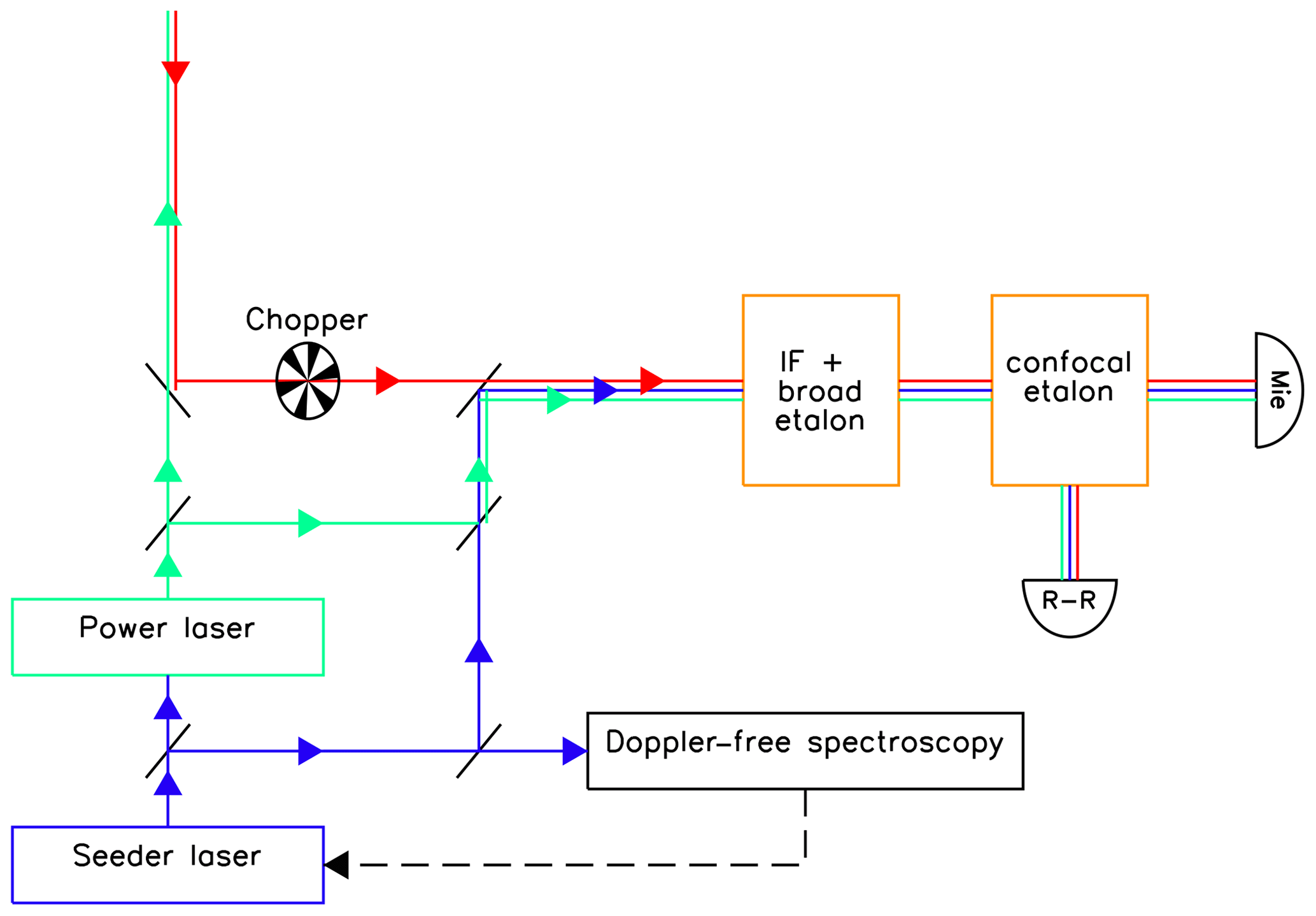
Figure 3Sketch of a lidar being used for VAHCOLI. The frequency of the power laser (green) is controlled by a seeder laser (blue), which itself is controlled by high-precision Doppler-free spectroscopy. When the chopper is open, the signal from the atmosphere (red) is fed into the receiver system, which consists of a broadband interference filter (IF Δν=150 GHz), a broadband etalon (Δν=1000 MHz), a narrowband confocal etalon (Δν=7.5 MHz), and detectors for the Rayleigh or resonance (“R-R”) and Mie channels. When the chopper is closed, parts of the seeder and power lasers are fed into the receiver system to measure their frequencies (see text for more details).
The frequency of the power laser is nearly identical to the frequency of the seeder laser because of a novel cavity control technology called advanced ramp and fire (ARF). A precursor version of this technology has been used since 1998 for the flashlamp-pumped alexandrite ring laser at IAP and later also for an Nd:YAG laser (Nicklaus et al., 2007). ARF allows for control of the mean frequency shift between the seeder and the power laser, and it is not limited to a single laser frequency. This allows for a fast tuning of the power laser over a wide range of frequencies from one pulse to the other. We currently use a maximum tuning rate of 1000 MHz ms−1, which can be increased if required. An example of controlling and measuring the power laser frequency is shown in Fig. 4. The seeder laser (and thereby the power laser) is tuned across the confocal etalon; the frequency range of the tuning (100 MHz) was chosen such that it covers the spectral width of the confocal etalon. The frequency sampling covers frequencies with a difference of 2 MHz, as can be seen in Fig. 4. The advanced ramp-and-fire technique ensures that the frequencies of the power laser pulses are indeed very close to the nominal frequencies, νi (within less than 100 kHz), namely within the width of each red line in Fig. 4. The intensity distribution as a function of νi is given by the convolution of the spectral width of the confocal etalon and the spectral width of the power laser (the spectral width of the seeder laser is only ∼ 100 kHz and can be ignored in this context). Figure 4 demonstrates that the frequency control of the power laser by the seeder laser works very successfully, namely within less than approximately 100 kHz.
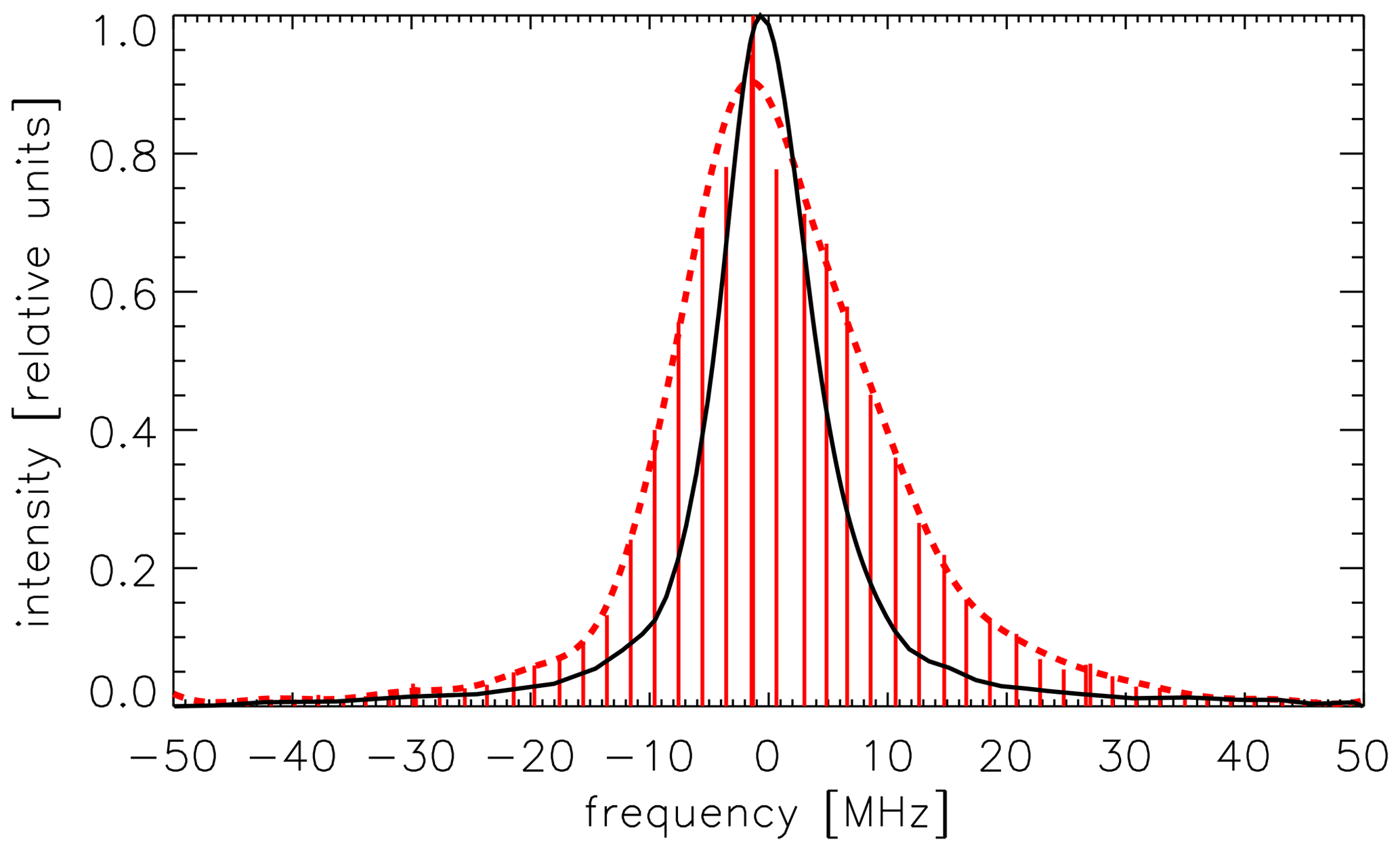
Figure 4Measurement of the convolution of the spectra of the power laser (FWHM ∼ 3.3 MHz) and the confocal etalon (FWHM ∼ 7.5 MHz) taken for a period of ∼ 5 min (150 000 pulses) during first-light operation in January 2020. The power laser is tuned over the spectrum of the confocal etalon; a total of 50 individual mean frequencies of the power laser with a difference of 2 MHz each are chosen (vertical red lines). The power laser matches the requested mean frequencies to better than ∼ 100 kHz, which is within the thickness of the red lines. The dashed red line is an approximate envelope of the vertical red lines. The black line is the spectrum of the confocal etalon measured separately by tuning the seeder laser over the spectrum of the confocal etalon. The slightly asymmetric shape of the red dashed line is a result of a non-perfect optical alignment.
The temporal stability of the laser frequency control is demonstrated in Fig. 5 where measurements of the frequencies of the seeder laser and the confocal etalon are shown. More precisely, in the upper panel the difference between the nominal seeder laser frequency and the actual true frequency is shown; the latter is determined by comparison with high-precision Doppler-free spectroscopy (DFS). The individual peaks of the Doppler-free spectrum serve as an absolute frequency calibration for the seeder laser, which is tuned up and down in frequency and fed into the DFS system. Thereby, the seeder laser frequency is known precisely (within a few kHz) as a function of time and is subsequently used to control the frequency of the power laser. The seeder laser also serves as a reference to lock a transmission peak of the confocal etalon. Note that this procedure implies that (different to other lidar systems) we do not lock the frequency of the seeder laser (nor the power laser) to a single frequency.
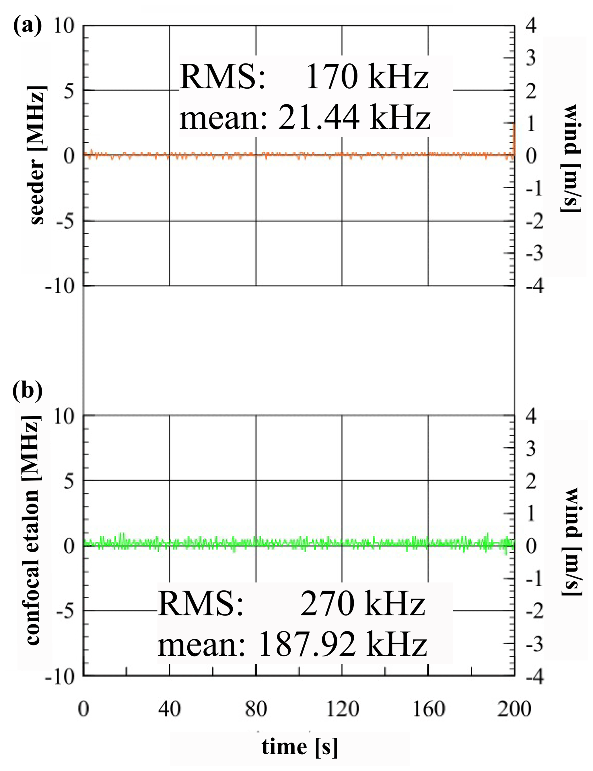
Figure 5(a) Frequency of the seeder laser determined with a time resolution of s. More precisely, the differences between the nominal frequency and the actual frequencies are shown; the latter are determined by comparing with high-precision Doppler-free spectroscopy. Note that the seeder was tuned up and down within a range of 100 MHz, and several scans are averaged within a time period of s. The mean of the frequency difference is 21.44 kHz, and the root mean square (rms) of the fluctuations is 170 kHz. (b) The same but for the confocal etalon. The seeder laser from the upper panel is fed into the confocal etalon, and the nominal frequency is compared to the actual (seeder laser) frequency. The mean of the frequency difference is 187.92 kHz, and the rms of the fluctuations is 270 kHz. For comparison, note that a wind speed of 0.1 m s−1 corresponds to a frequency shift of 260 kHz.
Data points in Fig. 5 are shown for ∼ 3 min with a temporal resolution of s. The mean offset between nominal and true frequencies is only 21.44 kHz, with a root mean square (rms) variation of 170 kHz. The same procedure is repeated for the confocal etalon (lower panel in Fig. 5); i.e., the seeder laser is directed into the confocal etalon, and the nominal and “true” frequencies (from the seeder laser) are compared with each other. The mean uncertainty of the confocal etalon frequency is 187.92 kHz, which corresponds to an uncertainty in the wind measurements of 0.072 m s−1. In fact, the final contribution of this uncertainty to the wind error is even smaller since the offset (in this case 187.92 kHz) is measured and later considered in the data reduction procedure.
Finally, the spectrum received from the atmosphere is compared with the spectral characteristic of the instrument, including the laser line width and spectral filters. For Rayleigh and Mie scattering it is not necessary to know the absolute frequency of the laser light or the absolute frequency position of the etalon's transmission function. It is only important to know the frequency of the pulsed laser relative to the frequency of the spectral filters which is achieved by the procedure described above. On the other hand, resonance scattering requires frequency measurements on an absolute frequency scale, which is achieved by applying Doppler-free polarization spectroscopy to an atomic absorption line of potassium; this, in turn, is used to control the output of the seeder laser and the spectral filters with an accuracy of a few kilohertz (kHz; see above).
2.2 Laser specifications
A VAHCOLI unit requires a compact, efficient, and high-performance laser designed for atmospheric applications. For Doppler-Mie the laser should preferentially have an exceptionally small line width. For Doppler-resonance the laser must be tunable to an atomic absorption line. We have developed a highly efficient, narrowband, diode-pumped alexandrite ring laser in cooperation with the Fraunhofer Institute for Laser Technology in Aachen (Höffner et al., 2018; Strotkamp et al., 2019). The laser head includes various subsystems such as a Q-switch driver, cavity control, power measurement, and a beam expansion telescope, all of which are placed in a sealed housing for touch-free operation over long periods. The laser head is pumped via a fiber cable connected to a separate diode array which acts as an optical pump. The beam profile of the laser is nearly perfect with very little aberration (M2=1.1). The spectral width is ∼ 3.3 MHz with a pulse length of ∼ 780 ns. In Q-switch mode, the variation of the output power from pulse to pulse is only 0.2 %. A first test of the robustness of the laser was performed when it was transported from Aachen to Kühlungsborn in early 2020. After a transport of nearly 700 km in a standard truck the laser performed without any degradation (see Sect. 3). Thereafter, the entire lidar was aligned and operated successfully during a 6-week period without any further adjustment.
2.3 Telescope and receiver
The field of view (FOV) of the telescope is currently 33 µrad, which corresponds to a diameter of 3.3 m at a distance of 100 km. The accuracy to keep the laser beam inside the field of view of the telescope is better than 10 cm at 100 km, which corresponds to a position accuracy of better than 1 µrad. This is achieved as follows: once the outgoing laser beam and the optical axis of the telescope are co-aligned, the photons being scattered by 180∘ from the atmosphere follow the optical path of the outgoing laser beam but in the retrograde direction and thereby arrive at the detectors. The light from the atmosphere is separated from the outgoing laser pulse using its polarization characteristics. The compact design of the lidar ensures that the alignment between the laser beam and the telescope is preserved on short timescales, i.e., no active control of the outgoing laser beam on a pulse-to-pulse basis is needed. Slow drifts of the laser beam relative to the optical axis of the telescope caused by, for example, temperature drifts are compensated for by a control loop (maximizing the atmospheric signal) with a time constant of a few minutes. The current plan is to have five telescopes with different viewing directions which are fed subsequently (switching within 1 ms) by one laser. Only one receiver system (and one transmitter) will be needed.
The prime mirror (diameter: 50 cm) and related optics are integrated into a system which is manufactured by large-scale 3D printing. Complex thermal balancing considerations ensure that the telescope (optics and walls) are stabilized to the outside temperature by maintaining an active airflow through the cube. This prevents convection and turbulence and also keeps dust, snow, and sea salt away from the optics. The mechanical structures supporting the primary and secondary mirrors are stabilized to the temperature inside the main housing. This eliminates the need to realign the telescope when ambient temperatures change, for example, from day to night. In summary, the mechanical design and thermal balancing allow us to operate the lidar under harsh conditions in a wide range of ambient temperatures during both day and night.
The most important components of the receiver system are the spectral filters in combination with other optical systems such as the seeder laser and the Doppler-free spectroscopy (see Fig. 3). All components fit inside a compact, optically tight, dust-free, and lightweight housing of 15 × 15 × 80 cm3, which is manufactured by 3D printing together with all mechanical mounts for the optical components (∼ 75 in total). Avalanche photodiodes (APDs) are used for counting photons.
2.4 Data acquisition and lidar control
After a laser pulse has been released, it takes 1 ms until photons scattered at a distance of 150 km arrive at the detector. This implies that the maximum possible pulse repetition frequency is kmax = 1000 laser pulses per second (we use 500 s−1), assuming that only one laser pulse is in the air at any given time. Photons from a single pulse scattered from a height range δz arrive at the detector in a time interval of . The number of photons Nph arriving from the height range δz create a count rate Rsgl at the detector of . Here and in the following we ignore any impact by the dead time of the detector. The time between two pulses is given as , where k is the pulse repetition frequency. Therefore, the effective number of photons counted per time interval is reduced relative to Rsgl by a factor of . For example, for δz=200 m and k=500 s−1 the reduction factor is . In other words, the number of photons, Nph, counted per integration time δt and height interval δz is related to the count rate (R) and the pulse repetition rate (k) via
For technical reasons the count rate of typical detectors (PMT, APD) is limited to approximately Rmax = 107 Hz. As mentioned before, the maximum pulse repetition rate is given by the uppermost altitude (zmax) wanted: kmax = 1000 s−1 for zmax = 150 km. Higher pulse repetition frequencies may be chosen if the maximum altitude is reduced. According to Eq. (1) this leads to a larger number of photons at a given altitude. The receiver relies on a high-speed single-photon data acquisition system with compression for fast analysis. Each pulse is stored with 1 m altitude resolution and with further information regarding, for example, pulse energy as well as the frequency and FWHM of the laser pulse. Each VAHCOLI unit is connected to the internet and, if necessary, can be controlled and operated in real time. This includes the frequency control of the seeder and power lasers as well as the filter system (see above). The entire receiver system (actually the entire lidar) is based on a single standard PC with integrated commercially available electronics. Data from the lidar are automatically downloaded to a remote server.
2.5 Measuring principle
2.5.1 Temperatures and winds from Rayleigh and resonance scattering
A standard method to derive temperature profiles from measured altitude profiles of number densities is based on the (downward) integration of the hydrostatic equilibrium equation. Since only relative number densities are relevant here, the lidar count rates from Rayleigh scattering can be applied after taking into account the square of the distance (lidar equation). Some uncertainties are introduced by the unknown temperature at the top of the profile (also called “start temperature”), which, however, decrease exponentially with altitude. A more detailed error analysis for Rayleigh temperatures is presented in Sect. 4.2. Note that narrowband spectral filtering allows us to separate the Rayleigh signal from the Mie signal (see below). This implies that Rayleigh temperatures can be derived even in the presence of aerosols. Since the spectral width of the Rayleigh signal is proportional to it can also be used to measure temperatures. This is planned for the future, together with a comparison of temperatures from integration (hydrostatic equilibrium equation).
Line-of-sight winds are measured by lidars by detecting the spectral shift of the backscattered light: Rayleigh, resonance, or Mie. This is rather challenging since this shift is normally small compared to the spectral width of the backscattered signal. Various techniques have been developed to measure the spectral shift, e.g., employing double-edge or single-edge or vapor filters (see, for example, Chanin et al., 1989; She and Yu, 1994; Baumgarten, 2010). In our first measurements presented in Sect. 3 we concentrated on measuring winds by detecting the spectral shift of the narrowband aerosol signal.
Resonance scattering on metal atoms (K, Fe, Na) has frequently been applied to derive metal atom number densities and temperatures in the altitude range of roughly 80 to 120 km by measuring the Doppler width of the backscattered light (see, for example, Fricke and von Zahn, 1985; von Zahn et al., 1988; Alpers et al., 1990; She et al., 1990; Clemesha, 1995; Höffner and Lautenbach, 2009; Chu et al., 2011). Unlike these other lidars, VAHCOLI can observe line-of-sight winds and temperatures from resonance scattering in the presence of aerosols, namely NLC. The resonance scattering application of VAHCOLI is based on our experience with a potassium lidar being operated at several locations, for example on the research vessel Polarstern and in Spitsbergen (Höffner and von Zahn, 1995; von Zahn and Höffner, 1996; Lübken et al., 2004; Höffner and Lübken, 2007). The technique has been improved substantially for a VAHCOLI unit by applying high-temporal- and high-spectral-resolution detection of Doppler broadening (temperatures) and Doppler shift (line-of-sight winds). See Sect. 2.1.1 for more details.
2.5.2 Aerosol parameters and winds
VAHCOLI is also designed to measure the presence of aerosols, more precisely background aerosols, polar stratospheric clouds (PSCs), and noctilucent clouds (NLCs). Precise and fast measurements of the spectrum of the filters allows for positioning the narrowband spectral filter (a few MHz) exactly at the position of the Mie peak which corresponds to aerosol backscattering, as is shown in Fig. 2. Since the Mie spectrum in the stratosphere is also very narrow (typically 0.1 MHz; see above) only the backscattered signal from aerosols is detected, whereas nearly all of the Rayleigh scattering is blocked (this also means that the solar background signal is negligible, which is known as “solar blind”). Therefore, Mie scattering is detected irrespective of the Rayleigh signal and vice versa. The precise measurement of these spectra allows us to derive line-of-sight winds from the Doppler shift of the Mie peak (see Sect. 3). In the future, we envisage making multi-color observations of PSCs and NLCs to deduce particle characteristics such as size and number densities (see, for example, von Cossart et al., 1999; Alpers et al., 2000; Baumgarten et al., 2010).
2.5.3 Metal densities
Resonance scattering on metal atoms in the upper mesosphere–lower thermosphere is applied to derive metal number density profiles. We have used this technique mainly to observe potassium (λ = 770 nm) and iron (λ = 386 nm), but other metals have also been measured (see, e.g., von Zahn et al., 1988; Gerding et al., 2000; Chu et al., 2011). The capability of VAHCOLI to measure vertical and horizontal structures in metal densities allows us to address several open science questions regarding the causes of the observed temporal and spatial variability (see Sect. 5.5). The current version of the VAHCOLI units is designed to detect potassium atoms. In the future we envisage developing new and compact lasers and/or frequency doubling techniques to measure other species, including iron and sodium.
2.5.4 Other
Several secondary parameters are typically derived from the prime observables such as the potential (Epot) and kinetic energy (Ekin), momentum flux, and wave action densities. Note that the latter requires us to measure the background mean winds in order to consider the Doppler shifting effect on gravity waves. A Helmholtz decomposition of the flow, i.e., its divergent and rotational component, can be applied to better understand the physical processes involved. Lidars typically measure relative number densities, n(z), which allows for the determination of Epot from
i.e., from number density instead of temperature fluctuations. Using number densities allows us to reach higher altitudes and avoids uncertainties due to the start temperature.
Since VAHCOLI measures the dynamical and thermal components of the flow field, the heat flux due to fluctuations caused by gravity waves can also be derived. Statistical quantities can be derived from fluctuations: for example, longitudinal and transversal structure functions.
2.6 Lidar operation
After manufacturing, installation, and testing in the laboratory, the lidar shall be transported to a location of interest where it is assembled for operation under field campaign conditions. The lidar is designed as a sealed and automated system which is controlled remotely and can run for long periods without any manual intervention. The autonomous operation includes the ability to stop measurements on short notice and very quickly (from one pulse to another) if required by, for example, air safety regulations or by bad weather conditions. Information regarding air safety is currently provided by an internal camera, and weather conditions are monitored by an external weather station. Further constraints provided by external sources, e.g., a weather radar or air traffic control, can easily be incorporated into the lidar operation. If conditions are favorable again, the lidar switches on automatically within less than 1 min.
In the following section we show results from the very first atmospheric measurements by a prototype of a VAHCOLI unit (“first light”), which were made over the period of 17 to 19 January 2020 at the IAP in Kühlungsborn (54∘ N,12∘ E). Some specifications of this lidar are summarized in Table 1. In Fig. 6 we show raw count rates observed on 19 January 2020 by the detectors DR-R and DMie (see Fig. 3). The goal of these measurements was to perform a first test of the entire lidar, i.e., laser, frequency control and analysis, telescope, detection system, Doppler-free spectroscopy, and lidar operation, under realistic conditions including rain, low temperatures, and storms without touching the system for several days. Note that the FOV of the telescope was only 33μrad, which allowed measurements even during full daylight. According to the description of the lidar presented in Sect. 2.1.2 the confocal etalon is stabilized to a certain frequency, νcf, and the power laser is normally tuned by typically ±1000 MHz relative to this frequency. In the first measurements presented here we concentrated on wind measurements (Doppler-Mie) and have therefore used a much smaller frequency range for tuning, namely only ±50 MHz. In the case shown in Fig. 6, the etalon's central frequency, νcf, was chosen such that it coincides with the mean resonance frequency of potassium to allow for a detection of the potassium layer. The etalon transmits backscattered light from the atmosphere within a frequency range of νcf±Δνcf, where Δνcf = FWHM/2 and FWHM ∼ 7.5 MHz (blue line in Fig. 6). Note that the spectral width of the Mie peak is only ∼ 0.1 MHz, which can be neglected in this context. Furthermore, Δνcf is much smaller than the spectral width of the Doppler-broadened Rayleigh signal; i.e., only a very small fraction of the backscattered light from the atmosphere passes through the etalon, and the rest is reflected and detected by a separate detector (red line in Fig. 6).
Table 1Specifications of the prototype lidar used for the first measurements in January 2020 at the IAP in Kühlungsborn (54∘ N, 12∘ E).
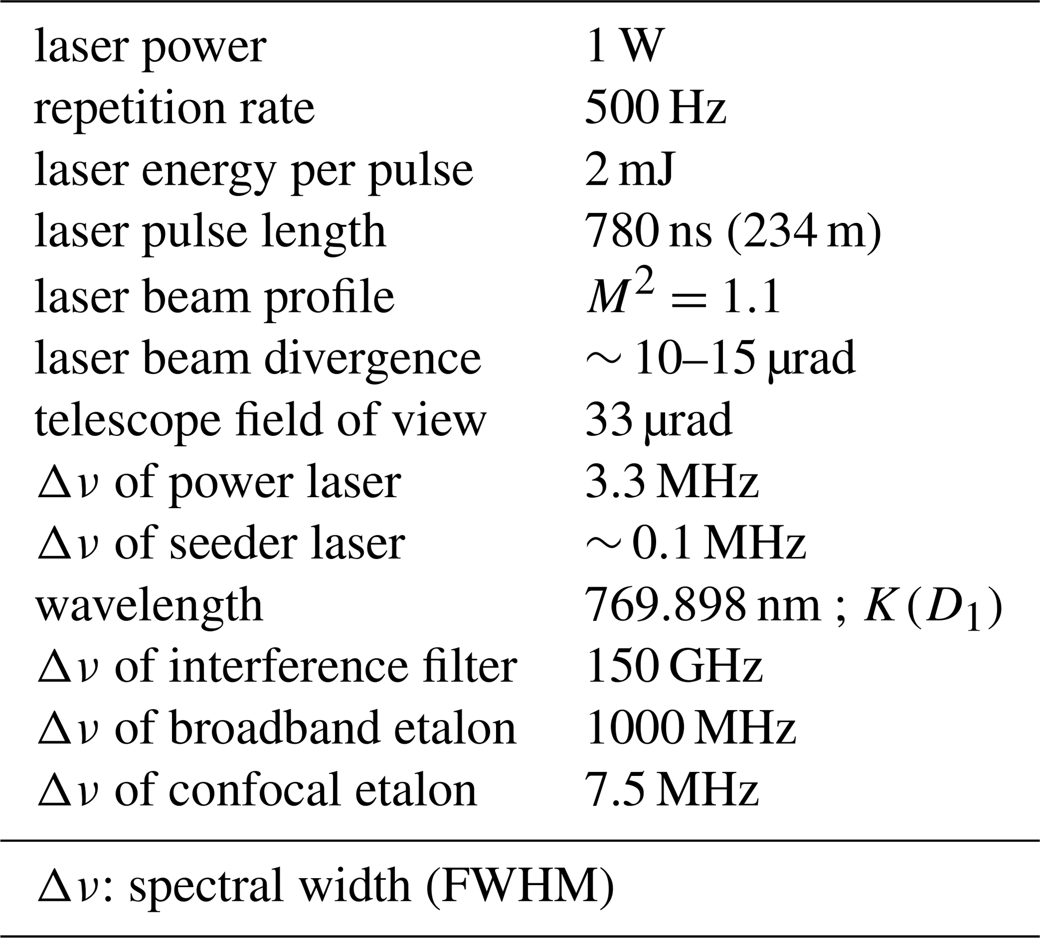
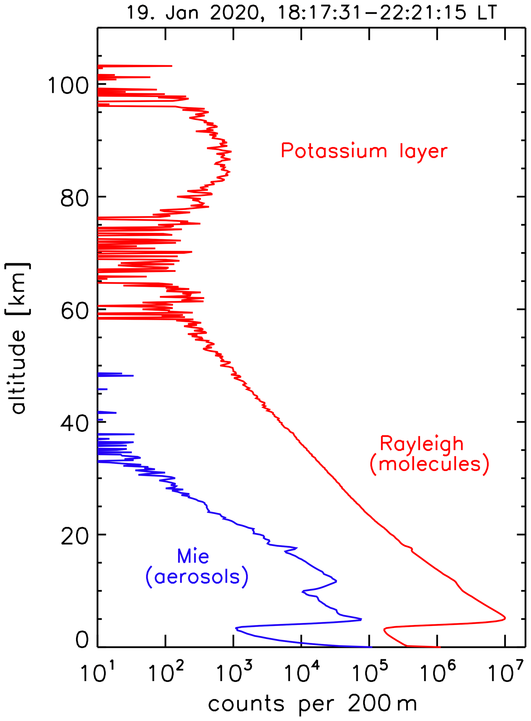
Figure 6Altitude profiles of raw backscattered signals (“first light”) observed by the detectors DR-R and DMie on 19 January 2020 at 18:17:31–22:21:15 LT at the IAP in Kühlungsborn (see Fig. 3). Red line (DR-R): mainly Rayleigh scattering on molecules (below ∼ 70 km) and resonance scattering on potassium atoms (∼ 75–100 km). Blue (DMie): Mie scattering on stratospheric aerosols. Below ∼ 30 km the signal at DR-R includes a very small contribution from Mie scattering, which is subtracted during further processing (see text for more details). The decrease in the signals below approximately 5 km is caused by the chopper blocking the atmospheric signal.
At altitudes below the potassium layer the total signal is due to backscattering from molecules (Rayleigh scattering) and a small contribution from Mie scattering from aerosols at altitudes below ∼ 30 km. When the frequency of the Mie peak is outside the frequency range of the confocal etalon, νcf±Δνcf, the backscattered light from the atmosphere detected at DMie stems from Rayleigh scattering only, whereas DR-R detects Rayleigh (and resonance) scattering plus a small contribution from Mie scattering. The signal at DR-R is much larger compared to DMie since most of the signal is reflected by the narrowband confocal etalon (see Figs. 2 and 3). When the power laser frequency is within νcf±Δνcf, however, the signal at DMie includes Mie scattering, which varies when scanning the power laser, whereas the contribution from Rayleigh scattering is basically constant within νcf±Δνcf because the Rayleigh peak is very flat within the frequency range νcf±Δνcf. The signal at DMie can therefore be used to measure Mie scattering only, which is subsequently used to subtract the Mie signal from the Rayleigh signal. Furthermore, the signal at DMie is used to derive the Doppler shift of the Mie peak due to winds. In Fig. 6 we show signals from the detectors DR-R and DMie. The exponential decrease in the Rayleigh signal and some very small “bumps” due to aerosol scattering are clearly visible. After subtracting the Mie contribution the signal can be used to determine a temperature profile (not shown). Note that temperatures can also be derived from the spectral width of the Rayleigh signal (not done in this first test). The Mie signal caused by stratospheric aerosols is roughly 0.1 %–10 % of the Rayleigh signal and disappears above roughly 30 km.
In Fig. 7 we show line-of-sight winds derived from the Doppler shift of the Mie peak observed on 19 January with a height resolution of 200 m, integrated for a period of 20 min (18:10:00–18:30:00 LT). As can be seen from this figure, the central frequency of the spectra changes with height, which is used to calculate line-of-sight winds. Note that wind uncertainties shown in the right panel of Fig. 7 deviate substantially from our estimates presented later (see Sect. 4.1) because the actual aerosol distribution was rather different and the lidar performance was not yet optimized. We compare these winds to the ECMWF (European Centre for Medium-Range Weather Forecasts) profiles which are closest in time and space (horizontal resolution: ∼ 9 km). The height resolutions of ECMWF winds are approximately 250 and 600 m at 5 and 25 km, respectively. Here we have assumed somewhat arbitrarily that the lidar picks up 4 % of the meridional winds corresponding to an off-zenith tilt of the laser beam by 2.3∘. This is certainly realistic when considering that no attempt has been made during this first test to precisely align the laser beam to the vertical. In the future the telescope pointing will be measured with high accuracy by an integrated sensor.
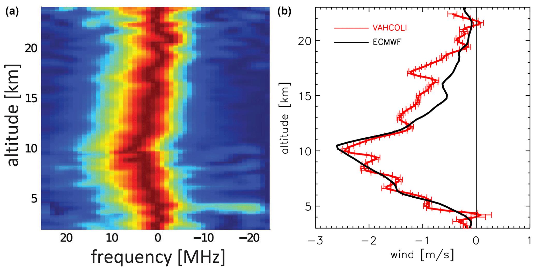
Figure 7Wind profiles from a prototype of a VAHCOLI unit as derived from the Doppler shift of the Mie signal measured at the IAP in Kühlungsborn. (a) Spectra of the Mie signal (relative to the mean frequency νo) as a function of altitude. The shift of the spectra relative to νo is used to derive line-of-sight winds. (b) Observed line-of-sight wind profile (red line and error bars) with a height resolution of 200 m, integrated in the time period 18:10:00–18:30:00 LT on 19 January 2020. Black line: ECMWF wind profile closest in time and space. A small fraction (4 %) of ECMWF meridional winds has been added to ECMWF vertical winds assuming that the lidar has a small tilt relative to the vertical by 2.3∘. See text for more details.
The agreement between the observations and ECMWF winds is very good considering the constraints regarding temporal–spatial coverage and sampling. The fact that this was the very first test of the entire lidar system, while using some preliminary optics, is very encouraging. The results shown in Fig. 7 demonstrate that the initial optical alignment of the lidar, including laser beam adjustment relative to the telescope, was stable under harsh conditions and no realignment was required. The performance of the lidar during this first-light measurement does not reflect the full potential of the system. We expect significant improvements once the telescope and detector systems are optimized. As will be explained in more detail in Sect. 6, the efficiency of VAHCOLI units will be improved further in the near future.
4.1 Expected performance
The following calculations of sensitivities and uncertainties are based on our experience with a potassium lidar, which was housed in a container and operated at various remote locations such as the research vessel Polarstern and in Spitsbergen (von Zahn and Höffner, 1996; Höffner and Lübken, 2007). In Fig. 8 we show expected count rates (R) as a function of altitude, which in this case reaches the maximum possible value of Hz at 20 km. We have assumed a laser power of 6 mJ (next generation of this laser) and a detector system efficiency of 30 %. For a typical time and height interval of δt = 5 min and δz=200 m, respectively, and a pulse repetition frequency of k=500 s−1 this gives the number of photons as a function of altitude according to Eq. (1), also shown in Fig. 8. For example, for Hz (at 20 km) the number of photons (at 20 km) in a time and height interval of 5 min and 200 m, respectively, is Nph = 2 × 10⁶. We have also indicated a typical dark count rate of 20 Hz in Fig. 8, which is realistic for state-of-the-art detectors. The green line in Fig. 8 gives the temperature uncertainties according to Eq. (5) (discussed later). The blue lines indicate uncertainty in the wind measurement, which results from the shift of the Rayleigh spectrum (above 20 km) and from the shift of the Mie peak (below approximately 30 km). We have further assumed that at 30 km the Mie signal is 0.5 % of the Rayleigh signal and that the signal increases to 10 % at 10 km. These values are consistent with typical observations of Mie scattering from stratospheric aerosols but may vary substantially throughout the season and from one location to another (Langenbach et al., 2019).
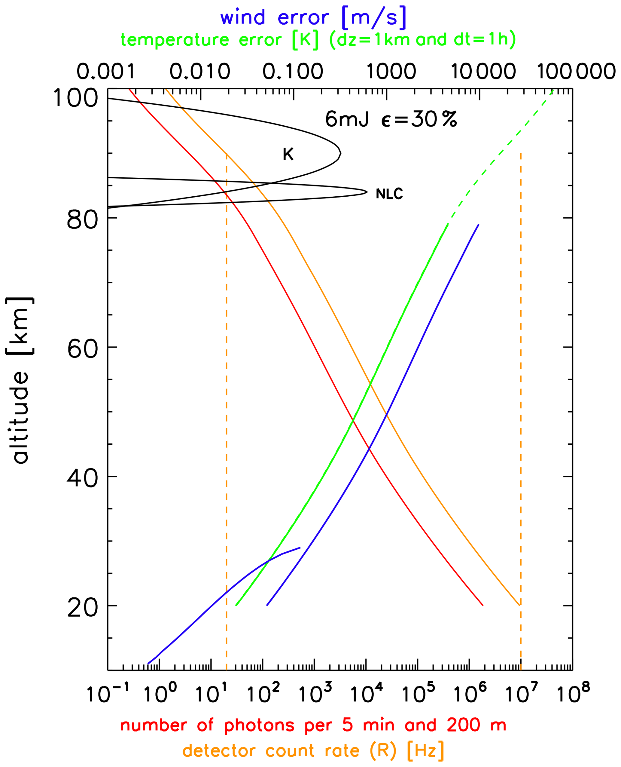
Figure 8Sensitivity of a VAHCOLI unit to measure temperatures, winds, and aerosols. Lower abscissa, orange: count rate; red: number of photons (Nph) per time and height interval of δt = 5 min and δz=200 min, respectively. Nph would increase by a factor of 60 if instead δt = 1 h and δz = 1 km had been chosen. Black lines at 80–100 km: approximate number of photons expected from the K and NLC layers. The vertical dashed orange lines indicate the maximum achievable count rate (107 Hz) and typical dark count rates of the detector (20 Hz). Upper abscissa, green: temperature error for an integration time and altitude bin of δt = 1 h and δz = 1 km, respectively. Blue: error of winds obtained from stratospheric aerosols (Doppler-Mie, lower part) and from Doppler-Rayleigh (upper part). These calculations assume a laser energy of 6 mJ and an overall detection efficiency of 30 %.
The calculation of the wind error is based on our experience that it takes approximately 100 000 photons to measure winds with an accuracy of 1.35 m s−1. Within limits (background noise, etc.) the accuracy is proportional to the square root of the number of photons. As can be seen in Fig. 8, winds can be measured with high precision, i.e., better than 1 m s−1 below 40 km and 10 m s−1 below 70 km, respectively. Due to the small line width, Mie scattering is particularly suitable for measuring winds. In Fig. 8 we also indicate the number of photons expected from an NLC layer assuming a backscatter coefficient at the peak of (see, for example, Fiedler et al., 2009). We also show a typical backscattered signal from a potassium layer with a maximum number density of 50 atoms cm−3.
4.2 Error analysis for Rayleigh temperatures
As is explained above, the lidars being built for VAHCOLI can measure the Rayleigh signal without contamination due to aerosols. We consider altitudes sufficiently below the uppermost height at which uncertainties due to the start temperature are negligible. Starting from an altitude bin centered at z1 with a temperature T1 and number density n1, the following equation gives the temperature error in the next height bin (at z2) due to uncertainties in density measurements Δn1 and Δn2 at levels z1 and z2, respectively:
where n2 is the number density in the altitude bin centered at z2, and Hp is the pressure scale height. This equation can be further simplified by assuming that Hp≈Hn within a height interval of (which is typically a few hundred meters only) and that the uncertainties in ni are determined by Poisson statistics of counting Ni photons, i.e.,
Since N1≈N2 within the height interval δz we finally get
The number of photons counted per time and altitude interval, N(z), decreases with altitude according to
where Nref is the number of photons counted at the reference altitude zref, and Hn is the number density scale height. In Fig. 9 altitude profiles of temperature errors according to Eq. (5) are shown assuming a number of photons at the reference level (20 km) of Nref = 2 × 10⁶ (see above) and Nref = 2 × 10⁵, respectively. Since count rates are normally suppressed at lower altitudes (to avoid a saturation of detectors) they may be increased at higher altitudes, for example, by reducing the attenuation in the receiver. Using telescopes with appropriate diameters is another method to focus on certain altitude ranges. In Fig. 9 we have assumed an enhancement of N due to “cascading” by a factor of 100 (for Nref = 2 × 10⁶) at altitudes above 50 km, which leads to a reduction of ΔT by a factor of 10. In total, typical temperature errors are smaller than 5 K up to the upper mesosphere. Another method to increase the effective count rate is to increase the height range (δz) and/or the integration time (δt). In Fig. 10 the effect of increasing δt and/or δz on temperature errors is shown. More precisely, temperature errors (ΔT) are shown as a function of , where δtref = 5 min and δzref=200 m, and the number of photons at the reference level (zref = 20 km) is Nref = 2 × 10⁶. For example, increasing δz⋅δt by a factor of 60 (e.g., by increasing the integration time from 5 min to 1 h and the height interval from 200 m to 1 km) decreases the temperature error at 50 km from ΔT=5.3 K (g=1) to ΔT=0.7 K (g=60).
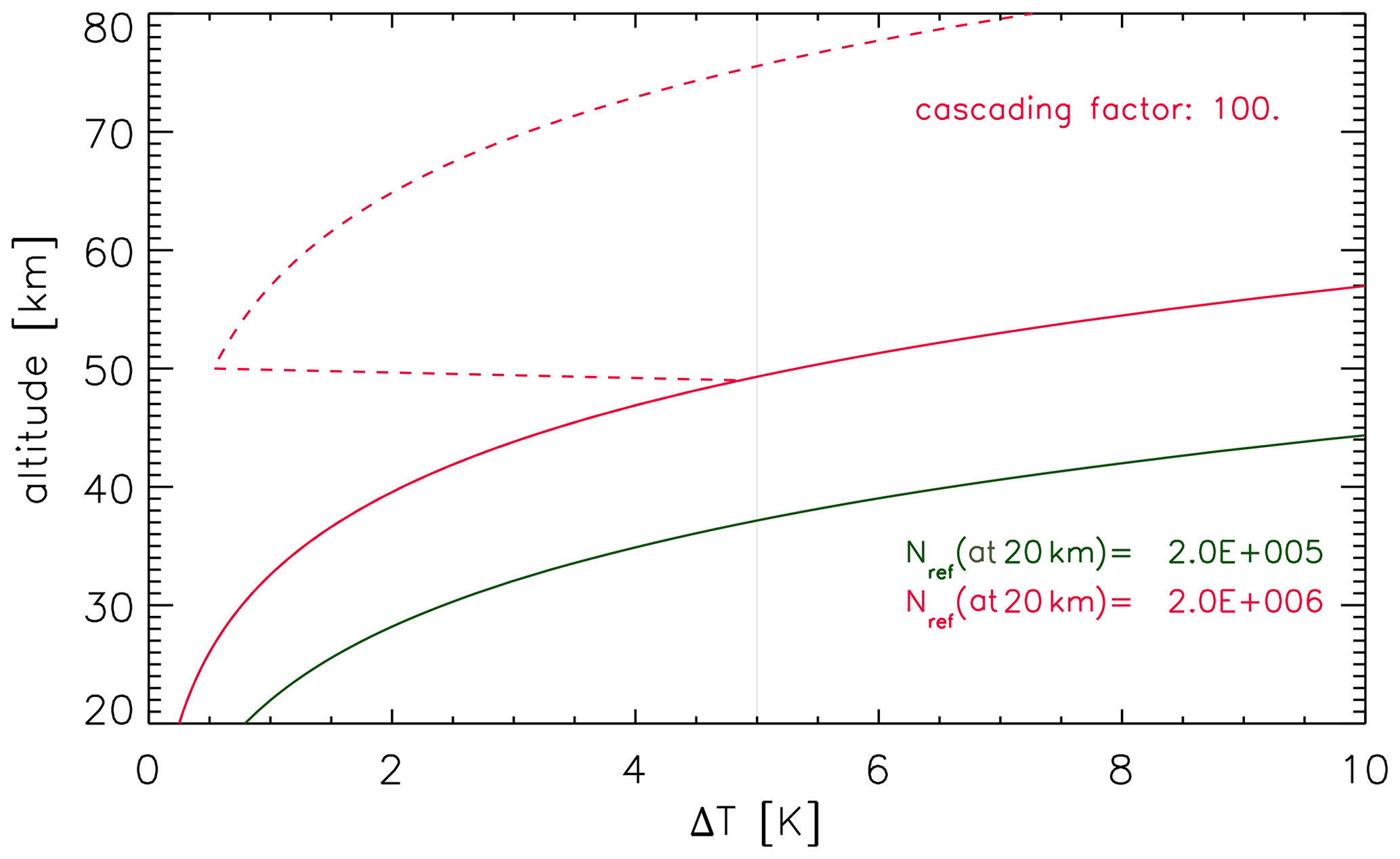
Figure 9Temperature error according to Eq. (5). Here we have assumed that the number of photons counted at an altitude of 20 km per time interval δt = 5 min and height interval δz=200 m is 2 × 10⁶ (red) and 2 × 10⁵ (green), respectively. The dashed red line indicates the effect of cascading the detector by a factor of 100 (see text for more details).
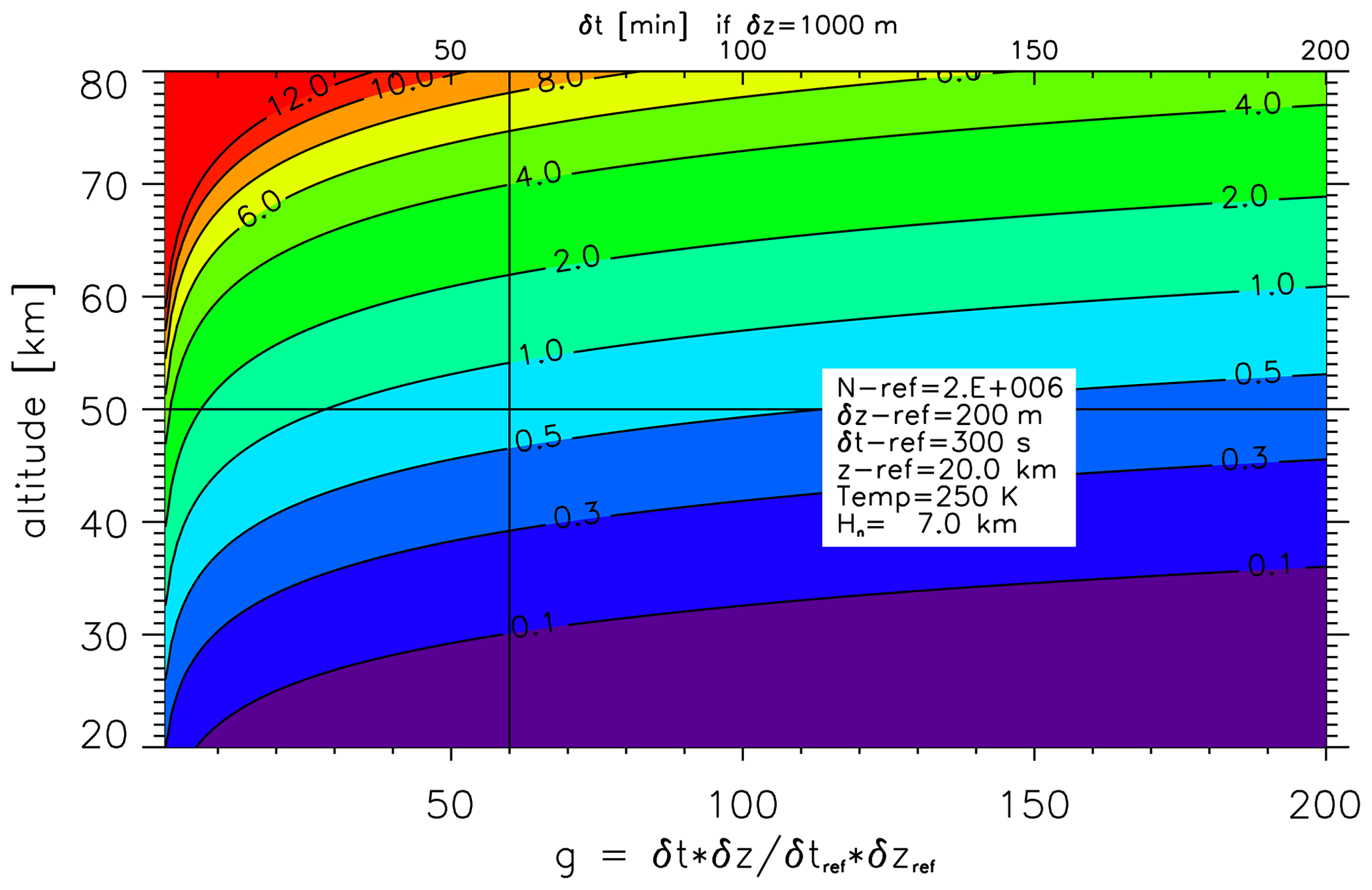
Figure 10Impact of increasing the time (δt) and/or the height interval (δz) on the temperature error from Eq. (5). Temperature errors are shown as a function of , where δtref = 5 min and δzref=200 m. Nref = 2 × 10⁶ is the number of photons at zref = 20 km. The upper abscissa shows the time interval δt in minutes if δz = 1000 m.
4.3 Multi-beam operation and horizontal coverage
The flexibility of VAHCOLI allows us to place the lidars at distances which are optimized according to the science objectives (see below). The current plan is to build four VAHCOLI units (NV=4) with five beams (NB=5) each, with one beam pointing vertically and four beams pointing at a zenith angle of, e.g., χ=35∘ in two orthogonal directions. In Fig. 11 (upper panel) an example of a constellation of four VAHCOLI units with five beams each is shown. At any given altitude there are a total of laser beams available, which gives a total of i=190 combinations of horizontal distances. In the lower panel of Fig. 11 these 190 horizontal distances are shown (abscissa) for a selection of 12 different scenarios (ordinate), including the scenario shown in the upper panel of Fig. 11. Horizonal scales from several kilometers up to hundreds of kilometers are detectable where nearly all directions in the horizontal plane are covered. Even equal horizontal distances contain rather important information since they are located at different places (non-homogeneity) and/or point in different horizontal directions (non-isotropy).
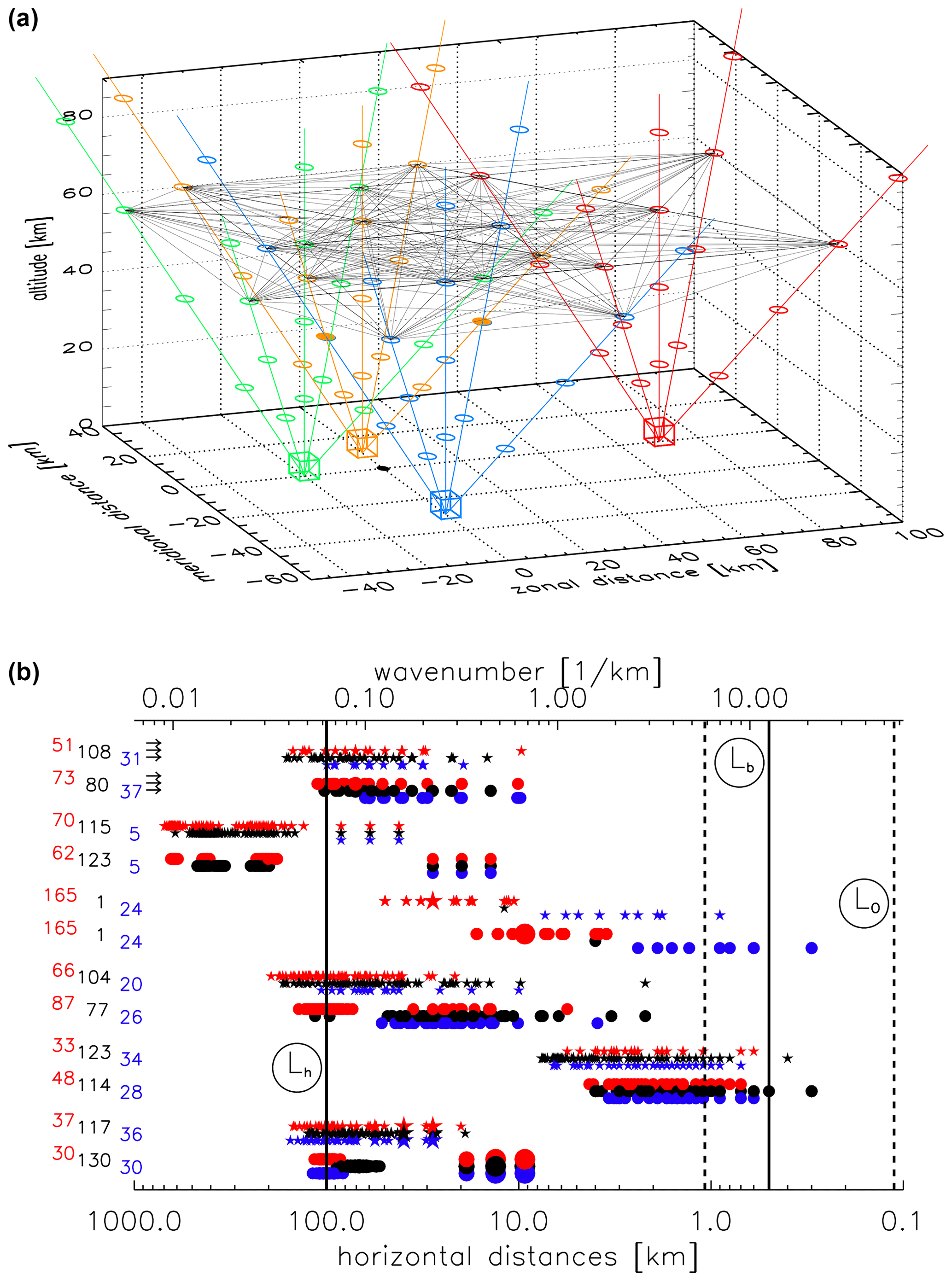
Figure 11Horizontal coverage by VAHCOLI consisting of four units with five beams each. (a) Example of positions of four lidars (with five beams each) located at horizontal positions (x,y) of (, blue), (, green), (, orange), and (, red), all in kilometers. At each location the zenith angles of the five beams are 0, 35, 35, 35, and 35∘. The azimuth angles of the four tilted beams at all four stations are 45, 135, 225, and 315∘. The locations of the beams at certain altitudes, namely 20, 40, 60, and 80 km, are marked by small circles. Thin black lines show all 190 horizontal connections between the circles at 60 km. (b) Horizontal coverage by four lidars with five beams each; the four locations are chosen from various scenarios. Each point gives the horizontal distance between two beams at an altitude of 20 km (circles) or 60 km (stars). The size of the symbols indicates that several identical distances are represented. The colors indicate the azimuth of these connections. Red: east–west (0∘ ± 20∘), blue: north–south (90∘ ± 20∘), black: others. The corresponding numbers of cases are listed on the left ordinate (total of 190). The uppermost scenario (highlighted by small arrows) shows the case presented in the upper panel. The vertical lines indicate scales which are relevant for stratified turbulence (see Sect. 5.3 for more details).
If the beams in all four lidars are aligned equidistantly the maximum horizonal coverage is (, where is the (altitude-dependent) horizonal distance between two beams. For example, for χ=35∘ the horizontal distance between two beams at 50 km is 35.0 km, and the maximum horizontal distance covered by four lidars, which are located at equal horizontal distances, is 385 km. Many other scenarios may be chosen: for example, concentrating on smaller scales by placing the systems very close to each other and choosing a small zenith angle with similar azimuths. On the other hand, several VAHCOLI units may be located at distances of several hundred kilometers to concentrate on processes on synoptic scales. Any combination of such scenarios may be chosen, of course, depending on the availability of lidars and appropriate locations.
5.1 General
Dynamical processes on medium spatial scales (up to several hundred kilometers) are important for the atmospheric energy and momentum budgets, which are directly relevant for climate models on regional and global scales (see, e.g., Becker, 2003; Shepherd, 2014). More specifically, this concerns the question of how energy and momentum are transferred from large to small scales (or vice versa?) and how the horizontal and vertical transport of energy, momentum, and constituents is best described. A prominent example of dynamical impact on the background atmosphere is the summer mesopause region at high latitudes where temperatures deviate by up to 100 K from a state which is controlled by radiation only. This strong deviation is primarily caused by gravity waves, which deposit energy and momentum, resulting in a “residual circulation” and associated upwelling and cooling. Major aspects of this dynamical control of the atmosphere are only poorly understood due to the complexity of the problem from both the experimental and theoretical point of view. In models, the impact of these processes is typically considered by parameterizations. The extent to which these parameterizations adequately describe the real atmosphere can best be assessed by comparing models with observations which are capable of fully characterizing the atmospheric variability at these medium scales. Temporal and spatial variability is observed in the atmosphere over a large range of scales, which reflects various processes and their (mostly) nonlinear interactions. Since these fluctuations vary in time and space it is necessary to measure spatial and temporal variations of, e.g., winds and temperatures simultaneously to achieve a complete picture.
The ultimate aim of VAHCOLI is to characterize the three-dimensional and time-dependent morphology of the atmospheric flow, including gravity waves. This will allows us to disentangle the temporal from spatial variability of the main flow and associated fluxes and to test frequently assumed simplifications in modeling (and some observations) regarding homogeneity, isotropy, and stationarity. In this paper we concentrate on medium scales, i.e., horizontal distances of 1 km to a few hundred kilometers and vertical distances of 100 m to several kilometers.
It is often assumed that atmospheric processes on medium scales are stationary, which is very unlikely to be true in general since energy and momentum are continuously removed from the flow. Whether or not this assumption is perhaps valid within certain limits or within certain scales may be verified by comparing with suitable observations spanning a sufficient range of temporal and spatial scales. Other assumptions include isotropy and homogeneity, for example, regarding fluctuations in the zonal and meridional direction. Again, such similarities are rather unlikely because normally the background flow is systematically different in the zonal compared to the meridional directions.
There are several rather fundamental questions in atmospheric dynamics to which VAHCOLI can contribute for a better understanding. For example, are the governing processes of fluctuations at spatial scales larger than the buoyancy scale (Lb, see below) determined by the saturation of breaking gravity waves, by anisotropic large-scale turbulence being damped vertically by buoyancy, or by a combination of both? Which type of instability is most relevant in a specific situation, velocity shears (Kelvin–Helmholtz instabilities) or convective instabilities? Another fundamental aspect of atmospheric variability regards the question of whether spectra are separable, i.e., if they can be expressed in the form
Separability is frequently assumed to be valid, but there is no fundamental reason why this should be the case (Fritts and Alexander, 2003). VAHCOLI aims to contribute to a better understanding of these fundamental aspects by measuring temperatures and winds simultaneously with a high degree of spatial and temporal precision and coverage.
In atmospheric science the variability of winds and temperatures is frequently characterized by a spectral index ξ in the expression kξ (k: wavenumber). For example, zonal winds (u) as a function of horizontal wavenumber (kh) in the range from a few to several hundred kilometers follow a quasi-universal law: (Nastrom and Gage, 1985). Keeping the temporal and spatial variability of the atmosphere in mind, it may require several days of averaging to actually observe such a behavior (Weinstock, 1996). Furthermore, measuring ξ alone may not be sufficient to characterize the underlying physical process unambiguously. For example, gravity waves and stratified turbulence (see below) may exhibit the same spectral behavior in a specific situation, although the fundamental concepts are very different. In any case, the spectral representation should include as many observables as possible (zonal, meridional, and vertical winds, temperatures, kinetic and potential energies, wave action density, momentum flux, etc.) in terms of vertical and horizontal wavenumbers and frequencies.
A powerful tool to describe atmospheric flows is to apply a Helmholtz decomposition, namely to separate the kinetic energy of the flow into divergent and rotational components.
This sometimes allows us to distinguish different physical processes from each other (see below). Obviously, this requires 3D observations of the flow. Furthermore, since this separation may vary in time, a time-resolved measurement of the entire horizontal wind vector is required, as is planned for VAHCOLI.
5.2 Gravity waves
Lidars have frequently been applied to measure gravity waves in both case studies and as climatologies (see Hauchecorne and Chanin, 1980; Liu and Gardner, 2005; Rauthe et al., 2008; Kaifler et al., 2015; Chu et al., 2018; Baumgarten et al., 2017; Strelnikova et al., 2021, for some examples). More recently, lidars have been applied to simultaneously detect gravity waves (GWs) in temperatures and winds in the middle atmosphere and to apply hodograph methods, which allows for the derivation of potential and kinetic energy separately and the distinguishing of upward and downward propagation (Baumgarten et al., 2015; Strelnikova et al., 2020). Note that background winds are needed to determine Doppler shifting, which is essential in order to unambiguously separate upward and downward progression of gravity waves; the latter could, for example, be due to secondary wave generation (Kaifler et al., 2017; Becker and Vadas, 2018). Sometimes only certain parts of the GW field are measured, and dispersion and polarization relations are applied (plus further assumptions regarding isotropy and/or stationarity) to derive quantitative results (Ern et al., 2004; Pautet et al., 2015).
To exploit the capabilities of VAHCOLI for studying gravity waves, we concentrate on waves with medium frequencies, i.e., 10−4 s−1 at midlatitudes (: intrinsic frequency, f: Coriolis parameter). Corresponding periods are smaller than roughly 17 h and, of course, larger than the Brunt–Väisälä (BV) period of several minutes. Since Ediv/Erot = this implies that the divergent part of the GW flow is much larger compared to the rotational component.
The dispersion relation for gravity waves (assuming that ) is
where N is the Brunt–Väisälä frequency, and φ is the angle between the phase propagation direction and the horizontal direction (see Dörnbrack et al., 2017, for a recent summary on lidar applications for atmospheric GW detection). For intrinsic periods significantly larger than the Brunt–Väisälä period (but still smaller than f), we have , i.e., φ∼ 90∘; in other words, the phase progression is nearly vertical. We note that lidars are also capable of detecting GWs with larger periods, i.e., inertia gravity waves, in both winds and temperatures (Baumgarten et al., 2015).
A graphical representation of the dispersion relation is shown in Fig. 12. Several investigations have studied the specifics of GWs, which normally propagate from low to high altitudes, including the question of which part of these GWs can be observed by satellites (see, for example, Preusse et al., 2008; Alexander et al., 2010). We do not consider radiosondes or balloons here due to their sporadic nature and limited height coverage. Satellites can only observe GWs with typical horizontal and vertical wavelengths larger than approximately 50–100 and 3–5 km and periods larger than typically 1–2 h. However, the effect of high-frequency waves on the circulation is crucial since the vertical flux of horizontal pseudo-momentum is given by , which is largest for mid- and high-frequency gravity waves, e.g., when (Fritts and Alexander, 2003). As can be seen from Fig. 12, VAHCOLI covers an important part of the gravity wave spectrum which is not accessible by satellites, in particular waves with small horizontal wavelengths and small periods (large frequencies). As mentioned before, the phase of these waves preferentially propagates vertically and the energy propagates obliquely.
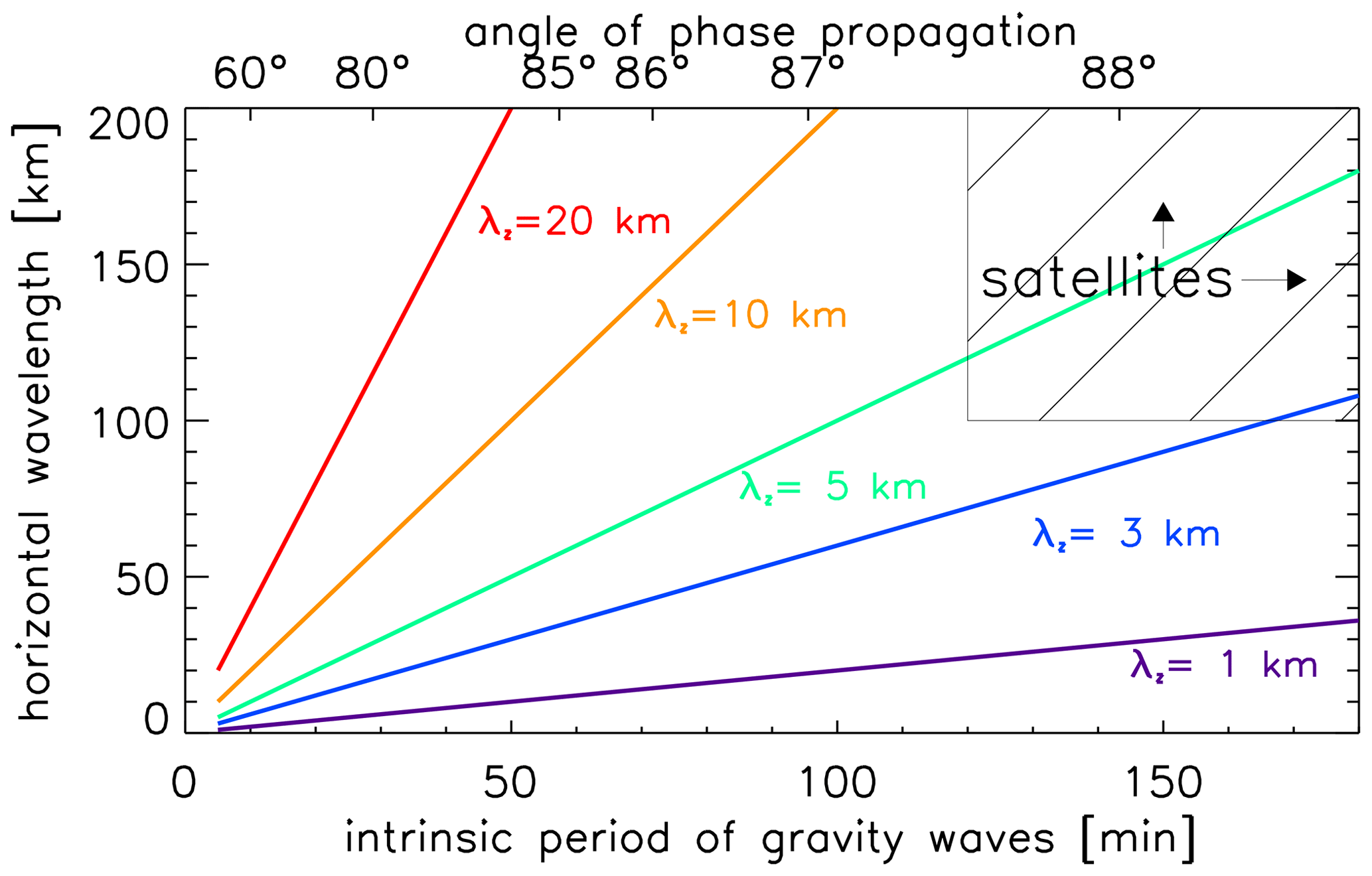
Figure 12Scales of gravity waves relevant for VAHCOLI deduced from the dispersion relation of gravity waves for mid-frequencies (Eq. 9). Horizontal wavelengths are shown as a function of intrinsic period for various vertical wavelengths (colored lines). The angle of phase propagation relative to the horizontal direction is given on the top abscissa. The hatched area (top right) indicates the lower part of ranges covered by satellites.
The aim of VAHCOLI is to characterize the three-dimensional time-dependent morphology of gravity waves. The comprehensive characterization of gravity wave propagation requires measuring the three-dimensional vector of phase propagation, i.e., the vertical and the horizontal components. Horizontal fluxes of gravity wave momentum are typically ignored (compared to vertical) in middle atmospheric modeling as it is often assumed that the effect of gravity waves takes place directly above the source and instantaneously. However, it is known from model studies that GWs can propagate over large horizontal distances before depositing momentum and energy (Alexander, 1996; Ehard et al., 2017; Stephan et al., 2020). Furthermore, a background varying with time can change the propagation of GWs (e.g., by refraction) and drastically modify the deposition of momentum and its effect on the background flow (Senf and Achatz, 2011). Simulations of GW propagation show that the horizontal distance between wave packets usually increases with altitude (see, for example, Alexander and Barnet, 2007). This is favorable for VAHCOLI since the horizontal distance between obliquely pointing beams also increases with altitude (see Fig. 11). Furthermore, it is known that the spatial and temporal distribution of gravity wave sources influences their effect on middle atmosphere dynamics (Šácha et al., 2016). A more fundamental question addresses the role of nonlinear interactions of gravity waves compared to a quasi-linear superposition. This leads to rather different concepts regarding gravity wave parametrization (Lindzen, 1981; Gavrilov, 1990; Fritts and Lu, 1993; Medvedev and Klaassen, 1995; Hines, 1997; Becker and Schmitz, 2002). It could well be that the applicability of one concept or the other depends on the temporal and spatial scales under consideration. In order to measure and study the effects outlined above it is obviously necessary to observe gravity waves in all directions over a longer period of several hours or even days and with sufficient horizontal coverage. Such instrumental capabilities are envisaged for VAHCOLI.
5.3 Stratified turbulence (ST)
The concept of stratified turbulence (ST) has recently been developed to explain the energy cascading in stratified flows at mesoscales as an alternative to classical linear or nonlinear breakdown of gravity waves. This transfer is relevant for momentum and energy budgets, which affect the Lorenz cycle and thereby (regional) climate modeling. Lindborg (2006) has developed an energy cascade theory for these scales in a strongly stratified fluid, which involves horizontal and vertical length scales as well as kinetic and potential energy. The theory of ST has recently been applied to wind measurements by radars in the mesopause region (Chau et al., 2020).
ST resembles the well-known energy spectra (horizontal kinetic energy and potential energy) characterized by (Nastrom and Gage, 1985). This theory invokes strong nonlinearities (in contrast to 2D turbulence and to weakly nonlinear interacting gravity waves) and the cascading of energy from large to small scales (see, for example Billant and Chomaz, 2001; Lindborg, 2006; Brethouwer et al., 2007; Lindborg, 2007, and references therein). It covers horizontal scales smaller than synoptic scales (Lh) and larger than buoyancy (Lb) and Ozmidov (LO) scales, and it covers vertical scales between Lb and LO. The Ozmidov scale LO = describes the largest scales in classical isotropic Kolmogorov turbulence which are not effected by buoyancy (N∼ 0.02 s−1; ϵ is the energy dissipation rate of turbulence). The buoyancy scale Lb = (uh: typical horizontal velocities of ST) characterizes the largest vertical scale of stratified turbulence, whereas Lh = is the largest horizontal scale of ST structures. Variability at scales larger than Lh are related to large-scale processes dominated by the Coriolis force. Introducing typical Kolmogorov isotropic turbulence velocities, ut = , several relationships can be derived, such as and . The magnitude of the outer scale of ST (Lh) is typically a few hundred kilometers (see, for example Avsarkisov et al., 2021).
Table 2Length scales, typical velocities, time constants, and various ratios of length scales relevant for (stratified) turbulence. The scales are shown for two cases of Lh, namely Lh = 100 km and Lh=400 km, as well as for two cases of energy dissipation rates ϵ, namely ϵ=10 mW kg−1 and ϵ=100 mW kg−1. For the kinematic viscosity a value of ν=0.01 m2 s−1 was chosen, which is typical for an altitude of 45 km (note that ν increases exponentially with increasing height). See text for more details.

∗ ϵ (mW kg−1). All lengths are in meters, all velocities are in meters per second (m s−1), and all time constants are in minutes.
Order-of-magnitude estimates for velocities and time constants related to these scales are derived from expressions such as and . Applying typical values, namely N=0.02 s−1 (BV period: 5 min), ϵ=100 mW kg−1, and Lh = 100 km, results in the following order-of-magnitude values: Lb = 1.01 km, LO = 0.112 km, uh = 21 m s−1, ut = 2.24 m s−1, = 9.6, and τh = 77 min, respectively. A collection of relationships and representative values is presented in Table 2. A more detailed representation of spatial and temporal scales as well as velocities associated with stratified turbulence are shown in Fig. 13 for a large range of ϵ values. Note that most quantities depend on season, latitude, and altitude (regarding ϵ, see, for example, Lübken, 1997). Some dimensionless numbers are frequently used to characterize the relevance of physical processes. For example, the horizontal Froude number, which is the ratio of inertial to buoyancy forces, must be small to allow ST to exist: Frh≪1. Note that . Indeed, Frh is very small for the examples shown in Table 2. Another relevant parameter is the buoyancy Reynolds number, , which should be large for both ST and for the Kelvin–Helmholtz instability regime (ν: kinematic viscosity). In the height range from the lower stratosphere to the upper mesosphere, and considering turbulence intensities of ϵ=10 mW kg−1 and ϵ=100 mW kg−1, this parameter varies between Reb = 2.5 × 10⁵ and Reb = 25 and between Reb = 2.5 × 10⁶ and Reb = 250, respectively, i.e., Reb is indeed much larger than unity. We note that the requirements to cover ST scales, namely a vertical and horizontal resolution of 200 m and 2 km, respectively, a horizontal coverage of up to 200 km, and temporal and velocity resolutions of 10–20 min and 0.5–1 m s−1, respectively, are well within the instrumental capabilities of VAHCOLI. The temporal development of the flow is important to judge various forcings, energy injection, the conversion of Epot and Ekin, and the transition to stationary conditions (see, e.g., Lindborg, 2006).

Figure 13Typical scales relevant for stratified turbulence (ST) as a function of the turbulent energy dissipation rate (ϵ). Length scales (left axis): largest horizontal scales of ST (Lh, green), buoyancy scales (Lb, black), and Ozmidov scales (LO, blue). Typical timescales (τh, right red axis) and horizontal velocities (uh, right black axis) related to Lh are shown, as are typical turbulent velocities (ut). The red dotted line indicates a typical Brunt–Väisälä period (PB). All scales are shown for two cases, namely Lh=100 km (solid lines) and Lh=400 km (dashed lines). The scales are defined in Sect. 5.3. See also Table 2.
There are several aspects of ST theory which are particularly relevant for a comparison with observations which will be made by VAHCOLI. To address the question, if energy is cascading from large to small scales (“forward”) or the other way around (“inverse”) it is helpful to consider not only the horizontal kinetic energy spectra (typically from aircraft observations) but also the vertical spectra of horizontal kinetic and potential energy typically derived from balloon-borne observations (Li and Lindborg, 2018; Alisse and Sidi, 2000; Hertzog et al., 2002). Note that a fundamental scale invariance of the Boussinesq equations in the limit of strong stratification implies an equi-partitioning of potential and kinetic energy (Billant and Chomaz, 2001). Regarding spectra, the ST theory (invoking downscale energy flow) predicts that vorticity Φ(k) and divergence Ψ(k) spectra should be of similar magnitude, Φ(k)≈Ψ(k), whereas for spectra dominated by gravity waves one would expect Φ(k)≪Ψ(k), and for stratified turbulence dominated by vortical coherent structures one expects Φ(k)≫Ψ(k). Furthermore, it is helpful to measure spectra of longitudinal and transversal velocity structure functions simultaneously (Lindborg, 2007).
In summary, the expected horizontal and vertical coverage of the flow field by VAHCOLI will allow us to study details of the relationship between rotational and divergent components of mesoscale dynamics including the important question of how energy is transferred from large to small scales. The instrumental capabilities of VAHCOLI will cover spatial and temporal scales which are highly relevant for mesoscale studies. Apart from the Helmholtz decomposition there are other important quantities, such as helicity, , which may be helpful to separate vortical coherent structures from GWs and to characterize the flow and its potential impact on the background atmosphere (Marino et al., 2013). Again, such a comprehensive analysis requires a 3D characterization of the flow field, as is envisaged for VAHCOLI.
5.4 Other dynamical parameters
There are several dynamical processes in the atmosphere which take place at spatial or temporal scales normally outside the range of VAHCOLI, at least for the time being. For example, the smallest scales of inertial range turbulence are on the order of . Measuring fluctuations at Lη scales offers a unique chance to unambiguously determine ϵ (Lübken, 1992). However, Lη varies by several orders of magnitude from the troposphere to the upper mesosphere ranging from centimeters to several meters only. It will be challenging to detect fluctuations at these small scales by, for example, placing several VAHCOLI units very close to each other. On the other hand, measuring the longitudinal and transversal structure functions of winds and temperatures at somewhat larger scales also allows us to derive reasonable estimates of ϵ. Furthermore, we envisage measuring the spectral broadening of the stratospheric aerosol signal to an extent that will allow us to deduce turbulent velocities. Note that typical turbulent velocities are on the order of 1 m s−1 (see Table 2), which corresponds to a spectral broadening of the Mie peak of 2.5 MHz. This is much larger than the Doppler broadening of the Mie peak due to Brownian motions (roughly 0.1 MHz).
Trace constituents may sometimes be used as passive tracers for transport and mixing. This mainly concerns vertical and horizontal advection and mixing of stratospheric aerosols and noctilucent clouds, but also the transport of metal atoms. Care needs to be taken when interpreting such measurements since these constituents may not be passive tracers; i.e., they may experience modifications, for example, by variable background temperatures. In the future we envisage measuring small-scale turbulence (see above) and improving the spatial resolution of aerosol observations to such an extent that the eddy correlation technique for measuring turbulent transport could be applicable.
On the other side of the spectrum of scales, tides are global-scale phenomena with horizontal wavelengths of several hundred kilometers. Certainly, the relevant periods and vertical wavelengths are within the scope of standard lidars (see Baumgarten et al., 2018, for a recent example). Regarding horizontal wavelengths, one could consider placing several VAHCOLI units at very large distances.
Dynamical phenomena are frequently characterized by calculating statistical quantities, such as the variance and higher moments (skewness, kurtosis, etc.) as well as intermittency. Due to the operational advantages of VAHCOLI (low cost, unattended operation, low infrastructure demands, long-term stability, etc.) there is an opportunity to extend such an analysis to bivariate or multivariate distributions, for example, by correlating wind components at various places with each other or with temperatures.
5.5 NLCs, PSCs, background aerosols, and metal densities
Layers of ice particles in the summer mesosphere at middle and polar latitudes are known as NLCs (“noctilucent clouds”) (Gadsden and Schröder, 1989). They exhibit a large range of temporal and spatial variability which can be observed even by the naked eye or by cameras. Most of these variations are presumably related to gravity waves, tides, and associated instability processes (see Baumgarten and Fritts, 2014, for a more recent example). NLCs are studied in great detail by modern, lidars which sometimes detect temporal fluctuations on timescales down to seconds or other unexpected characteristics (Hansen et al., 1989; Alpers et al., 2001; Gardner et al., 2001; Kaifler et al., 2013). NLCs are frequently used in models describing dynamical phenomena such as gravity wave breaking (Fritts et al., 2017). This raises the following question: up to what scales can NLCs be treated as passive tracers? Note that several processes act on similar temporal and spatial scales: for example, nucleation, sedimentation, and horizontal transport. Furthermore, there is an impressive number of observations of mesospheric ice clouds available from satellites, which sometimes show unexpected temporal and/or spatial variations (“voids”) (see Russell et al., 2009, for more details on a recent satellite mission dedicated to NLC science). Understanding the physics of NLCs is important, for example, to interpret long-term variations of layers of ice particles and their potential relation to climate change (Thomas, 1996; von Zahn, 2003; Lübken et al., 2018). Similar science questions occur regarding PSCs, which, amongst others, play a crucial role in ozone chemistry. Very thin layers of background aerosols have been observed in the stratosphere, which are presumably caused by intrusion of midlatitude air into the winter polar vortex (see, for example, Plumb et al., 1994; Langenbach et al., 2019). Several VAHCOLI units could be placed at appropriate locations, e.g., at the edge of the polar vortex, to observe the temporal and spatial development of such intrusions.
For solving some of the open science questions regarding NLCs, PSCs, and background aerosols, it is very helpful to distinguish between temporal and spatial (horizontal) variations and to know the status of the background atmosphere. VAHCOLI is designed to detect these aerosol fluctuations and to observe background temperatures and winds simultaneously by applying high-resolution spectral filtering (see Sect. 2.5.2).
Despite substantial progress in recent years, the physics and chemistry of metal layers still leave many open questions, for example, regarding their (meteoric) origin, their spatial and seasonal distribution, the impact of diffusion and turbulent transport, and the effect of gravity waves and tides on number density profiles (see Plane, 2003, for a recent review on mesospheric metals). The morphology of metal profiles offers a variety of phenomena on short spatial and temporal scales, such as sudden (sporadic) layers and their connection to ionospheric processes, as well as the uptake of metal densities on ice particles (see, e.g., Hansen and von Zahn, 1990; Alpers et al., 1993; Collins et al., 1996; Plane et al., 2004; Lübken and Höffner, 2004). Many of these anomalies can best be studied by distinguishing temporal from spatial variations. VAHCOLI is designed to observe metal layers (potassium for now) at various locations with high time resolution.
Several improvements regarding the technical performance of lidars being used for VAHCOLI are currently in progress or are foreseen for the near future. This concerns, for example, the optical layout of the telescope, the development of multi-beam operation, and the output of the power laser. A power increase of up to several Watts by applying ring-laser technology is currently under development, even without employing a separate amplification stage. The VAHCOLI units are designed to be extended to further wavelengths, for example, by installing a second seeder laser and an SHG (second harmonic generation) to simultaneously apply resonance scattering on potassium (λ = 770 nm) and iron (λ = 386 nm) during both night and day. Stimulated Raman emission may also be considered for producing laser light in the infrared.
The robust and compact design of the VAHCOLI units and their stand-alone operation capability allow us to consider somewhat extraordinary operations, for example, on airplanes, balloons, ships, or trains and at remote places such as Spitsbergen or Antarctica. Some of these applications have been proven to be realistic but so far with substantial effort regarding technical realization, man power, and costs (von Zahn et al., 1996; Höffner and Lübken, 2007; Lübken et al., 2017; Chu et al., 2018). VAHCOLI may also be extended to other wavelengths relevant for thermospheric or space applications (Höffner et al., 2018; Munk et al., 2018; Höffner et al., 2019). Due to its compact design and autonomous operation a VAHCOLI unit may also be of interest for measurements from satellites (Strotkamp et al., 2019). The final aim is to further improve the VAHCOLI units and to develop a cost-effective multi-purpose lidar with several systems that may be employed at various locations and be operated quasi-autonomously.
In summary, we have presented the VAHCOLI concept, which consists of a cluster of lidars (units) to study the middle atmosphere in four dimensions, namely high temporal, vertical, and horizontal resolution and coverage. The concept relies on the development of a new type of lidar which is compact (∼ 1 m3), can be operated stand-alone during night and day (even under harsh field conditions), and still offers a performance which is comparable to, or even better compared to, existing lidars. The innovative approach for this lidar is based on very fast and high-spectral-resolution spectroscopy. Apart from a narrowband spectral filter in the detector system (confocal etalon: 7.5 MHz) the key component of the new lidar is a newly developed diode-pumped alexandrite laser offering a small line width of ∼ 3.3 MHz, which is significantly better compared to most lasers currently being used in lidars (e.g., Nd:YAG and lasers pumped by Nd:YAG: ∼ 50–100 MHz). The laser is flexible and can be tuned quickly over, for example, a Doppler-broadened line originating from atmospheric Rayleigh or resonance scattering. At the same time, the laser can also cover a large frequency range and may be used for other absorption lines. The flexibility of the lidar allows us to optimize system performance at certain height ranges or concentrate on the measurement of specific atmospheric parameters: for example, measuring winds from stratospheric aerosols or temperatures from resonance scattering in the upper mesosphere–lower thermosphere. For the first time, temperatures and winds from Rayleigh and/or resonance scattering can be deduced in the presence of aerosols (stratospheric aerosols, noctilucent clouds). The compact layout of the lidar reduces the difficulties associated with optical alignment. Since these lidars allow for autonomous operation under harsh field conditions at remote locations, they are ideally suited for the VAHCOLI concept, namely to employ a cluster of these units to simultaneously cover atmospheric parameters in the vertical and horizontal direction with sufficient spatial and temporal resolution. The units will be cost-effective using off-the-shelf components and 3D-printed mechanical subsystems. In this paper we have discussed some relevant science applications of such observations, for example, regarding gravity waves and stratified turbulence. We have presented measurements from a first prototype of such a lidar demonstrating the suitability of the new lidar for VAHCOLI. This paper has addressed just a selection of the numerous future application scenarios of VAHCOLI.
Data are available at https://doi.org/10.22000/405 (Lübken, 2020).
JH designed the lidar and provided some of the data shown in the paper; FJL prepared the paper (with contributions from JH) and some of the plots.
The authors declare that they have no conflict of interest.
The contribution, support, and expertise of the Fraunhofer Institute for Laser Technology (ILT) in Aachen when developing a new laser are highly appreciated. Alsu Mauer, Jan Froh, and Thorben Mense have contributed substantially to the technical development of the lidar being used in VAHCOLI. We thank Victor Avsarkisov, Gerd Baungarten, Erich Becker, Koki Chau, and Michael Gerding for helpful discussions and Gerd Baumgarten for providing the ECMWF data. We appreciate the comments from Robin Wing on some language issues.
This research has been supported by the Leibniz SAW project FORMOSA (grant no. K227/2019), the DFG project PACOG (grant no. LU-1174/8-1), which is part of the MSGWaves research group, and by the BMWi project ALISE (grant no. FKZ 50RP1605).
This paper was edited by Gabriele Stiller and reviewed by three anonymous referees.
Alexander, M. J.: A simulated spectrum of convectively generated gravity waves: propagation from the tropopause to the mesopause and effects in the middle atmosphere, J. Geophys. Res., 101, 1571–1588, 1996. a
Alexander, M. J. and Barnet, C.: Using satellite observations to constrain parameterizations of gravity wave effects for global models, J. Atmos. Sci., 64, 1652–1665, https://doi.org/10.1175/JAS3897.1, 2007. a
Alexander, M. J., Geller, M., McLandress, C., Polavarapu, S., Preusse, P., Sassi, F., Sato, K., Eckermann, S., Ern, M., Hertzog, A., Kawatani, Y., Pulido, M., Shaw, T., Sigmond, M., Vincent, R., and Watanabe, S.: A review of recent developments on gravity wave effects in climate models and the global distribution of gravity wave momentum flux, Q. J. Roy. Meteor. Soc., 136, 1103–1124, https://doi.org/10.1002/qj.637, 2010. a
Alisse, J.-R. and Sidi, C.: Experimental probability density functions of small-scale fluctuations in the stably stratified atmosphere, J. Fluid Mech., 402, 137–162, 2000. a
Alpers, M., Höffner, J., and von Zahn, U.: Iron atom densities in the polar mesossphere from lidar observations, Geophys. Res. Lett., 17, 2345–2348, 1990. a
Alpers, M., Höffner, J., and von Zahn, U.: Sporadic Fe and E-layers at polar, middle, and low latitudes, J. Geophys. Res., 98, 275–283, 1993. a
Alpers, M., Gerding, M., Höffner, J., and von Zahn, U.: NLC particle properties from a five-color observation at 54∘ N, J. Geophys. Res., 105, 12235–12240, 2000. a
Alpers, M., Gerding, M., Höffner, J., and Schneider, J.: Multiwavelength lidar observation of a strange noctilucent cloud at Kühlungsborn, Germany (54∘ N), J. Geophys. Res., 106, 7945–7953, 2001. a
Avsarkisov, V., Becker, E., and Renkwitz, T.: Turbulent parameters in the middle atmosphere: theoretical estimates deduced from a gravity-wave resolving general circulation model, J. Atmos. Sci., submitted, 2021. a
Baumgarten, G.: Doppler Rayleigh/Mie/Raman lidar for wind and temperature measurements in the middle atmosphere up to 80 km, Atmos. Meas. Tech., 3, 1509–1518, https://doi.org/10.5194/amt-3-1509-2010, 2010. a
Baumgarten, G. and Fritts, D. C.: Quantifying Kelvin-Helmholtz instability dynamics observed in noctilucent clouds: 1. methods and observations, J. Geophys. Res.-Atmos., 119, 9324–9337, https://doi.org/10.1002/2014JD021832, 2014. a
Baumgarten, G., Fiedler, J., and Rapp, M.: On microphysical processes of noctilucent clouds (NLC): observations and modeling of mean and width of the particle size-distribution, Atmos. Chem. Phys., 10, 6661–6668, https://doi.org/10.5194/acp-10-6661-2010, 2010. a
Baumgarten, G., Fiedler, J., Hildebrand, J., and Lübken, F.-J.: Inertia gravity wave in the stratosphere and mesosphere observed by Doppler wind and temperature lidar, Geophys. Res. Lett., 42, 10929–10936, https://doi.org/10.1002/2015GL066991, 2015. a, b
Baumgarten, K., Gerding, M., and Lübken, F.-J.: Seasonal variation of gravity wave parameters using different filter methods with daylight lidar measurements at mid-latitudes, J. Geophys. Res.-Atmos., 122, 2683–2695, https://doi.org/10.1002/2016JD025916, 2017. a
Baumgarten, K., Gerding, M., Baumgarten, G., and Lübken, F.-J.: Temporal variability of tidal and gravity waves during a record long 10-day continuous lidar sounding, Atmos. Chem. Phys., 18, 371–384, https://doi.org/10.5194/acp-18-371-2018, 2018. a
Becker, E.: Frictional heating in global climate models, Mon. Weather Rev., 131, 508–520, 2003. a
Becker, E. and Schmitz, G.: Energy deposition and turbulent dissipation owing to gravity waves in the mesosphere, J. Atmos. Sci., 59, 54–68, 2002. a
Becker, E. and Vadas, S. L.: Secondary gravity waves in the winter mesosphere: results from a high-resolution global circulation model, J. Geophys. Res.-Atmos., 123, 2605–2627, https://doi.org/10.1002/2017JD027460, 2018. a
Billant, P. and Chomaz, J.-M.: Self-similarity of strongly stratified inviscid flows, Phys. Fluids, 13, 1645–1651, https://doi.org/10.1063/1.1369125, 2001. a, b
Brethouwer, G., Billant, P., Lindborg, E., and Chomaz, J.-M.: Scaling analysis and simulation of strongly stratified turbulent flows, J. Fluid Mech., 585, 343–368, https://doi.org/10.1017/S0022112007006854, 2007. a
Chanin, M. L., Garnier, A., Hauchecorne, A., and Porteneuve, J.: A Doppler lidar for measuring winds in the middle atmosphere, Geophys. Res. Lett., 16, 1273–1276, https://doi.org/10.1029/GL016i011p01273, 1989. a
Chau, J. L., Stober, G., Hall, C. M., Tsutsumi, M., Laskar, F. I., and Hoffmann, P.: Polar mesospheric horizontal divergence and relative vorticity measurements using multiple specular meteor radars, Radio Sci., 52, 811–828, https://doi.org/10.1002/2016RS006225, 2017. a
Chau, J. L., Urco, J. M., Avsarkisov, V., Vierinen, J. P., Latteck, R., Hall, C. M., and Tsutsumi, M.: Four-dimensional quantification of Kelvin-Helmholtz instabilities in the polar summer mesosphere using volumetric radar imaging, Geophys. Res. Lett., 47, e2019GL086081, https://doi.org/10.1029/2019GL086081, 2020. a
Chu, X., Gardner, C. S., and Franke, S. J.: Nocturnal thermal structure of the mesosphere and lower thermosphere region at Maui, Hawaii (20.7∘ N), and Starfire Optical Range, New Mexico (35∘ N), J. Geophys. Res.-Atmos., 110, D09S03, https://doi.org/10.1029/2004JD004891, 2005. a
Chu, X., Yu, Z., Gardner, C. S., Chen, C., and Fong, W.: Lidar observations of neutral Fe layers and fast gravity waves in the thermosphere (110–155 km) at McMurdo (77.8∘ S, 166.7∘ E), Antarctica, Geophys. Res. Lett., 38, L23807, https://doi.org/10.1029/2011GL050016, 2011. a, b
Chu, X., Zhao, J., Lu, X., Harvey, V. L., Jones, R. M., Becker, E., Chen, C., Fong, W., Yu, Z., Roberts, B. R., and Dörnbrack, A.: Lidar observations of stratospheric gravity waves from 2011 to 2015 at McMurdo 77.84∘ S, 166.69∘ E, Antarctica: 2. potential energy densities, lognormal distributions and seasonal variation, J. Geophys. Res.-Atmos., 123, 7910–7934, https://doi.org/10.1029/2017JD027386, 2018. a, b
Clemesha, B. R.: Sporadic neutral metal layers in the mesosphere and lower thermosphere, J. Atmos. Terr. Phys., 57, 725–736, 1995. a
Collins, R. L., Hallinan, T. J., Smith, R. W., and Hernandez, G.: Lidar observations of a large high-altitude sporadic Na layer during active aurora, Geophys. Res. Lett., 23, 3655–3658, 1996. a
Collins, R. L., Taylor, M. J., Nielsen, K., Mizutani, K., Murayama, Y., Sakanoi, K., and DeLand, M. T.: Noctilucent cloud in the western Arctic in 2005: simultaneous lidar and camera observations and analysis, J. Atmos. Sol.-Terr. Phy., 71, 446–452, https://doi.org/10.1016/j.jastp.2008.09.044, 2009. a
Dörnbrack, A., Gisinger, S., and Kaifler, B.: On the interpretation of gravity wave measurements by ground-based lidars, Atmosphere, 8, 48, https://doi.org/10.3390/atmos8030049, 2017. a
Ehard, B., Kaifler, B., Dörnbrack, A., Preusse, P., Eckermann, S. D., Bramberger, M., Gisinger, S., Kaifler, N., Liley, B., Wagner, J., Rapp, M., and Mahlman, J. D.: Horizontal propagation of large-amplitude mountain waves into the polar night jet, J. Geophys. Res.-Atmos., 122, 1423–1436, https://doi.org/10.1002/2016JD025621, 2017. a
Ern, M., Preusse, P., Alexander, M. J., and Warner, C. D.: Absolute values of gravity wave momentum flux derived from satellite data, J. Geophys. Res.-Atmos., 109, D20103, https://doi.org/10.1029/2004JD004752, 2004. a
Fiedler, J., Baumgarten, G., and Lübken, F.-J.: NLC observations during one solar cycle above ALOMAR, J. Atmos. Sol.-Terr. Phy., 71, 424–433, https://doi.org/10.1016/j.jastp.2008.11.010, 2009. a
Fricke, K. and von Zahn, U.: Mesopause temperatures derived from probing the hyperfine structure of the D2 resonance line of sodium by lidar, J. Atmos. Terr. Phys., 47, 499–512, 1985. a
Fritts, D. C. and Alexander, J.: Gravity wave dynamics and effects in the middle atmosphere, Rev. Geophys., 41, 1003, https://doi.org/10.1029/2001RG000106, 2003. a, b
Fritts, D. C. and Lu, W.: Spectral estimates of gravity wave energy and momentum fluxes, II: parameterization of wave forcing and variability, J. Atmos. Sci., 50, 3695–3713, 1993. a
Fritts, D. C., Wang, L., Baumgarten, G., Miller, A. D., Geller, M. A., Jones, G., Limon, M., Chapman, D., Didier, J., Kjellstrand, C. B., Araujo, D., Hillbrand, S., Korotkov, A., Tucker, G., and Vinokurov, J.: High resolution observations and modeling of turbulence sources, structures, and intensities in the upper mesosphere, J. Atmos. Sol.-Terr. Phy., 162, 57–78, https://doi.org/10.1016/j.jastp.2016.11.006, 2017. a
Fritts, D. C., Kaifler, N., Kaifler, B., Geach, C., Kjellstrand, C. B., Williams, B. P., Eckermann, S. D., Miller, A. D., Rapp, M., Jones, G., Limon, M., Reimuller, J., and Wang, L.: Mesospheric bore evolution and instability dynamics observed in PMC TURBO imaging and Rayleigh lidar profiling over North-Eastern Canada on 13 July 2018, J. Geophys. Res.-Atmos., 125, e2019JD032037, https://doi.org/10.1029/2019JD032037, 2020. a
Gadsden, M. and Schröder, W.: Noctilucent clouds, Springer-Verlag, New York, USA, 1989. a
Gardner, C. S., Papen, G. C., Chu, X., and Pan, W.: First lidar observations of middle atmosphere temperatures, Fe densities, and polar mesospheric clouds over the North and South Poles, Geophys. Res. Lett., 28, 1199–1202, 2001. a, b
Gavrilov, N. M.: Parameterization of accelerations and heat flux divergences produced by internal gravity waves in the middle atmosphere, J. Atmos. Terr. Phys., 52, 707–713, 1990. a
Gerding, M., Alpers, M., von Zahn, U., Rollason, R. J., and Plane, J. M. C.: Atmospheric Ca and Ca+ layers: mid-latitude observations and modeling, J. Geophys. Res., 105, 27131–27146, 2000. a
Hansen, G. and von Zahn, U.: Sudden sodium layers in polar latitudes, J. Atmos. Terr. Phys., 52, 585–608, 1990. a
Hansen, G., Serwazi, M., and von Zahn, U.: First detection of a noctilucent cloud by lidar, Geophys. Res. Lett., 16, 1445–1448, 1989. a
Hauchecorne, A. and Chanin, M.: Density and temperature profiles obtained by lidar between 35 and 70 km, Geophys. Res. Lett., 7, 565–568, 1980. a, b
Hertzog, A., Vial, F., Mechoso, C. R., Basdevant, C., Cocquerez, P., Dubourg, V., and Nouel, F.: Planetary and gravity wave activity in the equatorial lower stratosphere as seen by ultra-long duration balloons, Adv. Space Res., 30, 1381–1386, https://doi.org/10.1016/S0273-1177(02)00555-0, 2002. a
Hines, C. O.: Doppler-spread parameterization of gravity-wave momentum deposition in the middle atmosphere: part 1: basic formulation, J. Atmos. Terr. Phys., 59, 371–386, 1997. a
Höffner, J. and Lautenbach, J.: Daylight measurements of mesopause temperature and vertical wind with the mobile scanning iron lidar, Opt. Lett., 34, 1351–1353, 2009. a
Höffner, J. and Lübken, F.-J.: Potassium lidar temperatures and densities in the mesopause region at Spitsbergen (78∘ N), J. Geophys. Res.-Atmos., 112, D20114, https://doi.org/10.1029/2007JD008612, 2007. a, b, c
Höffner, J. and von Zahn, U.: Mesopause temperature profiling by potassium lidar: recent progress and outlook for ALOMAR, in: Proceedings of the 12th ESA Symposium on European Rocket and Balloon Programmes and Related Research (ESA SP-370), 29 May 1995, Lillehammer, Norway, edited by: Kaldeich-Schürmann, B., 403–407, 1995. a
Höffner, J., Strotkamp, M., Munk, A., and Jungbluth, B.: Demonstration of a compact and universal Doppler lidar based on a novel diode pumped alexandrite ring laser, in: Proc. SPIE 11180, International Conference on Space Optics – ICSO 2018, Chania, Greece, 9–12 October 2018, 1118029, https://doi.org/10.1117/12.2536000, 2018. a, b
Höffner, J., Froh, J., Mauer, A., Lübken, F., Strotkamp, M., Munk, A., and Jungblut, B.: A novel diode pumped alexandrite ring laser for Doppler lidar, in: 2019 Conference on Lasers and Electro-Optics Europe European Quantum Electronics Conference (CLEO/Europe-EQEC), 23 June 2019, Munich, Germany, 19148241, 2019. a
Kaifler, B. and Kaifler, N.: A Compact Rayleigh Autonomous Lidar (CORAL) for the middle atmosphere, Atmos. Meas. Tech., 14, 1715–1732, https://doi.org/10.5194/amt-14-1715-2021, 2021. a
Kaifler, B., Lübken, F.-J., Höffner, J., Morris, R. J., and Viehl, T. P.: Lidar observations of gravity wave activity in the middle atmosphere over Davis (69∘ S, 78∘ E), Antarctica, J. Geophys. Res.-Atmos., 120, 4506–4521, https://doi.org/10.1002/2014JD022879, 2015. a
Kaifler, N., Baumgarten, G., Fiedler, J., and Lübken, F.-J.: Quantification of waves in lidar observations of noctilucent clouds at scales from seconds to minutes, Atmos. Chem. Phys., 13, 11757–11768, https://doi.org/10.5194/acp-13-11757-2013, 2013. a
Kaifler, N., Kaifler, B., Ehard, B., Gisinger, S., Dörnbrack, A., Rapp, M., Kivi, R., Kozlovsky, A., Lester, M., and Liley, B.: Observational indications of downward-propagating gravity waves in middle atmosphere lidar data, J. Atmos. Sol.-Terr. Phy., 162, 16–27, https://doi.org/10.1016/j.jastp.2017.03.003, 2017. a
Keckhut, P., Hauchecorne, A., and Chanin, M.-L.: Midlatitude long-term variability of the middle atmosphere, J. Geophys. Res., 100, 18887–18897, 1995. a
Langenbach, A., Baumgarten, G., Fiedler, J., Lübken, F.-J., von Savigny, C., and Zalach, J.: Year-round stratospheric aerosol backscatter ratios calculated from lidar measurements above northern Norway, Atmos. Meas. Tech., 12, 4065–4076, https://doi.org/10.5194/amt-12-4065-2019, 2019. a, b
Li, Q. and Lindborg, E.: Weakly or strongly nonlinear mesoscale dynamics close to the tropopause?, J. Atmos. Sci., 75, 1215–1229, https://doi.org/10.1175/JAS-D-17-0063.1, 2018. a
Lindborg, E.: The energy cascade in a strongly stratified fluid, J. Fluid Mech., 550, 207–242, https://doi.org/10.1017/S0022112005008128, 2006. a, b, c
Lindborg, E.: Horizontal wavenumber spectra of vertical vorticity and horizontal divergence in the upper troposphere and lower stratosphere, J. Atmos. Sci., 64, 1017–1025, https://doi.org/10.1175/JAS3864.1, 2007. a, b
Lindzen, R. S.: Turbulence and stress owing to gravity wave and tidal breakdown, J. Geophys. Res., 86, 9707–9714, 1981. a
Liu, A. Z. and Gardner, C. S.: Vertical heat and constituent transport in the mesopause region by dissipating gravity waves at Maui, Hawaii (20.7∘ N), and Starfire Optical Range, New Mexico (35∘ N), J. Geophys. Res.-Atmos., 110, D09S13, https://doi.org/10.1029/2004JD004965, 2005. a
Lübken, F.-J.: On the extraction of turbulent parameters from atmospheric density fluctuations, J. Geophys. Res., 97, 20385–20395, 1992. a
Lübken, F.-J.: Seasonal variation of turbulent energy dissipation rates at high latitudes as determined by insitu measurements of neutral density fluctuations, J. Geophys. Res., 102, 13441–13456, 1997. a
Lübken, F.-J. and Höffner, J.: Experimental evidence for ice particle interaction with metal atoms at the high latitude summer mesopause region, Geophys. Res. Lett., 31, L08103, https://doi.org/10.1029/2004GL019586, 2004. a
Lübken, F.-J.: Luebken-AMT-2021, Leibniz-Institute of Atmospheric Physics [data set], https://doi.org/10.22000/405, 2020. a
Lübken, F.-J., Zecha, M., Höffner, J., and Röttger, J.: Temperatures, polar mesosphere summer echoes, and noctilucent clouds over Spitsbergen (78∘ N), J. Geophys. Res.-Atmos., 109, D11203, https://doi.org/10.1029/2003JD004247, 2004. a
Lübken, F.-J., Latteck, R., Becker, E., Höffner, J., and Murphy, D.: Using polar mesosphere summer echoes and stratospheric/mesospheric winds to explain summer mesopause jumps in Antarctica, J. Atmos. Sol.-Terr. Phy., 162, 106–115, https://doi.org/10.1016/j.jastp.2016.06.008, 2017. a
Lübken, F.-J., Berger, U., and Baumgarten, G.: On the anthropogenic impact on long-term evolution of noctilucent clouds, Geophys. Res. Lett., 45, 6681–6689, https://doi.org/10.1029/2018GL077719, 2018. a
Marino, R., Mininni, P. D., Rosenberg, D., and Pouquet, A.: On the emergence of helicity in rotating stratified turbulence, Phys. Rev. E, 87, 3, https://doi.org/10.1103/PhysRevE.87.033016, 2013. a
Medvedev, A. S. and Klaassen, G. P.: Vertical evolution of gravity wave spectrs and the parameterization of associated wave drag, J. Geophys. Res., 100, 25841–25853, 1995. a
Munk, A., Jungbluth, B., Strothkamp, M., Hoffmann, H.-D., Poprawe, R., Höffner, J., and Lübken, F.-J.: Diode-pumped alexandrite ring laser in single-longitudinal mode operation for atmospheric lidar measurements, Opt. Express, 26, 1428–1435, https://doi.org/10.1364/OE.26.014928, 2018. a
Nastrom, G. D. and Gage, K. S.: A climatology of atmospheric wavenumber spectra of wind and temperature observed by commercial aircraft, J. Atmos. Sci., 42, 950–960, 1985. a, b
Nicklaus, K., Morasch, V., Hoefer, M., Luttmann, J., Vierkoetter, M., Ostermeyer, M., Höffner, J., Lemmerz, C., and Hoffmann, D.: Frequency stabilization of Q-switched Nd:YAG oscillators for airborne and spaceborne lidar systems, in: Proceedings of SPIE 6451 – Solid State Lasers XVI: Technology and Devices, Lasers and Applications in Science and Engineering, San Jose, California, USA, 20–25 January 2007, 645101, https://doi.org/10.1117/12.701187, 2007. a
Pautet, P. D., Taylor, M. J., Pendleton, W. R., Zhao, Y., Yuan, T., Esplin, R., and McLain, D.: Advanced mesospheric temperature mapper for high-latitude airglow studies, Appl. Optics, 53, 5934–5943, https://doi.org/10.1364/AO.53.005934, 2015. a, b
Plane, J.: Atmospheric chemistry of meteoric metals, Chem. Rev., 103, 4963–4984, 2003. a
Plane, J., Murray, B., Chu, X., and Gardner, C.: Removal of meteoric iron on polar mesosphere clouds, Science, 304, 426–428, 2004. a
Plumb, R. A., Waugh, D. W., Atkinson, R. J., Newman, P. A., Lait, L. R., Schoeberl, M. R., Browell, E. V., Simmons, A. J., and Loewenstein, M.: Intrusions into the lower stratospheric Arctic vortex during the winter of 1991–1992, J. Geophys. Res.-Atmos., 99, 1089–1105, https://doi.org/10.1029/93JD02557, 1994. a
Preusse, P., Eckermann, S. D., and Ern, M.: Transparency of the atmosphere to short horizontal wavelength gravity waves, J. Geophys. Res.-Atmos., 113, D24104, https://doi.org/10.1029/2007JD009682, 2008. a
Rauthe, M., Gerding, M., and Lübken, F.-J.: Seasonal changes in gravity wave activity measured by lidars at mid-latitudes, Atmos. Chem. Phys., 8, 6775–6787, https://doi.org/10.5194/acp-8-6775-2008, 2008. a
Reitebuch, O.: The spaceborne wind lidar mission ADM-Aeolus, Springer Berlin, Heidelberg, Germany, 815–827, https://doi.org/10.1007/978-3-642-30183-4_49, 2012. a
Rüfenacht, R., Baumgarten, G., Hildebrand, J., Schranz, F., Matthias, V., Stober, G., Lübken, F.-J., and Kämpfer, N.: Intercomparison of middle-atmospheric wind in observations and models, Atmos. Meas. Tech., 11, 1971–1987, https://doi.org/10.5194/amt-11-1971-2018, 2018. a
Russell III, J. M., Bailey, S. M., Gordley, L. L., Rusch, D. W., Horányi, M., Hervig, M. E., Thomas, G. E., Randall, C. E., Siskind, E. D., Stevens, M. H., Summers, M. E., Taylor, M. J., Englert, C. R., Espy, P. J., McClintock, W. E., and Merkel, A. W.: The Aeronomy of Ice in the Mesosphere (AIM) mission: overview and early science results, J. Atmos. Sol.-Terr. Phy., 71, 289–299, https://doi.org/10.1016/j.jastp.2008.08.011, 2009. a
Šácha, P., Lilienthal, F., Jacobi, C., and Pišoft, P.: Influence of the spatial distribution of gravity wave activity on the middle atmospheric dynamics, Atmos. Chem. Phys., 16, 15755–15775, https://doi.org/10.5194/acp-16-15755-2016, 2016. a
Senf, F. and Achatz, U.: On the impact of middle-atmosphere thermal tides on the propagation and dissipation of gravity waves, J. Geophys. Res.-Atmos., 116, D24110, https://doi.org/10.1029/2011JD015794, 2011. a
She, C. Y. and Yu, J. R.: Simultaneous three-frequency Na lidar measurements of radial wind and temperature in the mesopause region, Geophys. Res. Lett., 21, 1771–1774, https://doi.org/10.1029/94GL01417, 1994. a
She, C. Y., Latifi, H., Yu, J. R., Alvarez II, R. J., Bills, R. E., and Gardner, C. S.: Two-frequency lidar technique for mesospheric Na temperature measurements, Geophys. Res. Lett., 17, 929–932, 1990. a
She, C. Y., Yu, J. R., Krueger, D. A., Roble, R., Keckhut, P., Hauchecorne, A., and Chanin, M.-L.: Vertical structure of the mid-latitude temperature from stratosphere to mesopause (30–105 km), Geophys. Res. Lett., 22, 377–380, 1995. a
Shepherd, O., Aurilio, G., Hurd, A. G., Rappaport, S. A., Reidy, W. P., Rieder, R. J., Bedo, D. E., and Swirbalus, R. A.: Balloonborne lidar payloads for remote sensing, Adv. Space Res., 14, 95–100, 1994. a
Shepherd, T. G.: Atmospheric circulation as a source of uncertainty in climate change projections, Nat. Geosci., 7, 703–708, https://doi.org/10.1038/ngeo2253, 2014. a
Stephan, C. C., Schmidt, H., Zülicke, C., and Matthias, V.: Oblique gravity wave propagation during sudden stratospheric warmings, J. Geophys. Res.-Atmos., 125, e2019JD031528, https://doi.org/10.1029/2019JD031528, 2020. a
Strelnikova, I., Baumgarten, G., and Lübken, F.-J.: Advanced hodograph-based analysis technique to derive gravity-wave parameters from lidar observations, Atmos. Meas. Tech., 13, 479–499, https://doi.org/10.5194/amt-13-479-2020, 2020. a
Strelnikova, I., Almowafy, M., Baumgarten, G., Baumgarten, K., Ern, M., Gerding, M., and Lübken, F.-J.: Seasonal cycle of gravity wave potential energy density from lidar and satellite observations at 54∘ and 69∘ N, J. Atmos. Sci., 78, 1359–1386, https://doi.org/10.1175/JAS-D-20-0247.1, 2021. a
Strotkamp, M., Munk, A., Jungbluth, B., Hoffmann, H.-D., and Höffner, J.: Diode-pumped alexandrite laser for next generation satellite-based Earth observation lidar, CEAS Space Journal, 11, 413–422, https://doi.org/10.1007/s12567-019-00253-z, 2019. a, b
Thomas, G.: Is the polar mesosphere the miner's canary of global change?, Adv. Space Res., 18, 149–158, 1996. a
Vierinen, J., Chau, J. L., Charuvil, H., Urco, J. M., Clahsen, M., Avsarkisov, V., Marino, R., and Volz, R.: Observing mesospheric turbulence with specular meteor radars: a novel method for estimating second-order statistics of wind velocity, Earth Space Sci., 6, 1171–1195, https://doi.org/10.1029/2019EA000570, 2019. a
Voigt, C., Dörnbrack, A., Wirth, M., Groß, S. M., Pitts, M. C., Poole, L. R., Baumann, R., Ehard, B., Sinnhuber, B.-M., Woiwode, W., and Oelhaf, H.: Widespread polar stratospheric ice clouds in the 2015–2016 Arctic winter – implications for ice nucleation, Atmos. Chem. Phys., 18, 15623–15641, https://doi.org/10.5194/acp-18-15623-2018, 2018. a
von Cossart, G., Fiedler, J., and von Zahn, U.: Size distributions of NLC particles as determined from 3-color observations of NLC by ground-based lidar, Geophys. Res. Lett., 26, 1513–1516, 1999. a
von Zahn, U.: Are noctilucent clouds truly a “Miner's Canary” for global change?, EOS, 84, 261–264, 2003. a
von Zahn, U. and Höffner, J.: Mesopause temperature profiling by potassium lidar, Geophys. Res. Lett., 23, 141–144, 1996. a, b, c
von Zahn, U., Hansen, G., and Kurzawa, H.: Observations of the sodium layer at high latitudes in summer, Nature, 331, 594–596, https://doi.org/10.1038/331594a0, 1988. a, b, c
von Zahn, U., Höffner, J., Eska, V., and Alpers, M.: The mesopause altitude: only two distinctive levels worldwide?, Geophys. Res. Lett., 23, 3231–3234, 1996. a
von Zahn, U., von Cossart, G., Fiedler, J., Fricke, K. H., Nelke, G., Baumgarten, G., Rees, D., Hauchecorne, A., and Adolfsen, K.: The ALOMAR Rayleigh/Mie/Raman lidar: objectives, configuration, and performance, Ann. Geophys., 18, 815–833, https://doi.org/10.1007/s00585-000-0815-2, 2000. a
Weinstock, J.: Spectra and a global source of gravity waves for the middle atmosphere, Adv. Space Res., 17, 67–76, 1996. a
Weitkamp, C., (Ed.): Range-resolved optical remote sensing of the atmosphere, Springer, New York, USA, 456 pp., 2009. a
Winker, D. M., Vaughan, M. A., Omar, A., Hu, Y., Powell, K. A., Liu, Z., Hunt, W. H., and Young, S. A.: Overview of the CALIPSO mission and CALIOP data processing algorithms, J. Atmos. Ocean. Tech., 26, 2310–2323, https://doi.org/10.1175/2009JTECHA1281.1, 2009. a
- Abstract
- Introduction
- Selected technical features of a VAHCOLI unit
- First measurements
- Vertical, horizontal, and temporal resolution and coverage versus accuracy
- Science capabilities
- Outlook and conclusion
- Data availability
- Author contributions
- Competing interests
- Acknowledgements
- Financial support
- Review statement
- References
four-dimensional coverage). Measurements are performed during day and night. The essential component is a newly developed laser with unprecedented performance. We present the first measurements. New observational capabilities in atmospheric physics are established.
- Abstract
- Introduction
- Selected technical features of a VAHCOLI unit
- First measurements
- Vertical, horizontal, and temporal resolution and coverage versus accuracy
- Science capabilities
- Outlook and conclusion
- Data availability
- Author contributions
- Competing interests
- Acknowledgements
- Financial support
- Review statement
- References