the Creative Commons Attribution 4.0 License.
the Creative Commons Attribution 4.0 License.
 | 13 Aug 2019
Estimating global gross primary productivity using chlorophyll fluorescence and a data assimilation system with the BETHY-SCOPE model
Alexander J. Norton
Ernest N. Koffi
Marko Scholze
Jeremy D. Silver
Ying-Ping Wang
This paper presents the assimilation of solar-induced chlorophyll fluorescence (SIF) into a terrestrial biosphere model to estimate the gross uptake of carbon through photosynthesis (GPP). We use the BETHY-SCOPE model to simulate both GPP and SIF using a process-based formulation, going beyond a simple linear scaling between the two. We then use satellite SIF data from the Orbiting Carbon Observatory-2 (OCO-2) for 2015 in the data assimilation system to constrain model biophysical parameters and GPP. The assimilation results in considerable improvement in the fit between model and observed SIF, despite a limited capability to fit regions with large seasonal variability in SIF. The SIF assimilation increases global GPP by 31 % to 167±5 Pg C yr−1 and shows an improvement in the global distribution of productivity relative to independent estimates, but a large difference in magnitude. This change in global GPP is driven by an overall increase in photosynthetic light-use efficiency across almost all biomes and more minor, regionally distinct changes in APAR. This process-based data assimilation opens up new pathways to the effective utilization of satellite SIF data to improve our understanding of the global carbon cycle.
- Article
(4973 KB) -
Supplement
(9596 KB) - BibTeX
- EndNote


Through photosynthesis terrestrial plants fix atmospheric carbon dioxide (CO2) into organic compounds constituting the largest carbon flux on Earth. This process is the first step in terrestrial carbon sequestration and plays a critical role in offsetting anthropogenic carbon emissions (Campbell et al., 2017; Janssens et al., 2003). However, the gross uptake of CO2 through photosynthesis (GPP; gross primary production) cannot be observed at large spatial scales, which limits our understanding of its spatiotemporal distribution and response to climate (Schimel et al., 2015). Ignorance of GPP limits our ability to predict the terrestrial net CO2 flux under future climate conditions (Friedlingstein et al., 2014; Sitch et al., 2015).
Numerous approaches have been developed to estimate GPP at large scales (see Anav et al., 2015). One approach takes existing observations and merges them with process-based models using model–data fusion (“data assimilation”) techniques. Process-based models provide a quantitative description of the current state of knowledge underlying terrestrial biospheric processes. However, there are large uncertainties in model predictions due to both the model formulation and input parameters. Data assimilation provides an effective way of optimizing the input parameters and evaluating the consistency of the model with various observational data, providing insight into the model formulation as well (Rayner, 2010). The Carbon Cycle Data Assimilation System (CCDAS) is one example that has been developed to ingest multiple sources of data (Kaminski et al., 2013; Koffi et al., 2012; Rayner et al., 2005). More generally, various carbon cycle data assimilation systems have been applied using a range of observational data, including atmospheric CO2, soil moisture, the fraction of absorbed photosynthetically active radiation (FAPAR) and flux tower measurements (Bacour et al., 2015; Kaminski et al., 2012, 2013; Kato et al., 2013; MacBean et al., 2016; Scholze et al., 2016).
Recent remote sensing measurements of solar-induced chlorophyll fluorescence (SIF) (Frankenberg et al., 2011b; Joiner et al., 2011) offer a novel insight into the spatiotemporal patterns of GPP (e.g., Duveiller and Cescatti, 2016; Guan et al., 2015; Joiner et al., 2014; Li et al., 2018; Luus et al., 2017). Many studies have shown that SIF correlates strongly with GPP across biome types and generally performs better at tracking GPP than traditional reflectance-based vegetation measurements (e.g., NDVI, EVI) (Joiner et al., 2014; Li et al., 2018; Luus et al., 2017; Walther et al., 2016; Yang et al., 2015).
SIF and GPP are linked at the cellular level through the light reactions of photosynthesis. To initiate the light reactions of photosynthesis, pigment–protein complexes forming so-called photosystems absorb sunlight energy and convert it into the chemical energy required to power photosynthetic CO2 fixation. This absorbed energy, or excitation energy, has one of three fates. Firstly, excitation energy may be used to drive photosynthetic electron transport, ultimately powering photosynthetic CO2 fixation (Krall and Edwards, 1992), termed photochemical quenching (PQ). Secondly, excitation energy may be dissipated as heat via a range of mechanisms used to protect photosystems against excessive light-induced damage (Demmig-Adams and Adams III, 2006) collectively termed non-photochemical quenching (NPQ). Finally, excitation energy may be passively emitted from the chlorophyll pigments as chlorophyll fluorescence. During photosynthesis PQ and NPQ are actively regulated by plants to balance energy supply and demand under changing environmental conditions (Porcar-Castell et al., 2014). Chlorophyll fluorescence therefore responds dynamically to changes in the rates of PQ and NPQ, providing a highly useful non-invasive tool to monitor leaf physiological processes (for reviews see Baker, 2008; Govindjee, 1995; Porcar-Castell et al., 2014). Measurements of artificially induced chlorophyll fluorescence at the leaf level have been used for this purpose for several decades (Govindjee, 1995).
With the use of satellite-based instruments global maps of SIF have also been produced (Frankenberg et al., 2011a; Guanter et al., 2012; Joiner et al., 2011). Parazoo et al. (2014) and MacBean et al. (2018) have used these data to optimize model estimates of GPP. Parazoo et al. (2014) developed a framework to use SIF alongside model estimates to redistribute global GPP patterns by applying linear scaling between SIF and GPP. They did not, however, optimize model parameters so did not alter model predictive capabilities. MacBean et al. (2018) optimized model parameters of a single model (ORCHIDEE). Following empirical evidence, MacBean et al. (2018) related SIF to GPP using a biome-specific linear scaling. In both cases SIF added useful information and induced large shifts in global GPP. However, SIF was not explicitly modeled and therefore was not compared with the observed SIF to assess performance against the data. Koffi et al. (2015) was the first to combine a process-based model of SIF with a global terrestrial biosphere model. Koffi et al. (2015) performed global simulations of SIF and a set of sensitivity tests, demonstrating that the model is capable of utilizing the SIF data. Norton et al. (2018) extended this to include a module for prognostic leaf growth. Using this model Norton et al. (2018) quantified how effectively SIF could constrain uncertainties in model parameters and GPP, finding a reduction in uncertainty of global annual GPP of 73 %, a result consistent with the model used in MacBean et al. (2018). However, no formal optimization algorithm was applied.
Using a process-based model of SIF may be important in a data assimilation context. Firstly, while SIF and GPP appear to relate linearly at some spatiotemporal scales, this relationship is ultimately driven by underlying nonlinear processes and other variables such as absorbed photosynthetically active radiation (APAR) (Yang et al., 2018). A linear scaling approach is therefore likely to be scale-dependent, whereas a process-based approach can be applied over a range of spatial and temporal scales. Secondly, assuming a linear scaling between SIF and GPP assumes that SIF relates to biophysical parameters in the same way as GPP. This is unlikely to be accurate, especially for parameters controlling radiative transfer and fluorescence re-absorption. The linear scaling approach therefore preconditions the assimilation to shift GPP in proportion to SIF, which, as we will show, does not always occur with a process-based approach. Therefore, this study makes an advance on past approaches by simulating SIF explicitly using a process-based model. The aim is to integrate satellite observations of SIF into a data assimilation system to optimize model parameters, assess the performance against the data and estimate spatiotemporal patterns of GPP globally.
Here we outline the steps taken to assimilate SIF into the terrestrial biosphere model BETHY-SCOPE. First, we briefly describe the BETHY-SCOPE model. This model is capable of simulating SIF which provides a means of mapping model variables into the observational space. Second, we outline the quantities that are optimized within the data assimilation system. In this study these quantities are the biophysical parameters of BETHY-SCOPE. Third, we describe the satellite SIF observations used. Fourth, we outline the optimization algorithm and the method for error propagation. Finally we give a brief description of the specifics of the experimental setup.
2.1 BETHY-SCOPE
BETHY-SCOPE is a coupling of the existing models BETHY (Biosphere Energy Transfer Hydrology) (Knorr, 2000) and SCOPE (Soil Canopy Observation, Photosynthesis and Energy fluxes; van der Tol et al., 2009, 2014) and builds upon the developments by Koffi et al. (2015) and Norton et al. (2018). Here, some model developments have been made that distinguish this version of BETHY-SCOPE from that used in Norton et al. (2018); hence we refer to this version as BETHY-SCOPE v1.1. The coupling of BETHY and SCOPE enables spatially explicit global simulations of GPP and SIF that are dependent on plant functional type (PFT).
BETHY is a process-based terrestrial biosphere model, which is a key element of the CCDAS (Rayner et al., 2005; Scholze et al., 2007). Full model description details can be found elsewhere (e.g., Rayner et al., 2005; Scholze et al., 2007; Knorr et al., 2010). Briefly, BETHY simulates carbon assimilation and plant and soil respiration within a full energy and water balance. Although we prescribe leaf area index (LAI) to the model, this version of BETHY has an optional leaf area dynamics module for prognostic LAI as described in Knorr et al. (2010). BETHY represents variability in the physiology and ecology of plant classes by 13 PFTs (see Table 1) originally based on classifications by Wilson and Henderson-Sellers (1985). Each model grid cell may consist of up to three PFTs as defined by their grid cell fractional coverage.
SCOPE (version 1.53) is a vertically integrated (one-dimensional, 1-D) radiative transfer and energy balance model with modules for photosynthesis and chlorophyll fluorescence (van der Tol et al., 2009). It utilizes a canopy radiative transfer scheme based on the Scattering by Arbitrarily Inclined Leaves (SAIL) model (Verhoef, 1984) and the leaf radiative transfer model of Fluspect (Miller et al., 2005), which is based upon the optical properties of leaves (Jacquemoud and Baret, 1990). A limitation of this SCOPE version is that it lacks a water balance and only accounts for vertical variation in canopy properties, not horizontal variation. We note that a recent update has included a water balance and water stress in SCOPE, although this was only tested at a semiarid grassland site (Bayat et al., 2019).
While van der Tol et al. (2009, 2014) provide a more comprehensive description of the SCOPE model, we provide a brief description of the link between SIF and GPP. During the iterative calculation of the thermal radiative transfer and energy balance modules, the photosynthesis and chlorophyll fluorescence quantum efficiency (ϕF) of each canopy element are calculated. This includes the leaf biochemistry module, which simulates the photosynthetic rate as the minimum of two potentially limiting reaction rates (see Collatz et al., 1991 for C3 plants and Collatz et al., 1992 for C4 plants). Inputs to the leaf biochemistry module include APAR, relative humidity, temperature, CO2 concentration, O2 concentration and leaf physiological parameters (e.g., carboxylation capacity). The ϕF for each canopy element is also calculated within this module. To determine the ϕF, the fate of absorbed quanta via PQ and NPQ must be determined. First, the photochemical yield (ϕP) is determined from the quantum requirement of the photosynthetic dark reactions, i.e., the electron transport rate (Je), where Je is calculated as
where Ag is the gross photosynthetic rate (i.e., excluding dark respiration), Ci is the intercellular CO2 partial pressure and Γ* is the CO2 compensation point, and effcon is a variable based on the electron requirements and assumptions on the processes limiting electron transport (in SCOPE, C3 plant ; C4 plant ). Photochemical yield is determined by the ratio of Je to the total absorbed flux of electrons (JAPAR). The ϕP is calculated, based on the Genty et al. (1989) relationship (see van der Tol et al., 2014), as follows:
where JAPAR is the flux of electrons absorbed by photosystem II, assumed to equal to half the APAR. In this study, the APAR driving biochemistry is only that absorbed by chlorophyll, which differs from the original SCOPE model but is consistent with understanding of light-harvesting (Fleming et al., 2012). Equation (2) imposes the condition that the flux of electrons produced from photochemistry must equal those consumed by the photosynthetic dark reactions (van der Tol et al., 2014). The remaining quanta are distributed between chlorophyll fluorescence and NPQ, where NPQ is further split into constitutive thermal dissipation (constitutive NPQ) and energy-dependent, regulated thermal dissipation (regulated NPQ).
From the Genty et al. (1989) relationship, the steady-state ϕP equals the ratio of variable fluorescence to total fluorescence: , where Ft is the steady-state fluorescence and is the maximal fluorescence under a saturating pulse, indicating regulated NPQ. This evolved from decades of research using pulse amplitude modulation fluorescence measurements and theory (Baker, 2008). This relationship can be rearranged to the following:
Therefore, to obtain ϕF, a formulation for is required. Understanding of the mechanisms driving are not yet sufficient for a process-based model applicable in a canopy-scale steady-state photosynthesis model; however, van der Tol et al. (2014) showed that its variability could be captured using an empirical formulation. Here, we use the empirical fit to the drought data (Flexas et al., 2002; van der Tol et al., 2014). It is known that regulated NPQ is controlled by biochemical feedbacks (Zaks et al., 2013). It is therefore calculated using an empirically derived equation and a variable that describes the strength of the feedback termed the relative light saturation of photosynthesis, defined as (see van der Tol et al., 2014), where is the maximum potential photochemical yield with typical values of 0.83 (Björkman and Demmig, 1987). Constitutive NPQ is also calculated, but it is known to be low and relatively constant, although the model does include a high temperature correction (van der Tol et al., 2014). Chlorophyll fluorescence quantum yield can thus be calculated by Eq. (3).
The photosystem I (PSI) and photosystem II (PSII) fluorescence spectra are calculated by the Fluspect module based upon the canopy structure, irradiance, biophysical properties (i.e., leaf composition; pigment concentrations, mesophyll structure and senescent and dry matter contents) and fluorescence quantum efficiency values for low-light unstressed conditions. Only the PSII fluorescence spectra is adjusted for regulatory feedbacks, as PSI fluorescence is considered to be relatively low and constant (Porcar-Castell et al., 2014). This is modeled by scaling the PSII spectra with the ratio ϕF from Eq. (3) (sometimes denoted by ηII) to the low-light unstressed quantum yield (sometimes denoted by ηII(0)). Re-absorption and scattering of fluorescence within the canopy is calculated by a separate routine (van der Tol et al., 2009). This is wavelength-dependent and occurs based on leaf composition and canopy structure. The fluorescence of canopy elements are then numerically integrated over canopy depth and orientation to determine the top-of-canopy SIF, similarly performed for leaf photosynthetic rates to determine GPP.
Overall, the modeled link between SIF and GPP occurs via the above equations. Therefore, variables (e.g., input parameters, environmental variables) that affect the photosynthetic rate will also affect SIF via ϕF. This includes variables that affect APAR, as APAR is an input to the leaf biochemistry module. However, APAR not only modulates ϕF, but has the additional, perhaps more significant effect of scaling the fluorescence spectra. Furthermore, variables such as leaf composition or canopy structure can influence the escape probability of fluorescence emission by re-absorption and scattering.
Between BETHY-SCOPE v1.0 used in Norton et al. (2018) and v1.1 used here, the key changes are (i) the correction of an error in the Fluspect module where the fluorescence quantum efficiency (fqe) for PSI and PSII were set to be equal, while SCOPE v1.53 sets fqe for PSI to be one-fifth that of PSII, and (ii) the leaf biochemistry module is now driven by green APAR (as mentioned above), rather than total APAR that is used in SCOPE v.153. Overall, in BETHY-SCOPE the canopy radiative transfer, energy balance and leaf biochemistry schemes of BETHY have been replaced by the corresponding schemes in SCOPE. The spatial distribution, vegetation (PFT) characteristics and carbon balance are handled by BETHY. SCOPE therefore takes climate forcing (meteorological and radiation data) and spatial information from BETHY and returns GPP, enabling process-based global simulations of GPP and SIF.
2.2 BETHY-SCOPE parameters
In this data assimilation system, the quantities to be optimized are the biophysical parameters that relate to SIF and GPP (see Table A1 in Appendix A). Parameters can be either global or spatially differentiated by PFT. PFT-dependent parameters enable differentiation between biophysical traits. Two key parameters for this study, the maximum carboxylation rate at 25 ∘C (Vcmax) and chlorophyll a∕b content (Cab), are considered PFT-dependent. The Vcmax parameter is used in most process-based terrestrial biosphere models as it is a parameter of the photosynthesis model of Farquhar et al. (1980). The Cab parameter is a parameter specific to the SCOPE model and an important component of the canopy radiative transfer scheme as it strongly influences both SIF and APAR.
In total there are 41 parameters that are optimized by the data assimilation system. The uncertainty associated with each of these parameters is represented by a Gaussian probability density function (PDF). The mean and standard deviation for the prior parameters are shown in Table A1. Choice of the prior mean and uncertainty follow those used in previous studies (Kaminski et al., 2012; Knorr et al., 2010; Koffi et al., 2015). For new parameters that are not well characterized (e.g., SCOPE parameters) we assign relatively large prior uncertainties and mean values in line with the default SCOPE parameters and with Koffi et al. (2015) and Norton et al. (2018). An exception is the Cab parameters, which are assigned higher prior values than Norton et al. (2018), more in line with physiological understanding.
Parameters exposed to the data assimilation system are chosen based on previous sensitivity tests such as those performed by Verrelst et al. (2015) and Norton et al. (2018). This includes leaf composition parameters such as Cab, leaf dry matter content (Cdm) and leaf senescent material fraction (Cs). Also included are structural parameters such as leaf distribution function parameters (LIDFa, LIDFb), vegetation height (hc) and leaf mesophyll structure, the prior values for these were obtained from literature values and are assigned to groups of PFTs that we assume have a generally similar structural form (see Table A1). Physiological parameters are also incorporated, including Vcmax and Michaelis-–Menten constants of Rubisco for CO2 (KC) and O2 (KO). Additionally, the photosynthetic kinetic parameter for the maximum oxygenation rate (Vomax) is included. Given the uncertainty of Vomax and its importance for modeling GPP (von Caemmerer, 2000), this may be an important parameter to consider and is given by its ratio with Vcmax, . Given this parameter also affects the relative specificity of Rubisco (Sc∕o) we calculate Sc∕o explicitly following von Caemmerer (2000) which differs from the original SCOPE model.
2.3 Satellite SIF observations
We use satellite SIF observations from the NASA Orbiting Carbon Observatory-2 (OCO-2) (Sun et al., 2018). Launched in July 2014, OCO-2 operates in a sun-synchronous orbit with an overpass at approximately 13:30 local time and a repeat cycle of 16 d. Collecting approximately 24 spectra per second, it has relatively high data density within the field of view. OCO-2 has a ground-pixel size of 1.3×2.25 km2 and a total swath width of 10.6 km. Full spatial mapping of SIF is therefore not possible with OCO-2. However, the high spectral resolution of OCO-2 allows for robust and accurate SIF retrievals (Frankenberg et al., 2014; Sun et al., 2018).
Alternative satellite SIF datasets are also available, including from the GOME-2 and GOSAT instruments (Frankenberg et al., 2011a; Guanter et al., 2012; Joiner et al., 2011). There are benefits and pitfalls in using these alternative data. For example, GOME-2 and GOSAT provide longer time series going back to 2007 and 2009, respectively. GOME-2 also provides better spatial mapping compared with OCO-2. However, there are known issues of sensor degradation with GOME-2 (Zhang et al., 2018). The advantage of the OCO-2 satellite is that it collects 8 times more spectra and has a higher spectral resolution providing more robust and data dense observations (Frankenberg et al., 2014; Sun et al., 2018). We note that a formal comparison of these other datasets is outside the scope of this study, but a recent comparison of TROPOMI and OCO-2 showed strong agreement (Köhler et al., 2018).
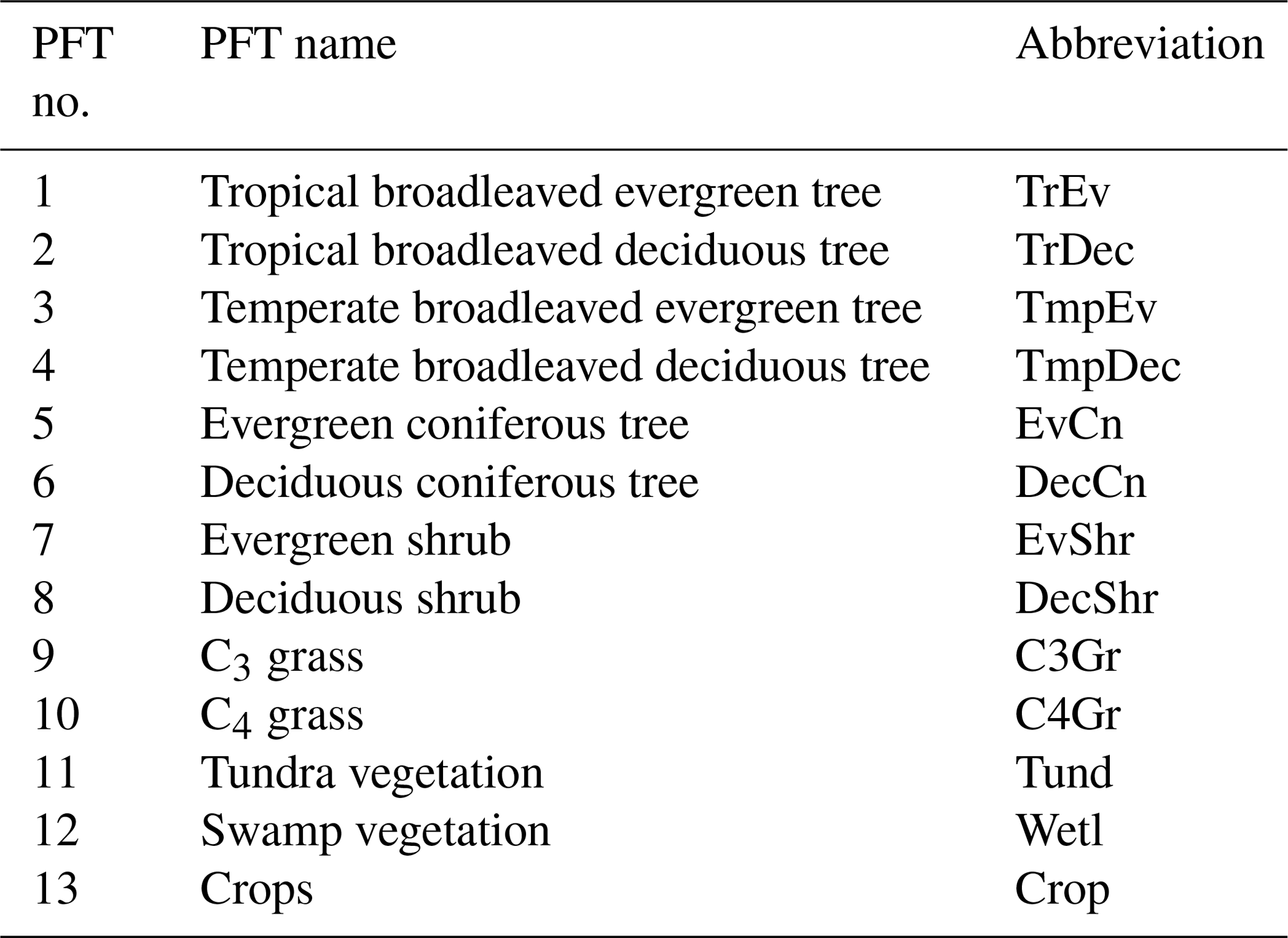
We use the OCO-2 processed SIF-lite data files. For details on the retrieval algorithm for the SIF data see Frankenberg et al. (2014) and Sun et al. (2018). These data are gridded at 2∘ × 2∘ spatial resolution, equivalent to the model grid resolution. We exclude soundings collected over water as determined by the corresponding International Geosphere-Biosphere Programme (IGBP) land classification index (Friedl et al., 2010). We use instantaneous SIF at 757 nm and only soundings taken in nadir mode. Data are also available at 771 nm; however, the signal at 757 nm is stronger (Sun et al., 2018), and thus we only consider that signal. The annual mean OCO-2 SIF for 2015 is shown in Fig. 1.
There are potential limitations in using OCO-2 for global mapping due to spatial coverage of the observations and sampling bias of biomes, particularly if it differs from the assumed biome types used in the model. We assessed the similarity between the sampled IGBP land classification index of the OCO-2 soundings and the BETHY-SCOPE PFTs to evaluate this limitation. Considering the differences in vegetation classifications this is a qualitative test. Qualitatively, the occurrence of IGBP biome sampling appears to be similar to the BETHY-SCOPE PFTs. Moreover, Frankenberg et al. (2014) showed that despite the limited spatial coverage of OCO-2 it provides a representative sampling of 1∘ × 1∘ grid cell averages. We therefore do not perform any further filtering of the data. Future studies may benefit from evaluating this in more detail and performing the assimilation using observations at a PFT-specific level rather than the grid cell level as is applied here.
Observational uncertainty
The calculation of observational uncertainties is an important aspect of any data assimilation study as it partly determines posterior probabilities. We note two rather extreme cases in calculating the uncertainty in the satellite observations of SIF. The first is to take the average of the single measurement precision error, considered an overestimate of the uncertainty as it does not account for the sample size. Second is to calculate the standard error, where the average of the single measurement precision error is divided by the square root of the number of observations, as applied in Parazoo et al. (2014). Use of the standard error almost certainly underestimates the uncertainty as it neglects correlated or systematic errors.
Therefore, to determine the measurement error of SIF (σ) in a given grid cell (i), we sum the single measurement precision error (σe) of each sounding within that grid cell and divide by the total number of soundings (ni). Dividing this by one half scales it closer to the standard error but remains a conservative estimate of the actual error.
Calculated uncertainties are shown for January and July 2015 in the Supplement, in Figs. S1 and S2. Statistical tests on the results, using the so-called reduced chi-squared statistic, allow us to test whether these observational uncertainties are consistent with other aspects of this data assimilation process, as outlined further below.
2.4 Data assimilation system
To assimilate SIF into BETHY-SCOPE we require a minimization algorithm, cost function and error propagation method. A variety of techniques are available for the optimization of terrestrial biosphere models and reviews are available (Fox et al., 2009; Kaminski et al., 2013; MacBean et al., 2016; Trudinger et al., 2007).
We utilize a probabilistic framework whereby quantities (e.g., observations, model state variables, model process parameters) are represented by their PDF. These quantities are treated as Gaussian, and thus can be described by their mean and standard deviation. For the model parameters the mean is denoted by x and error covariance matrix by Cx. We denote the prior parameter vector and covariance matrix by x0 and , respectively, and the posterior parameter vector and covariance matrix by xpost and , respectively. For the observations the mean is denoted by d. The error covariance matrix in observation space, denoted by Cd, combines errors in the observations and in their simulated counterpart, i.e., model (Kuppel et al., 2013). Quantification of model error can be performed through an assessment of model–observation residuals following optimization (e.g., Kuppel et al., 2013). We assess potential model errors in this study; however, we do not explicitly account for this error in the propagation of errors onto GPP; hence Cd accounts only for errors in the observations. We point out that the uncertainty is embodied in the error covariance matrices and that diagonal elements represent the variance of the quantities while off-diagonal elements represent error covariances between quantities.
2.4.1 Assimilation procedure
The assimilation procedure finds the posterior PDF for the target variables which, in this case, are the model process parameters. We assume Gaussian PDFs, so our posterior PDF is described by its mean and standard deviation. The mean is also the maximum posterior estimate which can be found by minimizing a cost function (J). The cost function, shown in Eq. (5), quantifies the difference between the model simulated SIF (M(xn)) and SIF observations (d) and the departure of parameter values (xn) from the prior estimate (x0). These differences are squared and normalized by the uncertainties in the observations Cd and model parameters Cx, respectively, allowing for more certain quantities to carry more weight. J thus provides a measure of the model-observed mismatch and the deviation from the prior information accounting for uncertainties. We consider the optimization to have converged on an optimal solution when the change in the cost function is less than 1 % of the change that occurred during the first iteration.
To find the minimum of J we employ a quasi-Newton's method, which is a variational, iterative technique (p. 69 Tarantola, 2005). This algorithm requires a matrix of partial derivatives of the observable with respect to model parameters, called the Jacobian matrix (H), calculated using finite differences. H is therefore a representation of the sensitivity of model-simulated SIF to each model parameter.
The quasi-Newton algorithm assumes weak nonlinearity in the model. This approximation is better than assuming a linear model, but not as useful as having a model adjoint where the entire parameter space can be efficiently examined (Kaminski et al., 2013). With this assumption the model is presumed to be linear about the point where H is calculated. However, to account for nonlinearities in the model we recalculate H after each iteration of the algorithm. Given a single “global” minimum of J, this algorithm will converge upon it (Tarantola, 2005). There is still potential that the algorithm will converge upon a local minimum in J.
For each iteration n of the algorithm the parameter vector (xn) is updated using Eq. (6). This adjusts for nonlinearity by performing a forward run of the full nonlinear model at each iteration (M(xn)). It takes the following form:
where μ is a step-size (set to 0.2) as required in gradient-based techniques (Tarantola, 2005). In a case where the parameter update produces values that are unphysical (e.g., negative Cab), they are reset to the nearest physical value for the next iteration.
Alongside J the reduced chi-squared () statistic is used to assess the match with the observations. Shown in Eq. (7) below, measures the goodness of fit per observation accounting for observational uncertainties, where N is the number of degrees of freedom which is equal to the total number of observations in our case.
Under the Gaussian assumption this widely applied statistical test assesses the appropriateness of our assumed uncertainties. With a value of 1 the statistical assumptions that underlie our procedure, including the assumed errors, are consistent with the model–data mismatch (see Tarantola, 1987, p. 212). This means the fit to the data is as good as the assumed distributions say it should be. Informally, this would mean we are neither over-fitting or under-fitting the data.
2.4.2 Error estimation
For linear and weakly nonlinear problems Gaussian probability densities propagate forward through to Gaussian distributed quantities (Tarantola, 2005), termed linear error propagation. The posterior parameter errors, , are estimated using linear error propagation as shown in Eq. (8) as follows:
where H is calculated at the posterior (i.e., xpost). Rayner et al. (2005) demonstrated how to propagate these parameter uncertainties forward through a model onto simulated quantities such as carbon fluxes. Using the Jacobian rule for probabilities, parameter uncertainties in the model parameter covariance matrix ( and ) can propagate forward onto GPP using Eq. (9): this determines the error covariance of GPP (CGPP).
where HGPP is the model Jacobian with respect to GPP. To calculate the prior error covariance of GPP, HGPP is calculated about the prior parameter vector and Cx equals . To calculate the posterior error covariance of GPP, HGPP is calculated about the posterior parameter vector and Cx equals . The difference between these two cases determines the change in GPP error covariance and therefore the uncertainty reduction in GPP.
2.5 Experimental setup
In this study BETHY-SCOPE is run for the year 2015. This constitutes the optimization (or calibration) period. We then assess the optimized model performance against independent OCO-2 observations outside of the optimization period from September to December 2014.
The model is run on a 2∘ × 2∘ grid resolution. Climate forcing data are provided in the form of monthly meteorology (precipitation, minimum and maximum temperatures, and incoming solar radiation) obtained from the WATCH/ERA Interim dataset (WFDEI; Weedon et al., 2014). These are used to derive average diurnal cycles of meteorological forcing. Thus, a single average diurnal cycle of meteorological forcing for each month is used to simulate photosynthesis and fluorescence. This allows the computation of SIF at the equivalent overpass time as the satellite data (13:00–14:00 local time). The model SIF is also calculated at the equivalent wavelength to the OCO-2 SIF data (757 nm). Atmospheric CO2 concentration is set to the 2015 annual average. LAI is prescribed to the model using the MODIS improved LAI dataset (Yuan et al., 2011). The LAI is averaged at the model 2∘ × 2∘ grid resolution and for each grid cell it is split between PFTs using the model PFT grid cell fractional coverage.
2.6 Global GPP products for comparison
To assess the SIF-optimized global GPP we compare the model prior and posterior GPP to other global GPP products. The first dataset for comparison is an upscaled product based on site-level measurements termed FLUXCOM GPP (Tramontana et al., 2016). The FLUXCOM GPP product uses various machine-learning techniques to empirically upscale flux tower data using remote sensing and meteorological data as the predictor variables. Here, we use the ensemble average of the FLUXCOM GPP product that uses remote sensing data exclusively (Tramontana et al., 2016). The second dataset for comparison is an ensemble of 11 global dynamic vegetation models forced with equivalent climate fields and atmospheric CO2 concentration that were used to investigate trends in sources and sinks of CO2 (TRENDY; Sitch et al., 2015). It is important to note that global GPP is highly uncertain and that both the FLUXCOM GPP and TRENDY GPP estimates are based on their own model assumptions and/or sparse measured data (Anav et al., 2015). Therefore, these data are used to evaluate whether the SIF assimilation results in global patterns of GPP that align with the current understanding and not for extensive validation purposes.
There is an abundance of results that may be presented from a global data assimilation study with SIF. First, we present the model fit to the observed SIF for the prior and posterior cases and for the calibration and validation periods. Second, we examine the estimated parameters and their associated uncertainties. Third, we present the spatiotemporal patterns of model GPP alongside other model GPP products. Finally, we present derived quantities from the model including APAR and photosynthetic light-use efficiency.
3.1 Assimilation with SIF
Here we show how the model compares with the observed SIF (shown in Fig. 1) for the prior and posterior cases and for the calibration and validation periods. The goodness of fit between modeled and observed SIF is assessed using multiple metrics. The fit is a key metric (see Eq. 7). Differences between the model and observations (“residual”) and the squared residual normalized by the observational variance (“mismatch”) are also used. The mismatch is a measure of the difference between the model and observations accounting for observational uncertainties, indicating the contribution grid cells make toward the cost function. The model fit during the calibration period is presented in more detail as there is more data. The model fit during the validation period provides a more stringent test of the assimilation performance. We then show the performance of an additional model simulation testing seasonal variation in parameters.
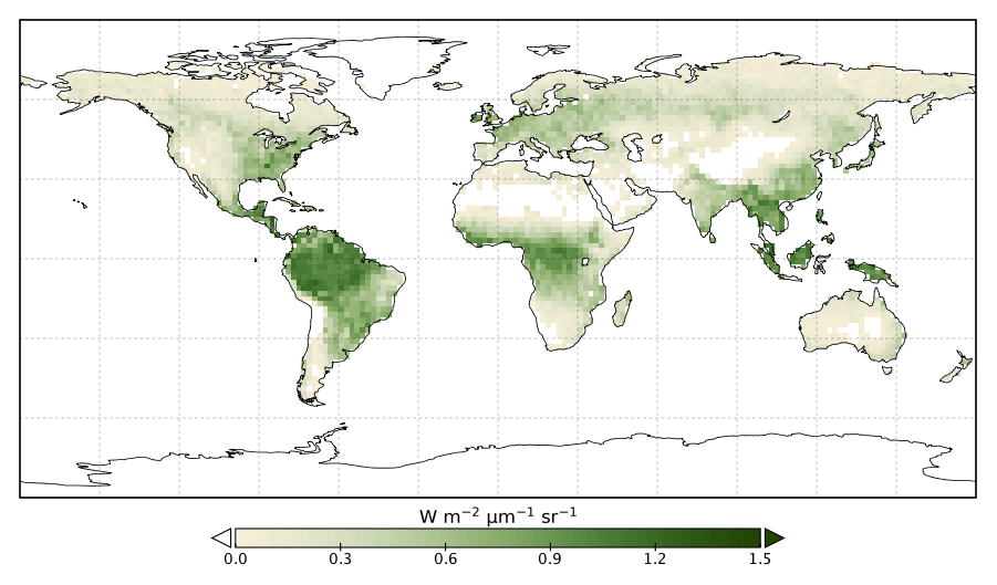
Figure 1Annual mean observed SIF from the OCO-2 satellite for 2015.
3.1.1 Calibration
The model prior SIF (SIFprior) over the calibration period yields a global fit of 2.45. Large residuals in the annual mean, shown in Fig. 2, are evident across the globe, ranging from −0.87 to +1.20 . Generally, SIFprior overestimates observed SIF across regions dominated by tropical forest (e.g., the Amazon, western equatorial Africa and Maritime Continent), boreal forest (parts of North America and Eurasia) and semiarid regions (e.g., central Australia, central Asia and southern Africa). SIFprior tends to underestimate observed SIF across the rest of the land, in particular for regions dominated by croplands (e.g., American Midwest, parts of Europe, India, eastern Asia), mixed forests (across Europe and Asia), and grassland and savanna regions (e.g., the African savanna and Brazilian Highlands of South America). Latitudinal averages, shown in Fig. 4, also show these spatial patterns for SIFprior. Overestimation of observed SIF is seen over the central tropics between 15∘ S and 5∘ N, a region dominated by tropical evergreen forest (TrEv), whereas there is significant underestimation of observed SIF over the Northern Hemisphere, particularly during northern summer (see Fig. 5).
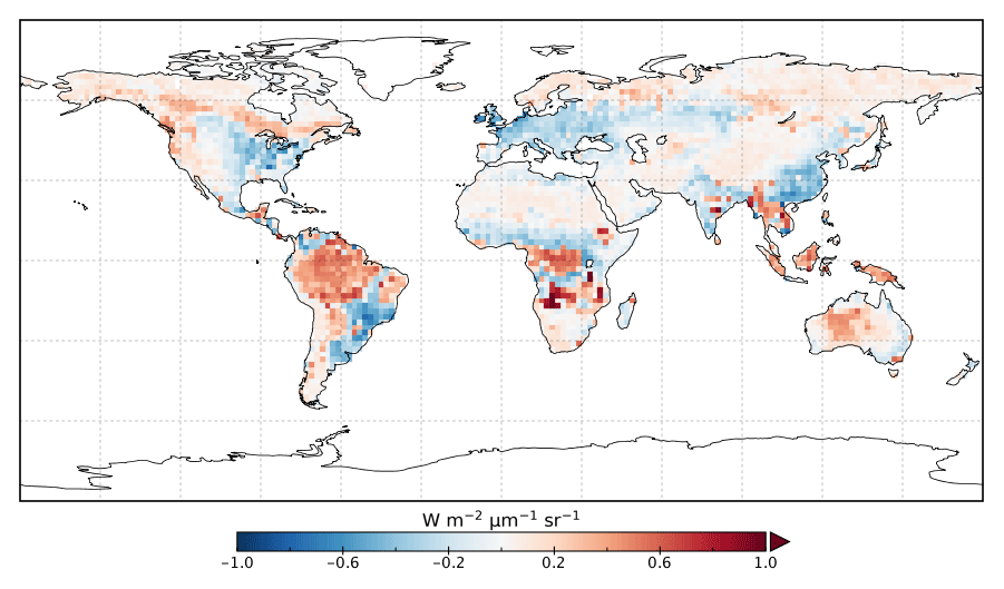
Figure 2Annual mean residual between model SIFprior and observed SIF for 2015.
Figure 3Annual mean residual between model SIFpost and observed SIF for 2015.
Following the assimilation, the model shows a considerably better fit to the calibration data. The global fit is strongly reduced from 2.45 to 1.01. This is close to the optimal value of 1, demonstrating the ability of the optimized model to fit the observed patterns of SIF and validating our chosen uncertainties as far as is practicable, including the choice of the scaling used to calculate observational uncertainties in Eq. (4). Annual mean residuals between model posterior SIF (SIFpost) and the observations, shown in Fig. 3, range between −0.58 and +0.45 , considerably smaller than SIFprior. The spatial patterns of posterior residuals (Fig. 3) show that the regional patterns of residuals broadly exhibit the same sign as the prior case albeit with a significantly reduced magnitude. For the latitudinal averages, SIFpost is remarkably close to the observed SIF for the annual average (Fig. 4). However, discrepancies are evident for the northern summer averages for both SIFprior and SIFpost (Fig. 5), where observed SIF is underestimated in the Northern Hemisphere and overestimated in the Southern Hemisphere.
Latitudinal sums of the mismatch between the model and the observations (bar charts in Figs. 4 and 5) also show a significant reduction (i.e., improvement in fit) following the assimilation. Comparison of the gray and green bars, indicating the respective prior and posterior mismatch, show that this improvement in fit occurs over all latitudes at the annual and northern summer timescales. The total annual mismatch between SIFpost and the observations is about 40 %–80 % smaller across the latitudes between 40∘ S and 60∘ N relative to SIFprior.
Despite the strong improvement in fit, SIFpost tends to underestimate large observed SIF values >1.0 , shown in the Fig. S4. A linear regression line between the observed SIF and SIFpost has a slope of 0.67. Furthermore, while the observed SIF for any given month and grid cell can reach up to 2.29 , SIFprior does not exceed 1.98 and SIFpost does not exceed 1.43 . The SIFprior does not show this systematic underestimation, however, but it has a poorer global fit (Fig. S3). We note that these large observed SIF values occur mostly over the tropics and the northern midlatitudes during the peak growing season.
From Fig. 3 it appears that SIFpost overestimates observed SIF over arid regions (e.g., the Sahara, Atacama and Namib deserts, central Australia and central Asia). This occurs primarily because the observed SIF is slightly negative (see Fig. 1), potentially due to measurement noise or issues from the correction of constant error artifacts in the SIF retrieval (Sun et al., 2018). Negative SIF values are still considered in the assimilation system. However, they contribute little to the overall mismatch given the uncertainty in the SIF observations (see Figs. S8 and S9).

Figure 4Latitudinal averaged SIF and mismatch with observations. OCO-2 observations (black line), SIFprior (gray dashed line, gray bars) and SIFpost (green line, green bars) for the annual average. Data are only shown for spatiotemporal points where OCO-2 observations are present.

Figure 5Latitudinal averaged SIF and mismatch with observations. OCO-2 observations (black line), SIFprior (gray dashed line, gray bars) and SIFpost (green line, green bars) for northern summer (June–August). Data are only shown for spatiotemporal points where OCO-2 observations are present.
3.1.2 Validation
To validate the optimized model we assess the model fit to independent OCO-2 SIF data from September to December 2014, outside of the calibration period. The global for SIFprior is 2.57, while SIFpost is 1.06 (Figs. S5 and S6). This indicates a strong improvement in fit following the SIF assimilation. Comparison of SIFpost with the validation data shows that large SIF values (> 1.0 ) are systematically underestimated, similar to the fit to calibration data. For these validation data, these large SIF values typically occur over tropical forest, grassland and cropland regions.
3.1.3 A case with seasonally varying parameters
Most terrestrial biosphere models assume process parameters are constant through time despite evidence showing that some of these biophysical variables (e.g., Cab, Vcmax) vary in response to resource availability (e.g., Demarez, 1999; Wang et al., 2007; Wilson et al., 2000; Xu and Baldocchi, 2003; Zhang et al., 2014). At present the BETHY-SCOPE model does not include any mechanism for varying these with time, other than a temperature correction for Vcmax. Given this, we expect that assuming these parameters are temporally constant will contribute to the disparity between the modeled and observed SIF, particularly for more seasonal vegetation.
Thus, an additional comparison is made where we apply a simple seasonal cycle to Cab and Vcmax parameters for the posterior model. We set the annual mean to be the posterior Cab and Vcmax values and apply a seasonal cycle by using a sine function that has a period of 1 year, a maximum on the summer solstice (i.e., 22 December in the Southern Hemisphere and 22 June in the Northern Hemisphere) and an assigned amplitude (see Eqs. S1 and S2 in the Supplement). For highly seasonal PFTs including deciduous trees and shrubs, C3 and C4 grasses, and crops, the amplitude is set to 50 % of the mean, while for all other PFTs the amplitude is set to 10 %. While this seasonal cycle is arguably oversimplified, this still provides us with a simple sensitivity test to investigate whether introducing a more formal seasonal variation in Cab and Vcmax would improve the fit with the observed SIF.
Implementation of seasonally varying Cab and Vcmax results in a moderate improvement in fit with the observed SIF (Fig. S7). The posterior fit improves from 1.01 to 0.91 given the seasonally variable parameters (SIFpost,seas). Both the coefficient of determination (R2) and slope of a linear regression line improve with SIFpost,seas, with R2 increasing from 0.74 to 0.77 and the slope increasing from 0.67 to 0.71 (Fig. S7). This indicates that the systematic underestimation of large observed SIF values may be improved. Furthermore, the fit to the observed SIF data >1.0 shows a strong improvement given seasonally varying parameters, going from 3.97 for SIFpost to 2.99 for SIFpost,seas. The fit to low SIF values (<0.25 ) also improves from 0.56 for SIFpost to 0.50 for SIFpost,seas. Notably, when the fit is assessed per PFT (i.e., grid cells with the same spatially dominant PFT are considered together) the fit improves for all of these “biomes”.
3.1.4 Fit to the seasonal cycle
We can also assess the seasonal cycle of SIF to determine how well the model simulates the amplitude of observed SIF. First, we assess how well the model replicates the seasonal amplitude of observed SIF across all spatial points. Second, we assess the seasonal patterns of SIF for a selection of case study regions in more detail. We avoid assessing the seasonal cycle of SIF aggregated at global or hemispheric scales as regional patterns of residuals can differ in sign and magnitude (e.g., see Fig. 3). The seasonal amplitude of observed SIF is calculated as the difference between the maximum and minimum SIF across the year for each grid point. To increase confidence that the observations really capture the seasonal cycle, we only assess grid points with at least 8 months of observed SIF data. In doing so, most regions north of 60∘ N are excluded due to limited SIF observations. We do not assess the timing of the seasonal cycle (e.g., start and end of the growing season) as this is largely driven by LAI which is prescribed and therefore fixed in this study.
The comparison of the seasonal amplitude of observed SIF against SIFprior, SIFpost and SIFpost,seas is shown in Fig. S10. The model underestimates the observed seasonal amplitude in all cases. With a perfect match to the observed seasonal amplitude the model would follow the 1:1 line and the slope of a linear regression line would equal 1. However, we find that the slope is 0.21 for SIFprior, 0.35 for SIFpost and 0.43 for SIFpost,seas. Spatial points with the largest seasonal variations in observed SIF also exhibit the largest model-observed mismatch (Fig. 6).
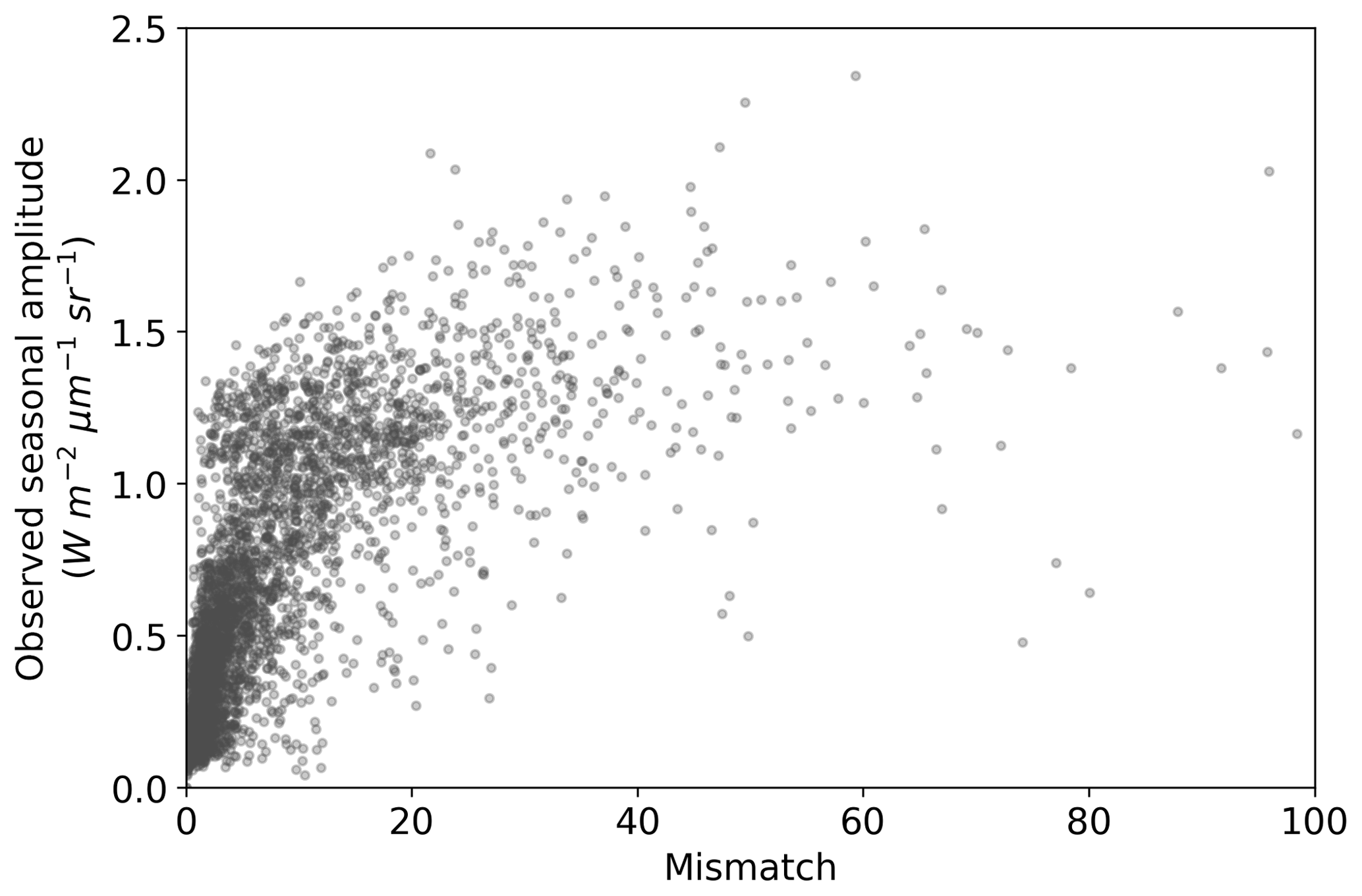
Figure 6Seasonal amplitude of observed SIF versus the model-observed mismatch for the SIF optimized (SIFpost) model. Mismatch is defined as the squared residual normalized by the observational uncertainty (expressed as variances). A positive curvi-linear relationship exists such that spatiotemporal points with a large model-observed mismatch generally also exhibit a large observed seasonal amplitude.
For a more detailed assessment of seasonal patterns we investigate three case study regions: (i) the tropical forest of mainland southeast Asia, (ii) croplands in North America and (iii) the north African savanna (see Figs. S11–S15 for details). These regions are selected as they represent quite different biome types, exhibit varied SIF patterns and have relatively large posterior model-observed mismatch.
The tropical evergreen forest of mainland southeast Asia exhibits a clear seasonal cycle in observed SIF. The monthly mean observed SIF averaged over this region varies from a minimum of ∼0.6 in March to a maximum of ∼1.4 in August (see Fig. S11). Both SIFprior and SIFpost exhibit seasonal cycles that differ strongly from the observations, with little change in the shape of the seasonal cycle from the prior to posterior simulations. Model SIF shows a minimum in July and two maximums in February and November, following the seasonal evolution of LAI (see Fig. S11), which we reiterate is prescribed. This results in strong negative temporal correlations between observed SIF and model SIF as over this region.
Croplands in North America are heavily managed landscapes with highly productive vegetation as indicated by the large observed SIF values during the growing season. Even with the monthly averages used here, observed SIF can exceed 2.0 . As presented earlier, the model SIF cannot match the seasonal amplitude of observed SIF and subsequently underestimates the maximum monthly SIF averaged over this region by almost 40 % (0.45 ) (see Fig. S13). The fit is improved in SIFpost,seas (; ). In both cases the timing of seasonal maximum and senescence is simulated quite well, while the onset of the growing season is predicted to be too early.
The north African savanna exhibits a strong seasonal cycle in observed SIF. This region is dominated by grasslands and open forest, with a seasonality closely following the seasonal variation in precipitation. Averaged over the region, observed SIF varies from 0.07 in January to 0.77 in September (see Fig. S15). However, SIFpost exhibits a much smaller seasonality with variation from 0.24 to 0.48 across the year, only 34 % of the observed seasonal amplitude. Temporal correlations are quite strong, however, as model SIF also reaches its peak in September.
3.2 Estimated parameters
The prior and posterior parameter mean values and associated uncertainties are shown in Table A1. In this data assimilation system the number of observations far outweighs the number of unknowns. This means that there is a substantial amount of observational information available to constrain parameter values, and thus they can shift from their prior values considerably even if given a relatively tight prior uncertainty. We can be more confident in parameters that see large reductions in uncertainty. Conversely, parameters with little reduction in uncertainty following optimization should be accepted cautiously.
Posterior Vcmax estimates range from 16 to 130 . The lowest posterior rates occur for the TmpEv, C4Gr, Tund and Wetl PFTs, all equal or below 30 . The highest posterior rates occur for the Crop and C3Gr PFTs, both exceeding 100 . Out of 13 PFTs, 9 see an increase in Vcmax. Increases greater than 2 standard deviations occur for the PFTs TmpDec, EvCn, C3Gr, C4Gr and Tund, many of which dominate temperate regions. Latitudinal averages of Vcmax (Fig. S19) show a strong increase in temperate-zone Vcmax following the SIF assimilation, shifting it higher than Vcmax in the tropics. Zonally, the lowest Vcmax occurs in the cold-climate high latitudes. Most of these parameters see moderately strong uncertainty reductions (>30 %), indicating strong constraints from SIF.
Posterior Cab estimates range from 8 to 38 µg cm−2. Out of 13 PFTs, 9 see a decrease in Cab. The highest posterior Cab values occur for the TrEv, TmpEv, TmpDec, DecCn and Crop PFTs, all >25 µg cm−2, while the lowest values occur for the EvShr, Tund and Wetl PFTs, all <15 µg cm−2. Uncertainty reduction ranges from weak to moderately strong for the Cab parameters, with a maximum constraint of 34 %. Latitudinal averages of posterior Cab show a relatively low variance across different zones (Fig. S20), with posterior values being similar between the tropics and temperate midlatitudes, albeit with a distinct dip in drier subtropics and high latitudes. The leaf composition parameter for dry matter content, Cdm, increases by about 70 % and an uncertainty reduction of about 20 %. The leaf composition parameter for senescent material remains almost unchanged and shows only a very weak uncertainty reduction of about 1 %.
Parameters that control canopy structure and the leaf angle distribution see large deviations from their prior values. Some leaf angle distribution parameters, LIDFa and LIDFb, shift considerably. SIF is particularly sensitive to the LIDFa and LIDFb parameters, although this depends on which group of PFTs they pertain to, and so these parameters have uncertainty reductions of up to 90 %. Vegetation height for both trees and shrubs remain relatively unchanged, while vegetation height for grasses and crops see a decrease of over 4 standard deviations. However, the uncertainty reduction of the vegetation height parameters is very weak (<1 %). Despite these changes GPP is relatively insensitive to the canopy structure parameters.
3.3 Estimated GPP
The spatial patterns of posterior GPP and the changes following the SIF assimilation are shown in Figs. 7–11. Following the assimilation of SIF global GPP increases by about 39 Pg C yr−1, from 127.6 to 166.7 Pg C yr−1. This change shifts BETHY-SCOPE further from the TRENDY mean (142.4 Pg C yr−1) and FLUXCOM GPP (103.3 Pg C yr−1) estimates. The parametric uncertainty in global GPP is reduced by 38 % from ±7.4 to ±4.6 Pg C yr−1 by the SIF assimilation.
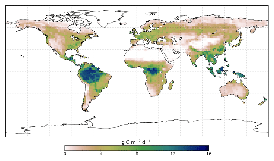
Figure 7Spatial patterns of BETHY-SCOPE posterior annual mean GPP (GPPpost) for 2015.
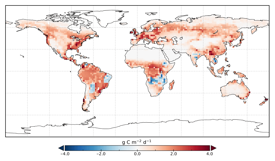
Figure 8Change in annual mean GPP rate for 2015 following optimization with SIF relative to GPPprior.
Spatially, increases in annual GPP are seen across much of the land surface as shown in Fig. 8 (see Fig. S17 for the percentage change in GPP). Declines in GPP are seen in dry tropical forests in parts of South America, Africa and mainland Asia (TrDec PFT; also shown in Fig. 9). Globally, TrDec-dominated forests see a decline in total GPP of 23 %. Two other biomes, TmpEv and DecShr, show a decline in global GPP; however, their contribution to global GPP is relatively small (see Fig. 9). The global GPP of TrEv forest biomes, including the Amazon, equatorial Africa and Maritime Continent, increase by about 20 %. In relative terms, the largest increases in global GPP occur for TmpDec, EvCn, C3Gr and C4Gr, all >60 %. We note that these changes in model GPP can differ in sign and magnitude from the changes in model SIF (see Figs. 8 and S18). This can occur as SIF and GPP have differing sensitivities to the underlying parameters, a result of the process-based approach. For example, the wet tropical forests (TrEv) and cold-climate conifer forests (EvCn) see an increase in GPP but decline in SIF.

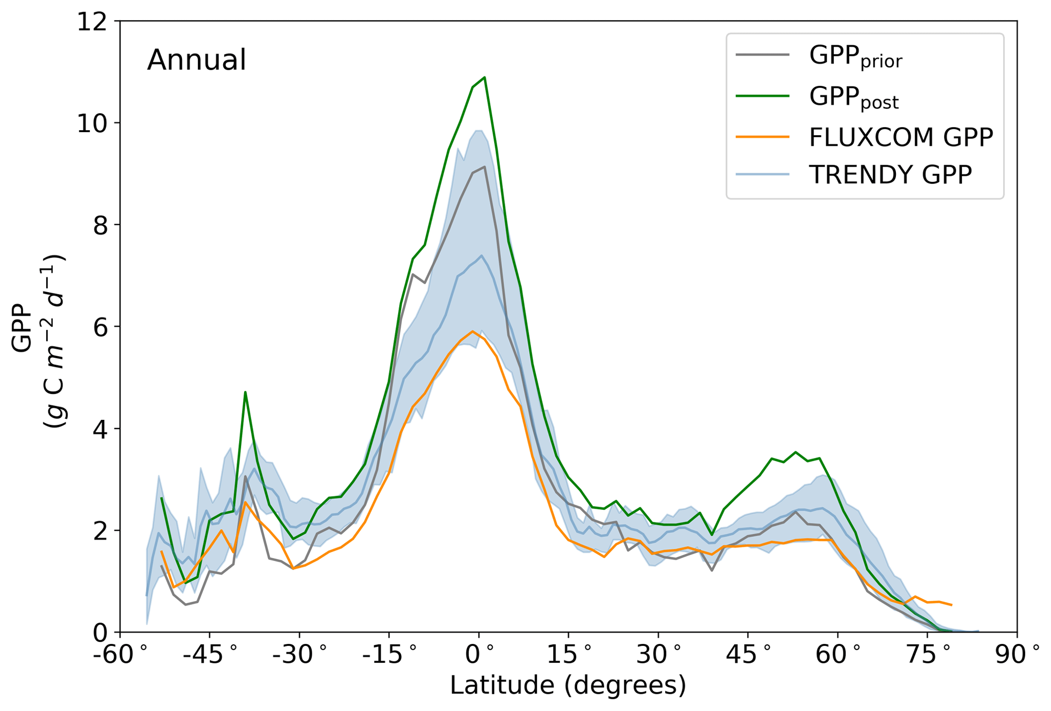
Figure 10Annual latitudinal averages of GPPprior (gray line), GPPpost (green line), FLUXCOM GPP (orange line), TRENDY model average (light blue line) and TRENDY model spread given by the 10th and 90th percentiles (light blue shading).
Averaged over latitudinal bands (Figs. 10 and 11) we can see the distinctive peak in GPP across the tropics at the annual timescale and secondary peak in GPP across the northern midlatitudes during the northern summer. With the assimilation of SIF the GPP across all latitudes increases. Some regions and seasons see larger changes. Across the central tropics (15∘ S–5∘ N; dominated by the PFT TrEv), GPP increases substantially. For this region, the prior and posterior estimates are near the high end of other estimates, with the posterior GPP exceeding the 90th percentile of TRENDY models (blue shading). FLUXCOM GPP is very low in the central tropics, but we note that this product is not expected to be representative of the tropics given the sparsity of the flux tower network there (Tramontana et al., 2016). The northern extratropics (30–60∘ N) show a general increase in BETHY-SCOPE GPP, with the SIF assimilation shifting it to the higher end of other estimates. This is particularly strong during northern summer (Fig. 11). While the prior GPP in this region is within the TRENDY model range and close to the FLUXCOM GPP, the SIF assimilation results in a posterior that exceeds the 90th percentile of the TRENDY model range. North of 65∘ N the prior closely matches FLUXCOM GPP, but the posterior sees an increase which brings it more in line with the TRENDY model average. There is also a distinct difference between the FLUXCOM GPP product and all models north of 75∘ N, with FLUXCOM GPP being higher. BETHY-SCOPE posterior GPP over the southern latitudes south of 15∘ S is generally within the TRENDY model range. In this region, the prior GPP is near the bottom of the TRENDY model range, although this shows closer similarity to the FLUXCOM GPP.
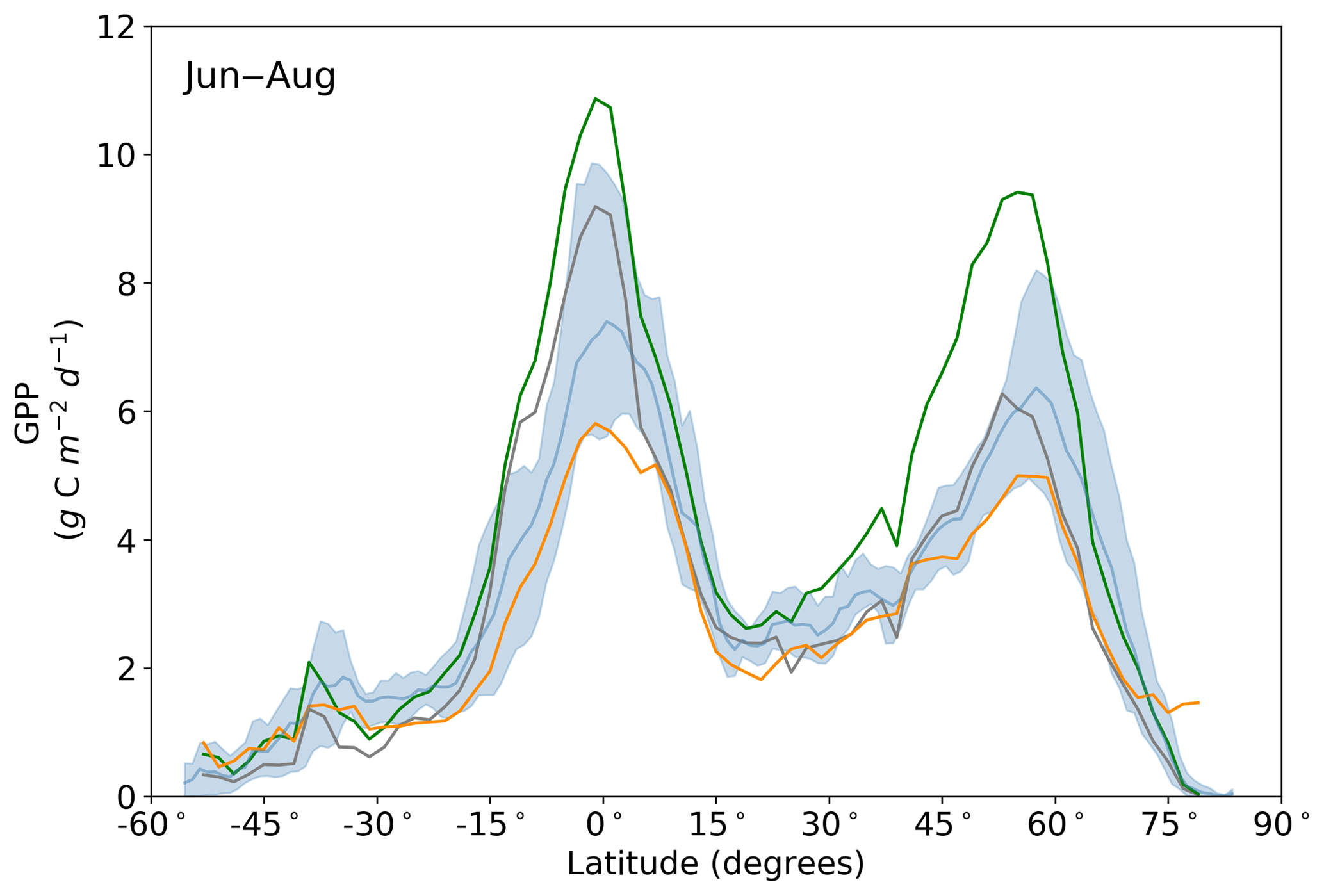
Figure 11Northern summer (June–August) latitudinal averages of GPPprior (gray line), GPPpost (green line), FLUXCOM GPP (orange line), TRENDY model average (light blue line) and TRENDY model spread given by the 10th and 90th percentiles (light blue shading).
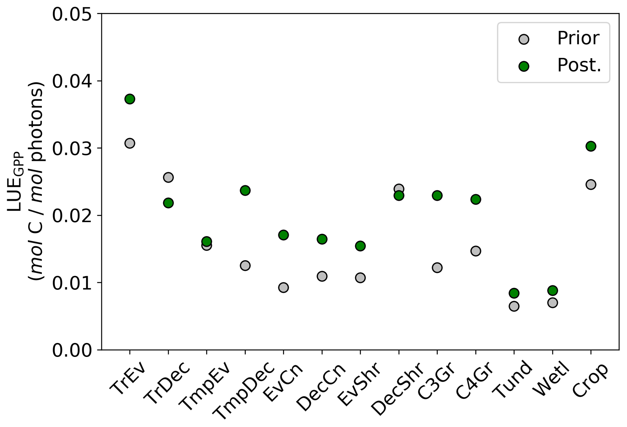
Figure 12Per PFT LUEGPP for the prior and posterior simulations. Values were determined by monthly average GPP divided by monthly averaged APAR, then averaged to annual scales thus averaging over seasonal variations. Note that the theoretical maximum is 0.08 mol C mol photons−1 (Waring et al., 2016).
A useful metric for patterns of global productivity is the ratio of GPP between different regions. These ratios are summarized in Table B1 in Appendix B. The ratio of the tropics (30∘ S–30∘ N) to the extratropics (south of 30∘ S and north of 30∘ N) declines following the SIF assimilation, due to a relatively larger increase in extratropical GPP compared to tropical GPP. This shifts the ratio of tropical to extratropical GPP from a prior of 2.47 to a posterior of 1.94, which is substantially closer to patterns of the FLUXCOM (1.90) and TRENDY (1.93) mean. Similarly, the ratios of the tropics to the boreal region (north of 55∘ N), tropics to the temperate region (south of 30∘ S and north of 30–55∘ N) and the temperate to boreal region converge toward the FLUXCOM values (see Table B1).
We also note an improvement in the correlation between the BETHY-SCOPE estimate and the FLUXCOM GPP over North America (see Figs. B1 and B2 in Appendix B) and Europe (data not shown), two regions where FLUXCOM GPP has considerably more training data. Over North America the correlation improves from a prior R2=0.80 to a posterior of R2=0.89, while over Europe the correlation improves from a prior R2=0.76 to a posterior of R2=0.86. Despite this improvement in match between the patterns, the posterior slope is 1.6 for North America and 1.8 for Europe, indicating that the magnitude of posterior monthly GPP is larger than that of FLUXCOM GPP.
Changes in GPP due to changes in parameter values can be broken down into changes in intercepted radiation (APAR) and canopy photosynthetic light-use efficiency (LUEGPP). The LUEGPP is calculated as the annual average of the ratio between monthly GPP to monthly APAR. Overall, the majority of biomes see an increase in LUEGPP following the SIF assimilation, shown in Fig. 12. Just three biomes, TrDec, TmpEv and DecShr, see a decline in LUEGPP. These biomes are the same that see a decline in annual GPP (comparing Figs. 8 and B4). This can be related back to the general increase in Vcmax for most PFTs (Table A1) and latitudes (Fig. S19). Changes in APAR are smaller in relative terms and show distinct regional differences (Fig. B6). With the exception of low-productivity arid regions, the largest percentage change in APAR occurs for the high-latitude tundra biome with approximately a 20 % increase in APAR, due primarily to an increase in Cab. Wet tropical forests see a decline in APAR of about 5 %, while drier tropical biomes (e.g., Brazilian Highlands, north African savanna) see an increase of <5 %. Other regions show only minor shifts in APAR.
The use of satellite-derived SIF in a data assimilation system has substantially improved the performance of the BETHY-SCOPE model against calibration and validation SIF observations. The posterior model fit is similarly good between the validation period () and calibration period (), indicating that the model performs similarly well outside of the assimilation period. We show that with the inclusion of seasonal variations in biophysical quantities (e.g., Cab and Vcmax) the fit to SIF can be improved further as well as provide a better representation of ecosystem function. We highlight that the improvement in fit following the assimilation occurs given equivalent LAI fields. Overall, assessing the optimized model in this way is a key validation test and highlights the improvement following the assimilation. While this is the most stringent validation we can carry out with the available data (considering the available OCO-2 and model meteorological forcing data), future work should consider longer periods to sample more varied climatic conditions. Assessment against other satellite SIF products (e.g., GOME-2, GOSAT, TROPOMI) is also feasible provided that careful consideration is taken of the instrumental differences.
The SIF-optimized model produces a global GPP of 166.7 Pg C yr−1 for 2015. This is an increase of 31 % relative to the prior and is due to increases in GPP in both tropical and extratropical regions. Other approaches to quantify GPP globally have produced a large range of estimates over different periods including 119 Pg C yr−1 (Jung et al., 2011), 146 Pg C yr−1 (Koffi et al., 2012), 157 Pg C yr−1 (Peylin et al., 2016) and 175 Pg C yr−1 (Welp et al., 2011). As pointed out by a recent review of global GPP (Anav et al., 2015), validating GPP estimates at these large scales is highly challenging. Nevertheless, the substantial improvement in fit with SIF data during the calibration and validation periods provides some confidence in the overall spatial patterns (Figs. 4, 5, S3–S6). Indeed, the correlation of BETHY-SCOPE GPP with the FLUXCOM GPP over North America and Europe, regions with many calibration sites, improves with the assimilation of SIF observations despite showing a higher magnitude. This suggests that the SIF assimilation brings about better agreement on the spatial patterns but disagreement on the magnitude. While there is no wholly measurement-based GPP with which to validate our GPP estimate (Anav et al., 2015), there is some recent evidence that is consistent with the results that the productivity of the northern midlatitudes may be higher than previously thought. Badgley et al. (2018), for example, used measurements of near-infrared reflectance of vegetation (NIRv) and flux tower data to upscale GPP, producing a higher GPP in midlatitude ecosystems than the FLUXCOM product. This occurred even though the two methods have similar predictive capabilities of flux tower GPP (Tramontana et al., 2016). Furthermore, evidence from SIF-based estimates of cropland GPP, such as the American Midwest, produce GPP that is 50 %–75 % higher than most models predict (Guanter et al., 2014). Further analysis is required to assess if this is consistent with other measured data such as carbonyl sulfide, another proxy for GPP (Campbell et al., 2008).
The SIF assimilation also alters the distribution of global GPP. Here, we find that extratropical ecosystems contribute relatively more to global productivity with the SIF assimilation. Despite an increase in the GPP rate over the tropics, their relative contribution reduces from 71 % to 66 % of global productivity (see Table B1). This result differs from both MacBean et al. (2018) and Parazoo et al. (2014), as they found relatively larger increases in tropical GPP such that tropical ecosystems contributed more to global productivity following the assimilation of SIF data. Nevertheless, it is difficult to reconcile the relative and absolute changes in GPP across these studies.
Perhaps the largest difference between the approach applied here and the studies of MacBean et al. (2018) and Parazoo et al. (2014) is that here we apply a process-based relationship between SIF and GPP. The results here demonstrate that with the consideration of the underlying processes, the model can increase SIF in some regions to better fit the observed data, but they also show a decline in GPP (Figs. 8 and S18). This cannot occur when applying a linear scaling approach. Such patterns (e.g., wet tropical forests) are due to canopy composition and structure parameters such as leaf angle distribution, which can have a large effect on SIF but small effect on GPP. Conversely, parameters such as Vcmax have a large effect on GPP and relatively smaller effect on SIF. This highlights the point that SIF and GPP do not relate to biophysical parameters in the same way, casting some doubt on the use of a linear scaling approach for inverse studies. Field-based studies applying a process-based data assimilation system with SIF, supplemented by other ecophysiological measurements, should be aimed at testing these underlying relationships and the dynamical limitations of how SIF and GPP relate mechanistically. Doing so may allow for improved retrieval of biophysical quantities (e.g., Cab, Vcmax) based on the current theory of their relationship to SIF, with consideration of nonlinear effects such as leaf and canopy radiative transfer and the relationship of quantum yields to photosynthetic rate.
The uncertainty reduction from the SIF assimilation is weak to moderate for leaf composition parameters, moderate for canopy structure parameters, and moderate for leaf physiological parameters. The SIF-constraint on these parameter uncertainties results in a moderate overall reduction of parametric uncertainty in global annual GPP of 38 %. This differs from previous work that found an uncertainty reduction in global GPP of 73 % using a different version of the same model (Norton et al., 2018) and 83 % using a different model (MacBean et al., 2018) which could be due to a number of reasons. Firstly, compared with Norton et al. (2018) we use prescribed LAI rather than a prognostic LAI model. Parameters that control LAI were found to be effective at propagating information from SIF to GPP (Norton et al., 2018). The choice to use prescribed rather than prognostic LAI was made due to clear issues with the model simulated LAI, an issue outside the scope of this study. Secondly, there is a much larger constraint of Vcmax and smaller constraint of Cab found here compared to Norton et al. (2018). This is in part because of a correction of an error in Fluspect in BETHY-SCOPE v1.0 (see Sect. 2.1). In BETHY-SCOPE v1.1, the contribution of PSII to canopy SIF will be relatively larger than v1.0. PSII is sensitive to biochemical feedbacks while PSI is not; hence SIF is more sensitive to Vcmax. Also influencing the constraint of Vcmax is the assignment of larger prior Cab values and lower prior uncertainties. This shifts Cab into a range that is more likely to occur under typical conditions considering values <15 µg cm−2 strongly reduce light interception and limit photosynthesis (Björkman, 1981; Hirose and Werger, 1987). GPP is strongly sensitive to Cab only when light strongly limits photosynthetic rate (e.g., when Cab<15 µg cm−2) (Björkman, 1981) and it is under these conditions that the SIF-constraint of Cab will propagate onto GPP effectively. With more physically defensible Cab values, other parameters (including Vcmax) become relatively more important in simulating SIF; hence, Vcmax parameters here exhibit a stronger constraint from SIF compared to Norton et al. (2018). This also suggests that SIF may provide good constraint on GPP under both light-limited and light-saturating conditions. Additionally, in MacBean et al. (2018) a much stronger constraint of Vcmax was found as there was no process-based relationship between SIF and GPP such that information is passed directly via linear scaling parameters (i.e., the slope and intercept) to GPP and its related parameters, an approach that is yet to be evaluated against measurements or current theory.
The collective change in parameters results in an overall increase of LUEGPP (Fig. B4) while APAR sees smaller, regionally dependent changes (Fig. B6). We note that the reported LUEGPP and APAR are annual mean values, as is the case with estimated model parameters. Diurnal and seasonal variability also occurs and would need consideration when comparing to field-based studies. The posterior values for LUEGPP (Fig. 12) are well within the expected physiological range with the theoretical maximum being 0.08 mol C mol photons−1 (Waring et al., 2016). Overall, Vcmax is the driving parameter behind changes in LUEGPP. We highlight that the latitudinal distribution of Vcmax shows an increase in temperate and boreal zones following the SIF assimilation (Fig. S19). The resulting zonal distribution of Vcmax seems to be in closer agreement with independent studies using trait scaling, environmental scaling and remote sensing retrieval methods that all show moderate values in the tropics and high values in the temperate zone (Ali et al., 2015; Alton, 2018; Walker et al., 2017). This remarkable result highlights the strength of a process-based SIF data assimilation system in estimating key biophysical parameters. This provides a pathway toward fully utilizing the information in SIF measurements. This also presents an opportunity to further evaluate our SIF-optimized global patterns of LUEGPP, APAR and specific biophysical parameters against independent estimates.
Deficiencies in the model formulation and/or missing processes still limit the performance of the assimilation system. One example, investigated here, is the lack of time-varying biophysical parameters. Introducing time-varying parameters would improve the fit to observed SIF and in particular to large SIF values (Figs. 6 and S7). Similarly, seasonal changes in NPQ may also be important, particularly for cold-climate vegetation (Raczka et al., 2019). Introducing an empirical or mechanistic relationship between Cab and Vcmax via their known relationship to nitrogen content (Evans, 1989) would also improve the constraint SIF provides on GPP and better represent ecosystem function. Moreover, SCOPE is a 1-D radiative transfer model and therefore may not effectively represent canopies with complex horizontal structure (e.g., open forest). More complex 3-D models are under development (Gastellu-Etchegorry et al., 2017); however, the high computational requirements may limit their application at the global scale. We note that further work is needed at both leaf and canopy scales to develop the model. The leaf-level empirical formulation for NPQ also needs further testing as it partly determines how information is transferred between SIF and GPP via parameters like Vcmax. Finally, further work is needed to determine a mechanistic basis for drought stress effects on canopy SIF, such as that of Bayat et al. (2019), which can be implemented in BETHY-SCOPE.
There are other limitations to the present data assimilation system. First, it is somewhat limited by use of prescribed LAI. This is exemplified by the regional assessment over the tropical forest of mainland southeast Asia (Fig. S12). We point out that the derived MODIS LAI and OCO-2 SIF show different seasonal patterns and that both are uncertain. Nevertheless, with prescribed LAI the model is limited in its flexibility and cannot alter the shape or amplitude of the seasonal cycle through the assimilation, resulting in a large posterior mismatch. Second, the assimilation algorithm used cannot guarantee the global minimum of J and hence optimal set of parameters, a problem for any local, gradient-based optimization. Third, a number of potential sources of error are not accounted for in the error propagation. This means our uncertainty estimate for global GPP is likely to be an underestimate as it only accounts for uncertainties from the parameters considered in Table A1. Inclusion of uncertainties in climate forcing and prescribed LAI would increase the uncertainty in global GPP although SIF would mediate this to some extent (Norton et al., 2018). Finally, systematic errors due to the instrument and retrieval errors, spatial sampling biases and undersampling of diffuse light conditions as thick cloud prevents SIF retrieval may also need addressing in the future (Sun et al., 2018). Norton et al. (2018) did note, however, that one of the most important instrumental uncertainties arising from the correction of constant error artifacts in the SIF retrieval did not greatly contaminate results. Furthermore, spatial sampling limitations associated with OCO-2 may be overcome with the recently launched TROPOMI instrument that provides daily coverage of the Earth's surface.
Future work should assess how SIF and other observational data may complement each other in constraining regions of model space. This would require explicit comparisons of observational constraints (e.g., atmospheric CO2, carbonyl sulfide or vegetation indices; EVI, FAPAR) using the same model. These data may be incorporated into a joint assimilation with SIF (e.g., Peylin et al., 2016; Scholze et al., 2016) or used as independent data for validation purposes. Evaluating the SIF-optimized GPP patterns and resulting net terrestrial carbon flux will be a particular focus of future work. Indeed the relatively high global GPP presented here would have implications for carbon–climate feedbacks, particularly for quantifying and modeling CO2 fertilization and climate effects on the land carbon sink.
In this study we have presented the first application of satellite SIF to optimize parameters of a terrestrial biosphere model with a process-based model for SIF. We show, by comparing the model with satellite SIF observations within and outside of the calibration period, that there is substantial improvement in the predictive capability of the model following the optimization with SIF. Despite this, there are still limitations of BETHY-SCOPE to match the high SIF values. This may be partly due to uncertainties in the prescribed LAI and a lack of temporal variability in biophysical parameters such as Cab and Vcmax. The SIF-optimized GPP is generally higher than the FLUXCOM GPP and TRENDY model average over the central tropics and temperate north. However, following the assimilation there is a better match in the spatiotemporal patterns. The use of SIF alters GPP by increasing LUEGPP across almost all ecosystems and altering APAR in regionally distinct ways. This study provides a significantly useful tool with which to improve our understanding of the global patterns of GPP. This may be extended by applying the model at flux tower sites, using additional satellite SIF data (e.g., GOSAT, GOME-2, TROPOMI), and assimilating other carbon cycle observations.
The BETHY-SCOPE model code is available upon request from the authors. The OCO-2 satellite SIF data are freely available at https://ocov2.jpl.nasa.gov (last access: 4 August 2019) and https://disc.gsfc.nasa.gov/datasets?project=OCO (last access: 4 August 2019). Maps were produced using the freely available Panoply software (https://www.giss.nasa.gov/tools/panoply/, last access: 4 August 2019).

Figure A1Spatially dominant PFT for each BETHY-SCOPE model grid cell.
Table A1BETHY-SCOPE process parameters along with their prior and optimized uncertainties following the SIF constraint, represented as 1 standard deviation. Relative uncertainty reduction (i.e., effective constraint) is reported for the error propagation with low-resolution and high-resolution SIF observations. Units are as follows: Vcmax, ; , dimensionless ratio; KC, µbar; KO, bar; Cab, µg cm−2; Cdm, g cm−2; Csm, dimensionless fraction; hc, m; leaf width, m.
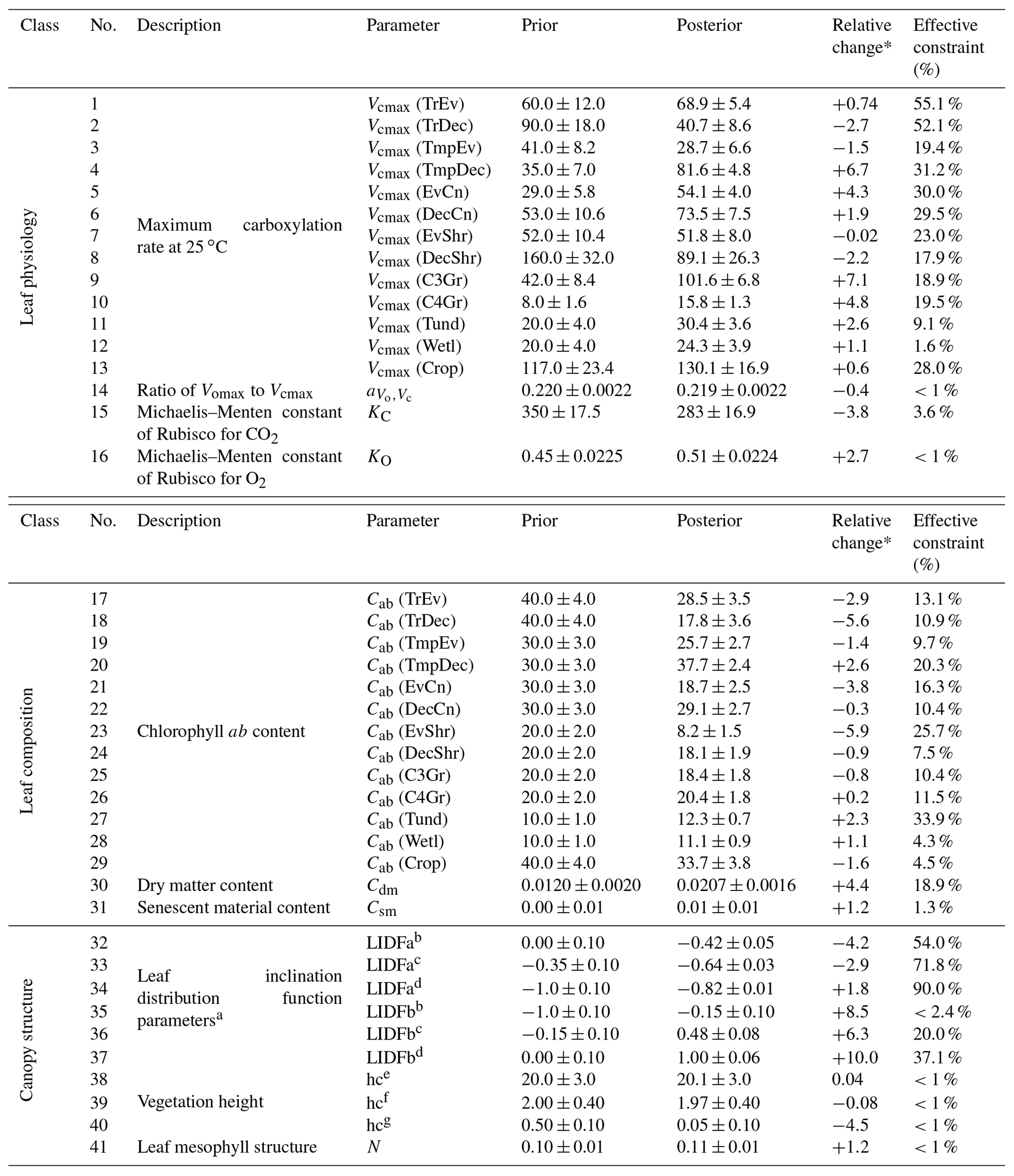
* The relative change is the parameter change in multiples of prior uncertainty. a Prior values based on Verhoef and Bach (2007). b Applies to PFTs TrEv, TrDec, TmpEv, TmpDec, EvShr, DecShr. c Applies to PFTs EvCn, DecCn, Tund. d Applies to PFTs C3Gr, C4Gr, Wetl, Crop. e Applies to PFTs TrEv, TrDec, TmpEv, TmpDec, EvCn, DecCn. f Applies to PFTs. EvShr, DecShr. g Applies to PFTs C3Gr, C4Gr, Tund, Wetl, Crop.
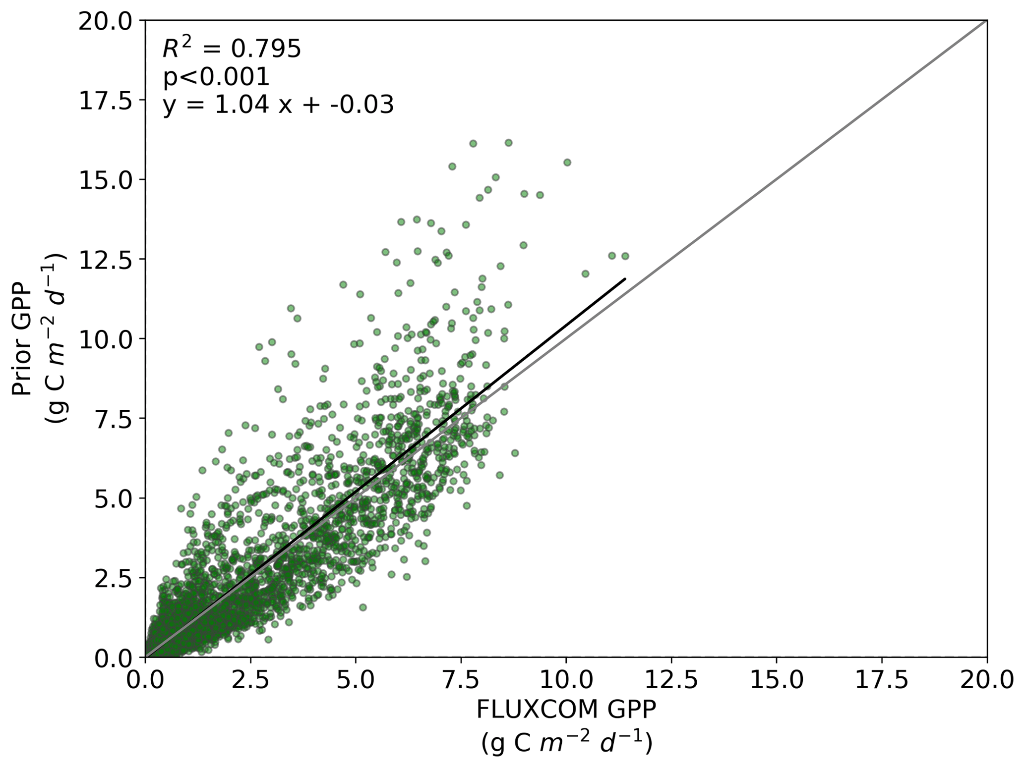
Figure B1Comparison between FLUXCOM GPP and BETHY-SCOPE prior GPP over continental North America (between 24 and 56∘ N).
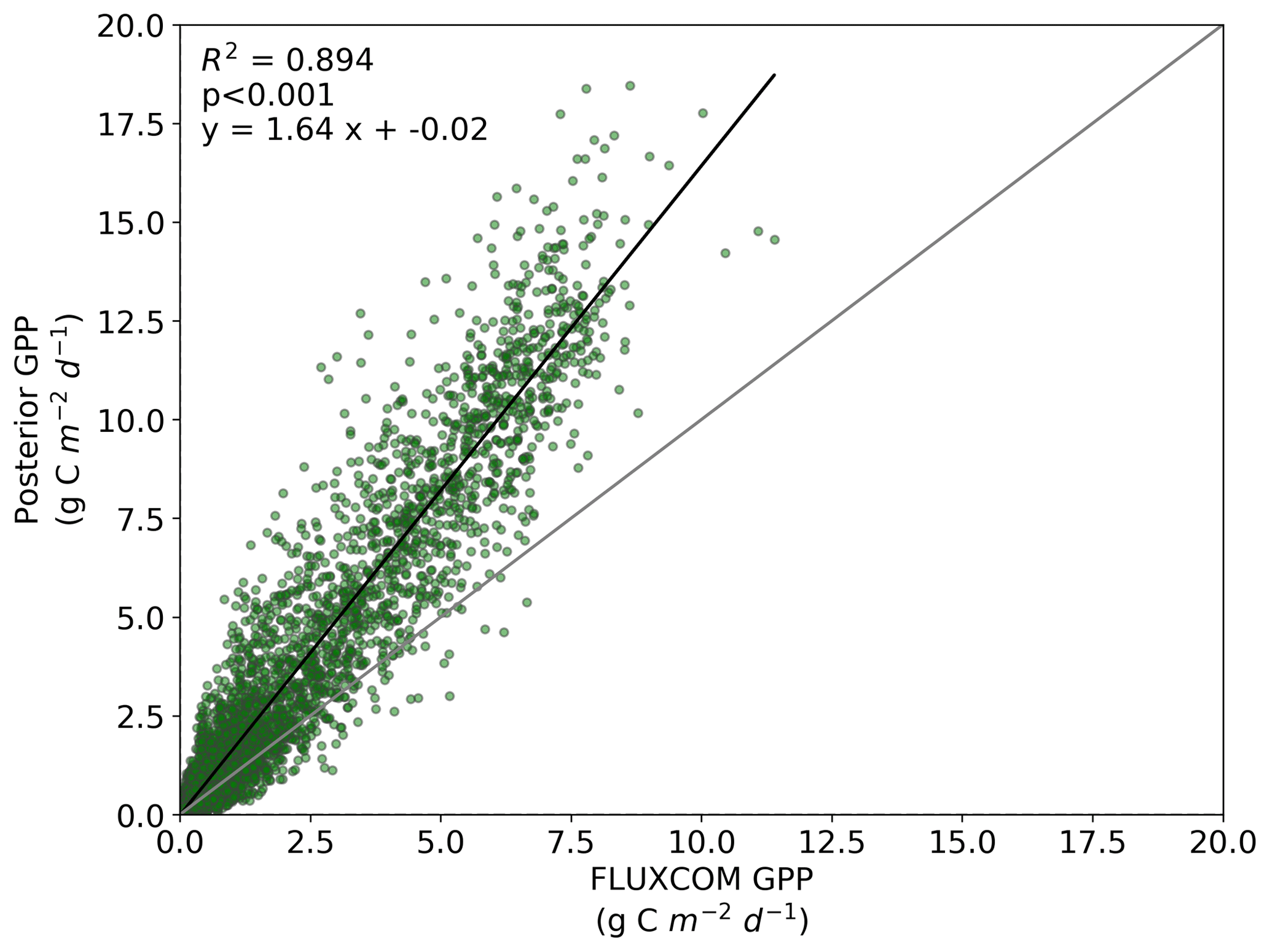
Figure B2Comparison between FLUXCOM GPP and BETHY-SCOPE posterior GPP over continental North America (between 24 and 56∘ N).
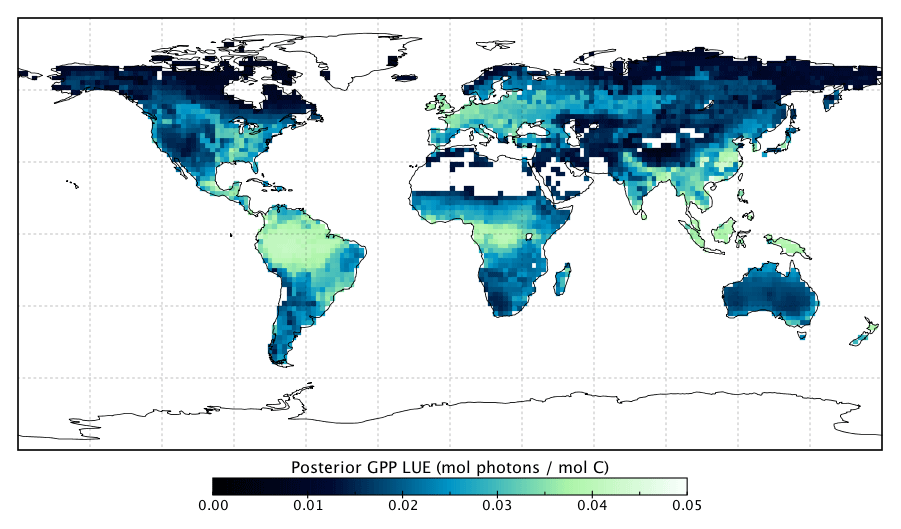
Figure B3Posterior annual mean LUEGPP following the SIF assimilation.
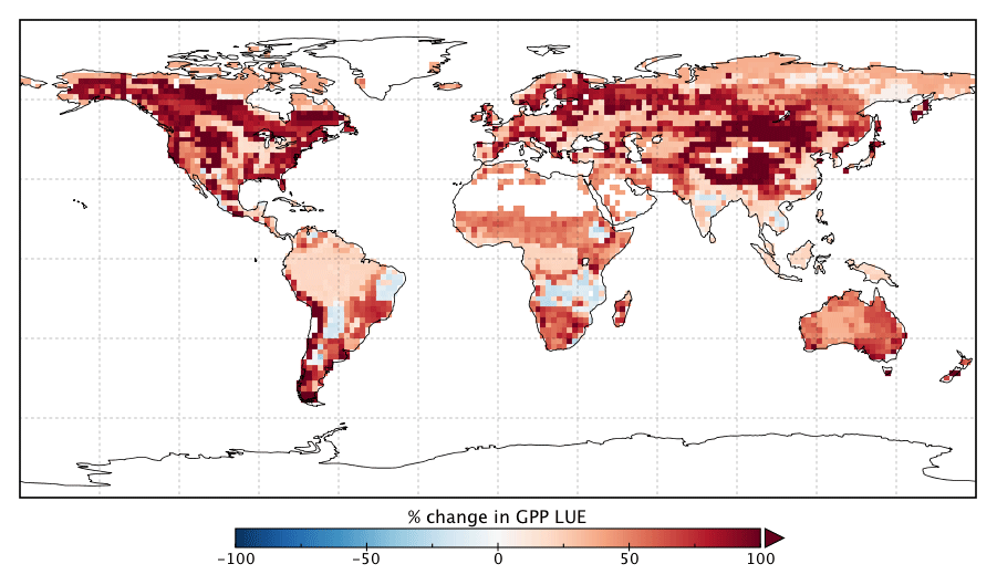
Figure B4Percentage change in annual mean LUEGPP following the SIF assimilation.
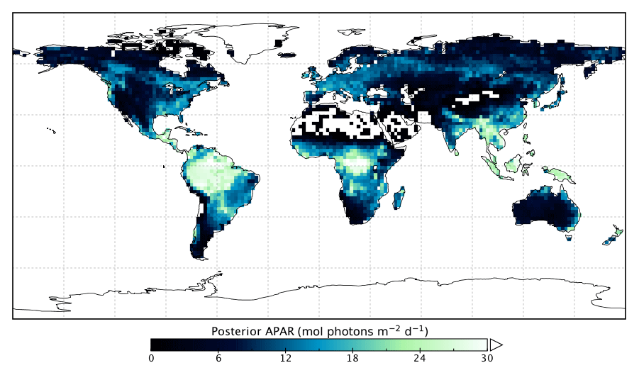
Figure B5Posterior annual mean APAR following the SIF assimilation.

Figure B6Percentage change in annual mean APAR following the SIF assimilation.
Table B1Estimated GPP per biome and latitudinal region, given as GPP rate and total annual GPP (in brackets). Biomes are defined by the spatially dominant PFT as shown in Fig. A1. The tropics are defined as the region between 30∘ S and 30∘ N and the extratropics is defined as all latitudes outside of the tropics. The boreal region is defined as north of 54∘ N. The temperate region is defined as south of 30∘ S and 30–54∘ N.

The supplement related to this article is available online at: https://doi.org/10.5194/bg-16-3069-2019-supplement.
AJN and PJR designed the study and performed the model simulations and data analysis. AJN prepared the manuscript and handled the edits. ENK conducted the initial coupling of the BETHY and SCOPE models. ENK and MS also contributed to further model development and manuscript revisions. JDS contributed to improving the efficiency of model simulations and analysis. YPW contributed to the interpretation of results and manuscript revisions.
The authors declare that they have no conflict of interest.
This research was undertaken with the assistance of resources and services from the National Computational Infrastructure (NCI), which is supported by the Australian Government. We acknowledge the efforts of the TRENDY modeling group and thank them for supplying the TRENDY model data. We acknowledge the efforts of the OCO-2 science team and Christian Frankenberg for his assistance with the satellite SIF data.
Alexander J. Norton was partly supported by an Australian Postgraduate Award from the Australian Government and a CSIRO OCE Scholarship. This research benefited from support provided by the ARC Centre of Excellence for Climate System Science (grant no. CE110001028). Peter J. Rayner was supported by an Australian Research Council Fellowship (grant no. DP1096309).
This paper was edited by Akihiko Ito and reviewed by two anonymous referees.
Ali, A. A., Xu, C., Rogers, A., Mcdowell, N. G., Medlyn, B. E., Fisher, R. A., Wullschleger, S. D., Reich, P. B., Vrugt, J. A., Bauerle, W. L., Santiago, L. S., and Wilson, C. J.: Global-scale environmental control of plant photosynthetic capacity, Ecol. Appl., 25, 2349–2365, 2015. a
Alton, P. B.: Decadal trends in photosynthetic capacity and leaf area index inferred from satellite remote sensing for global vegetation types, Agr. Forest Meteorol., 250-251, 361–375, https://doi.org/10.1016/j.agrformet.2017.11.020, 2018. a
Anav, A., Friedlingstein, P., Beer, C., Ciais, P., Harper, A., Jones, C., Murray-Tortarolo, G., Papale, D., Parazoo, N. C., Peylin, P., Piao, S., Sitch, S., Viovy, N., Wiltshire, A., and Zhao, M.: Spatiotemporal patterns of terrestrial gross primary production: A review, Rev. Geophys., 53, 785–818, https://doi.org/10.1002/2015RG000483, 2015. a, b, c, d
Bacour, C., Peylin, P., Macbean, N., Rayner, P. J., Delage, F., Chevallier, F., Weiss, M., Demarty, J., Santaren, D., Baret, F., Berveiller, D., Dufrêne, E., and Prunet, P.: Joint assimilation of eddy covariance flux measurements and FAPAR products over temperate forests within a process-oriented biosphere model, J. Geophys. Res.-Biogeo., 120, 1839–1857, https://doi.org/10.1002/2015JG002966, 2015. a
Badgley, G., Anderegg, L. D. L., Berry, J. A., and Field, C. B.: An ecologically based approach to terrestrial primary production, EarthArXiv, https://doi.org/10.31223/osf.io/s6t3z, 2018. a
Baker, N. R.: Chlorophyll fluorescence: a probe of photosynthesis in vivo, Annu. Rev. Plant Biol., 59, 89–113, https://doi.org/10.1146/annurev.arplant.59.032607.092759, 2008. a, b
Bayat, B., van der Tol, C., Yang, P., and Verhoef, W.: Extending the SCOPE model to combine optical reflectance and soil moisture observations for remote sensing of ecosystem functioning under water stress conditions, Remote Sens. Environ., 221, 286–301, https://doi.org/10.1016/j.rse.2018.11.021, 2019. a, b
Björkman, O.: Responses to different quantum flux densities, in: Physiological Plant Ecology I: Responses to physical environment, edited by: Lange, O., Nobel, P., Osmond, C., and Ziegler, H., Vol. 12A, 57–107, Springer, Heidelberg, Berlin, and New York, https://doi.org/10.1111/aji.12612, 1981. a, b
Björkman, O. and Demmig, B.: Photon yield of O2 evolution and chlorophyll fluorescence characteristics at 77 K among vascular plants of diverse origins, Planta, 170, 489–504, https://doi.org/10.1007/BF00402983, 1987. a
Campbell, J. E., Carmichael, G. R., Chai, T., Mena-Carrasco, M., Tang, Y., Blake, D. R., Blake, N. J., Vay, S. A., Collatz, G. J., Baker, I., Berry, J. A., Montzka, S. A., Sweeney, C., Schnoor, J. L., and Stanier, C. O.: Photosynthetic control of atmospheric carbonyl sulfide during the growing season, Science, 322, 1085–1088, https://doi.org/10.1126/science.1164015, 2008. a
Campbell, J. E., Berry, J. A., Seibt, U., Smith, S. J., Montzka, S. A., Launois, T., Belviso, S., Bopp, L., and Laine, M.: Large historical growth in global terrestrial gross primary production, Nature, 544, 84–87, https://doi.org/10.1038/nature22030, 2017. a
Collatz, G., Ball, J., Grivet, C., and Berry, J.: Physiological and environmental regulation of stomatal conductance, photosynthesis and transpiration: a model that includes a laminar boundary layer, Agr. Forest Meteorol., 51, 659–668, https://doi.org/10.1016/0168-1923(91)90002-8, 1991. a
Collatz, G., Ribas-Carbo, M., and Berry, J.: Coupled photosynthesis-stomatal conductance model for leaves of C4 plants, Aust. J. Plant Physiol., 19, 519–538, https://doi.org/10.1071/PP9920519, 1992. a
Demarez, V.: Seasonal variation of leaf chlorophyll content of a temperate forest. Inversion of the PROSPECT model, Int. J. Remote Sens., 20, 879–894, https://doi.org/10.1080/014311699212975, 1999. a
Demmig-Adams, B. and Adams III, W. W.: Photoprotection in an ecological context : the remarkable complexity of thermal energy dissipation, New Phytol., 172, 11–21, 2006. a
Duveiller, G. and Cescatti, A.: Spatially downscaling sun-induced chlorophyll fluorescence leads to an improved temporal correlation with gross primary productivity, Remote Sens. Environ., 182, 72–89, https://doi.org/10.1016/j.rse.2016.04.027, 2016. a
Evans, J. R.: Photosynthesis and nitrogen relationships in leaves of C3 plants, Oecologia, 78, 9–19, 1989. a
Farquhar, G. D., von Caemmerer, S., and Berry, J. A.: A biochemical model of photosynthetic CO2 assimilation in leaves of C3 species, Planta, 90, 78–90, 1980. a
Fleming, G. R., Schlau-Cohen, G. S., Amarnath, K., and Zaks, J.: Design principles of photosynthetic light-harvesting, Faraday Discuss., 155, 27, https://doi.org/10.1039/c1fd00078k, 2012. a
Flexas, J., Escalona, J. M., Evain, S., Gulías, J., Moya, I., Osmond, C. B., and Medrano, H.: Steady-state chlorophyll fluorescence (Fs) measurements as a tool to follow variations of net CO2 assimilation and stomatal conductance during water-stress in C3 plants, Physiol. Plantarum, 114, 231–240, 2002. a
Fox, A., Williams, M., Richardson, A. D., Cameron, D., Gove, J. H., Quaife, T., Ricciuto, D., Reichstein, M., Tomelleri, E., Trudinger, C. M., and Wijk, M. T. V.: The REFLEX project: Comparing different algorithms and implementations for the inversion of a terrestrial ecosystem model against eddy covariance data, Agr. Forest Meteorol., 149, 1597–1615, https://doi.org/10.1016/j.agrformet.2009.05.002, 2009. a
Frankenberg, C., Butz, A., and Toon, G. C.: Disentangling chlorophyll fluorescence from atmospheric scattering effects in O2 A-band spectra of reflected sun-light, Geophys. Res. Lett., 38, L03801, https://doi.org/10.1029/2010GL045896, 2011a. a, b
Frankenberg, C., Fisher, J. B., Worden, J., Badgley, G., Saatchi, S. S., Lee, J.-E., Toon, G. C., Butz, A., Jung, M., Kuze, A., and Yokota, T.: New global observations of the terrestrial carbon cycle from GOSAT: Patterns of plant fluorescence with gross primary productivity, Geophys. Res. Lett., 38, L17706, https://doi.org/10.1029/2011GL048738, 2011b. a
Frankenberg, C., O'Dell, C., Berry, J., Guanter, L., Joiner, J., Köhler, P., Pollock, R., and Taylor, T. E.: Prospects for chlorophyll fluorescence remote sensing from the Orbiting Carbon Observatory-2, Remote Sens. Environ., 147, 1–12, https://doi.org/10.1016/j.rse.2014.02.007, 2014. a, b, c, d
Friedl, M., Strahler, A., Hodges, J., Hall, F., Collatz, G., Meeson, B., Los, S., Brown De Colstoun, E., and Landis, D.: ISLSCP II MODIS (Collection 4) IGBP Land Cover, 2000–2001, ORNL DAAC, Oak Ridge, Tennessee, USA, https://doi.org/10.3334/ORNLDAAC/968, 2010. a
Friedlingstein, P., Meinshausen, M., Arora, V. K., Jones, C. D., Anav, A., Liddicoat, S. K., and Knutti, R.: Uncertainties in CMIP5 Climate Projections due to Carbon Cycle Feedbacks, J. Climate, 27, 511–526, https://doi.org/10.1175/JCLI-D-12-00579.1, 2014. a
Gastellu-Etchegorry, J. P., Lauret, N., Yin, T., Landier, L., Kallel, A., Malenovský, Z., Al Bitar, A., Aval, J., Benhmida, S., Qi, J., Medjdoub, G., Guilleux, J., Chavanon, E., Cook, B., Morton, D., Chrysoulakis, N., and Mitraka, Z.: DART: Recent advances in remote sensing data modeling with atmosphere, polarization, and chlorophyll fluorescence, IEEE J. Sel. Top. Appl., 10, 2640–2649, https://doi.org/10.1109/JSTARS.2017.2685528, 2017. a
Genty, B., Briantais, J.-M., and Baker, N. R.: The relationship between the quantum yield of photosynthetic electron transport and quenching of chlorophyll fluorescence, Biochim. Biophys. Acta, 990, 87–92, https://doi.org/10.1016/S0304-4165(89)80016-9, 1989. a, b
Govindjee: Sixty-three years since Kautsky: Chlorophyll a Fluorescence, Aust. J. Plant Physiol., 22, 131–160, 1995. a, b
Guan, K., Berry, J. A., Zhang, Y., Joiner, J., Guanter, L., Badgley, G., and Lobell, D. B.: Improving the monitoring of crop productivity using spaceborne solar-induced fluorescence, Glob. Change Biol., 22, 716–726, https://doi.org/10.1111/gcb.13136, 2015. a
Guanter, L., Frankenberg, C., Dudhia, A., Lewis, P. E., Gómez-Dans, J., Kuze, A., Suto, H., and Grainger, R. G.: Retrieval and global assessment of terrestrial chlorophyll fluorescence from GOSAT space measurements, Remote Sens. Environ., 121, 236–251, https://doi.org/10.1016/j.rse.2012.02.006, 2012. a, b
Guanter, L., Zhang, Y., Jung, M., Joiner, J., Voigt, M., Berry, J. a., Frankenberg, C., Huete, A. R., Zarco-Tejada, P., Lee, J.-E., Moran, M. S., Ponce-Campos, G., Beer, C., Camps-Valls, G., Buchmann, N., Gianelle, D., Klumpp, K., Cescatti, A., Baker, J. M., and Griffis, T. J.: Global and time-resolved monitoring of crop photosynthesis with chlorophyll fluorescence, P. Natl. Acad. Sci. USA, 111, E1327–E1333, https://doi.org/10.1073/pnas.1320008111, 2014. a
Hirose, T. and Werger, M. J. A.: Maximizing daily canopy photosynthesis with respect to the leaf nitrogen allocation pattern in the canopy, Oecologia, 72, 520–526, https://doi.org/10.1007/BF00378977, 1987. a
Jacquemoud, S. and Baret, F.: PROSPECT: A Model of Leaf Optical Properties Spectra, Remote Sens. Environ., 34, 75–91, https://doi.org/10.1016/0034-4257(90)90100-Z, 1990. a
Janssens, I. A., Freibauer, A., Ciais, P., Smith, P., Nabuurs, G.-J., Folberth, G., Schlamadinger, B., Hutjes, R. W. A., Ceulemans, R., Schulze, E. D., Valentini, R., and Dolman, A. J.: Europe's terrestrial biosphere absorbs 7 to 12 % of European anthropogenic CO2 emissions, Science, 300, 1538–1542, https://doi.org/10.1126/science.1083592, 2003. a
Joiner, J., Yoshida, Y., Vasilkov, A. P., Yoshida, Y., Corp, L. A., and Middleton, E. M.: First observations of global and seasonal terrestrial chlorophyll fluorescence from space, Biogeosciences, 8, 637–651, https://doi.org/10.5194/bg-8-637-2011, 2011. a, b, c
Joiner, J., Yoshida, Y., Vasilkov, A. P., Schaefer, K., Jung, M., Guanter, L., Zhang, Y., Garrity, S., Middleton, E. M., Huemmrich, K. F., Gu, L., and Marchesini, L. B.: The seasonal cycle of satellite chlorophyll fluorescence observations and its relationship to vegetation phenology and ecosystem atmosphere carbon exchange, Remote Sens. Environ., 152, 375–391, https://doi.org/10.1016/j.rse.2014.06.022, 2014. a, b
Jung, M., Reichstein, M., Margolis, H. A., Cescatti, A., Richardson, A. D., Arain, M. A., Arneth, A., Bernhofer, C., Bonal, D., Chen, J., Gianelle, D., Gobron, N., Kiely, G., Kutsch, W., Lasslop, G., Law, B. E., Lindroth, A., Merbold, L., Montagnani, L., Moors, E. J., Papale, D., Sottocornola, M., Vaccari, F., and Williams, C.: Global patterns of land-atmosphere fluxes of carbon dioxide, latent heat, and sensible heat derived from eddy covariance, satellite, and meteorological observations, J. Geophys. Res.-Biogeo., 116, 1–16, https://doi.org/10.1029/2010JG001566, 2011. a
Kaminski, T., Knorr, W., Scholze, M., Gobron, N., Pinty, B., Giering, R., and Mathieu, P.-P.: Consistent assimilation of MERIS FAPAR and atmospheric CO2 into a terrestrial vegetation model and interactive mission benefit analysis, Biogeosciences, 9, 3173–3184, https://doi.org/10.5194/bg-9-3173-2012, 2012. a, b
Kaminski, T., Knorr, W., Schürmann, G., Scholze, M., Rayner, P. J., Zaehle, S., Blessing, S., Dorigo, W., Gayler, V., Giering, R., Gobron, N., Grant, J. P., Heimann, M., Houweling, S., Kato, T., Kattge, J., Kelley, D., Kemp, S., Koffi, E. N., Köstler, C., Mathieu, P., Pinty, B., Reick, C. H., Rödenbeck, C., Schnur, R., Scipal, K., Sebald, C., Stacke, T., Van, A. T., Vossbeck, M., Widmann, H., and Ziehn, T.: The BETHY/JSBACH Carbon Cycle Data Assimilation System: experiences and challenges, J. Geophys. Res.-Biogeo., 118, 1–13, https://doi.org/10.1002/jgrg.20118, 2013. a, b, c, d
Kato, T., Knorr, W., Scholze, M., Veenendaal, E., Kaminski, T., Kattge, J., and Gobron, N.: Simultaneous assimilation of satellite and eddy covariance data for improving terrestrial water and carbon simulations at a semi-arid woodland site in Botswana, Biogeosciences, 10, 789–802, https://doi.org/10.5194/bg-10-789-2013, 2013. a
Knorr, W.: Annual and interannual CO2 exchanges of the terrestrial biosphere: process-based simulations and uncertainties, Global Ecol. Biogeogr., 9, 225–252, https://doi.org/10.1046/j.1365-2699.2000.00159.x, 2000. a
Knorr, W., Kaminski, T., Scholze, M., Gobron, N., Pinty, B., Giering, R., and Mathieu, P.-P.: Carbon cycle data assimilation with a generic phenology model, J. Geophys. Res., 115, G04017, https://doi.org/10.1029/2009JG001119, 2010. a, b, c
Koffi, E. N., Rayner, P. J., Scholze, M., and Beer, C.: Atmospheric constraints on gross primary productivity and net ecosystem productivity: Results from a carbon-cycle data assimilation system, Global Biogeochem. Cy., 26, 1–16, https://doi.org/10.1029/2010GB003900, 2012. a, b
Koffi, E. N., Rayner, P. J., Norton, A. J., Frankenberg, C., and Scholze, M.: Investigating the usefulness of satellite-derived fluorescence data in inferring gross primary productivity within the carbon cycle data assimilation system, Biogeosciences, 12, 4067–4084, https://doi.org/10.5194/bg-12-4067-2015, 2015. a, b, c, d, e
Köhler, P., Frankenberg, C., Magney, T. S., Guanter, L., Joiner, J., and Landgraf, J.: Global Retrievals of Solar-Induced Chlorophyll Fluorescence With TROPOMI: First Results and Intersensor Comparison to OCO-2, Geophys. Res. Lett., 45, 10456–10463, https://doi.org/10.1029/2018GL079031, 2018. a
Krall, J. and Edwards, G.: Relationship between photosystem II activity and CO2 fixation in leaves, Physiol. Plantarum, 86, 180–187, https://doi.org/10.1111/j.1399-3054.1992.tb01328.x, 1992. a
Kuppel, S., Chevallier, F., and Peylin, P.: Quantifying the model structural error in carbon cycle data assimilation systems, Geosci. Model Dev., 6, 45–55, https://doi.org/10.5194/gmd-6-45-2013, 2013. a, b
Li, X., Xiao, J., He, B., Altaf Arain, M., Beringer, J., Desai, A. R., Emmel, C., Hollinger, D. Y., Krasnova, A., Mammarella, I., Noe, S. M., Ortiz, P. S., Rey-Sanchez, A. C., Rocha, A. V., and Varlagin, A.: Solar-induced chlorophyll fluorescence is strongly correlated with terrestrial photosynthesis for a wide variety of biomes: First global analysis based on OCO-2 and flux tower observations, Glob. Change Biol., 24, 3990–4008, https://doi.org/10.1111/gcb.14297, 2018. a, b
Luus, K. A., Commane, R., Parazoo, N. C., Benmergui, J., Euskirchen, E. S., Frankenberg, C., Joiner, J., Lindass, J., Miller, C. E., Oechel, W. C., Zona, D., Wofsy, S., and Lin, J. C.: Tundra photosynthesis captured by satellite-observed solar-induced chlorophyll fluorescence, Geophys. Res. Lett., 44, 1564–1573, https://doi.org/10.1002/2016GL070842, 2017. a, b
MacBean, N., Peylin, P., Chevallier, F., Scholze, M., and Schürmann, G.: Consistent assimilation of multiple data streams in a carbon cycle data assimilation system, Geosci. Model Dev., 9, 3569–3588, https://doi.org/10.5194/gmd-9-3569-2016, 2016. a, b
MacBean, N., Maignan, F., Bacour, C., Lewis, P., Peylin, P., Guanter, L., Köhler, P., Gómez-Dans, J., and Disney, M.: Strong constraint on modelled global carbon uptake using solar-induced chlorophyll fluorescence data, Sci. Rep.-UK, 8, 1–12, https://doi.org/10.1038/s41598-018-20024-w, 2018. a, b, c, d, e, f, g, h
Miller, J., Berger, M., Goulas, Y., Jacquemoud, S., Louis, J., Mohammed, G., Moise, N., Moreno, J., Moya, I., and Pedrós, R.: Development of a vegetation fluorescence canopy model, Tech. rep., ESA Scientific and Technical Publications Branch, ESTEC, available at: http://quantalab.ias.csic.es/fluormod/ (last access: 4 August 2019) 2005. a
Norton, A. J., Rayner, P. J., Koffi, E. N., and Scholze, M.: Assimilating solar-induced chlorophyll fluorescence into the terrestrial biosphere model BETHY-SCOPE v1.0: model description and information content, Geosci. Model Dev., 11, 1517–1536, https://doi.org/10.5194/gmd-11-1517-2018, 2018. a, b, c, d, e, f, g, h, i, j, k, l, m, n, o
Parazoo, N. C., Bowman, K., Fisher, J. B., Frankenberg, C., Jones, D. B. A., Cescatti, A., Perez-Priego, O., Wohlfahrt, G., and Montagnani, L.: Terrestrial gross primary production inferred from satellite fluorescence and vegetation models, Glob. Change Biol., 20, 3103–3121, https://doi.org/10.1111/gcb.12652, 2014. a, b, c, d, e
Peylin, P., Bacour, C., MacBean, N., Leonard, S., Rayner, P., Kuppel, S., Koffi, E., Kane, A., Maignan, F., Chevallier, F., Ciais, P., and Prunet, P.: A new stepwise carbon cycle data assimilation system using multiple data streams to constrain the simulated land surface carbon cycle, Geosci. Model Dev., 9, 3321–3346, https://doi.org/10.5194/gmd-9-3321-2016, 2016. a, b
Porcar-Castell, A., Tyystjärvi, E., Atherton, J., van der Tol, C., Flexas, J., Pfündel, E. E., Moreno, J., Frankenberg, C., and Berry, J. A.: Linking chlorophyll a fluorescence to photosynthesis for remote sensing applications: mechanisms and challenges, J. Exp. Botany, 65, 4065–95, https://doi.org/10.1093/jxb/eru191, 2014. a, b, c
Raczka, B., Porcar‐Castell, A., Magney, T., Lee, J., Köhler, P., Frankenberg, C., Grossmann, K., Logan, B., Stutz, J., Blanken, P., Burns, S., Duarte, H., Yang, X., Lin, J., and Bowling, D.: Sustained Non‐Photochemical Quenching Shapes the Seasonal Pattern of Solar‐ Induced Fluorescence at a High‐Elevation Evergreen Forest, J. Geophys. Res.-Biogeo., https://doi.org/10.1029/2018JG004883, online first, 2019. a
Rayner, P., Scholze, M., Knorr, W., and Kaminski, T.: Two decades of terrestrial carbon fluxes from a carbon cycle data assimilation system (CCDAS), Global Biogeochem. Cy., 19, GB2026, https://doi.org/10.1029/2004GB002254, 2005. a, b, c, d
Rayner, P. J.: The current state of carbon-cycle data assimilation, Curr. Opin. Env. Sust., 2, 289–296, https://doi.org/10.1016/j.cosust.2010.05.005, 2010. a
Schimel, D., Pavlick, R., Fisher, J. B., Asner, G. P., Saatchi, S., Townsend, P., Miller, C., Frankenberg, C., Hibbard, K., and Cox, P.: Observing terrestrial ecosystems and the carbon cycle from space, Glob. Change Biol., 21, 1762–1776, https://doi.org/10.1111/gcb.12822, 2015. a
Scholze, M., Kaminski, T., Rayner, P., Knorr, W., and Giering, R.: Propagating uncertainty through prognostic carbon cycle data assimilation system simulations, J. Geophys. Res., 112, D17305, https://doi.org/10.1029/2007JD008642, 2007. a, b
Scholze, M., Kaminski, T., Knorr, W., Blessing, S., Vossbeck, M., Grant, J. P., and Scipal, K.: Simultaneous assimilation of SMOS soil moisture and atmospheric CO2 in-situ observations to constrain the global terrestrial carbon cycle, Remote Sens. Environ., 180, 334–345, https://doi.org/10.1016/j.rse.2016.02.058, 2016. a, b
Sitch, S., Friedlingstein, P., Gruber, N., Jones, S. D., Murray-Tortarolo, G., Ahlström, A., Doney, S. C., Graven, H., Heinze, C., Huntingford, C., Levis, S., Levy, P. E., Lomas, M., Poulter, B., Viovy, N., Zaehle, S., Zeng, N., Arneth, A., Bonan, G., Bopp, L., Canadell, J. G., Chevallier, F., Ciais, P., Ellis, R., Gloor, M., Peylin, P., Piao, S. L., Le Quéré, C., Smith, B., Zhu, Z., and Myneni, R.: Recent trends and drivers of regional sources and sinks of carbon dioxide, Biogeosciences, 12, 653–679, https://doi.org/10.5194/bg-12-653-2015, 2015. a, b
Sun, Y., Frankenberg, C., Jung, M., Joiner, J., Guanter, L., Köhler, P., and Magney, T.: Overview of Solar-Induced chlorophyll Fluorescence (SIF) from the Orbiting Carbon Observatory-2: Retrieval, cross-mission comparison, and global monitoring for GPP, Remote Sens. Environ., 209, 808–823, https://doi.org/10.1016/j.rse.2018.02.016, 2018. a, b, c, d, e, f, g
Tarantola, A.: Inverse Problem Theory: Methods for Data Fitting and Model Parameter Estimation, 1st Edn., Elsevier, New York, 1987. a
Tarantola, A.: Inverse Problem Theory and Methods for Model Parameter Estimation, SIAM, Philadelphia, 2005. a, b, c, d
Tramontana, G., Jung, M., Schwalm, C. R., Ichii, K., Camps-Valls, G., Ráduly, B., Reichstein, M., Arain, M. A., Cescatti, A., Kiely, G., Merbold, L., Serrano-Ortiz, P., Sickert, S., Wolf, S., and Papale, D.: Predicting carbon dioxide and energy fluxes across global FLUXNET sites with regression algorithms, Biogeosciences, 13, 4291–4313, https://doi.org/10.5194/bg-13-4291-2016, 2016. a, b, c, d
Trudinger, C. M., Raupach, M. R., Rayner, P. J., Kattge, J., Liu, Q., Pak, B., Reichstein, M., Renzullo, L., Richardson, A. D., Roxburgh, S. H., Styles, J., Wang, Y. P., Briggs, P., Barrett, D., and Nikolova, S.: OptIC project: An intercomparison of optimization techniques for parameter estimation in terrestrial biogeochemical models, J. Geophys. Res., 112, G02027, https://doi.org/10.1029/2006JG000367, 2007. a
van der Tol, C., Verhoef, W., Timmermans, J., Verhoef, A., and Su, Z.: An integrated model of soil-canopy spectral radiances, photosynthesis, fluorescence, temperature and energy balance, Biogeosciences, 6, 3109–3129, https://doi.org/10.5194/bg-6-3109-2009, 2009. a, b, c, d
van der Tol, C., Berry, J. A., Campbell, P. K. E., and Rascher, U.: Models of fluorescence and photosynthesis for interpreting measurements of solar-induced chlorophyll fluorescence, J. Geophys. Res.-Biogeo., 119, 1–16, https://doi.org/10.1002/2014JG002713, 2014. a, b, c, d, e, f, g, h
Verhoef, W.: Light scattering by leaf layers with application to canopy reflectance modeling: The SAIL model, Remote Sens. Environ., 16, 125–141, https://doi.org/10.1016/0034-4257(84)90057-9, 1984. a
Verhoef, W. and Bach, H.: Coupled soil–leaf-canopy and atmosphere radiative transfer modeling to simulate hyperspectral multi-angular surface reflectance and TOA radiance data, Remote Sens. Environ., 109, 166–182, https://doi.org/10.1016/j.rse.2006.12.013, 2007. a
Verrelst, J., Rivera, J. P., Tol, C. V. D., Magnani, F., Mohammed, G., and Moreno, J.: Global sensitivity analysis of the SCOPE model: What drives simulated canopy-leaving sun-induced fluorescence?, Remote Sens. Environ., 166, 8–21, https://doi.org/10.1016/j.rse.2015.06.002, 2015. a
von Caemmerer, S.: Biochemical Models of Photosynthesis, CSIRO Publishing, Collingwood, Australia, 2000. a, b
Walker, A. P., Quaife, T., van Bodegom, P. M., De Kauwe, M. G., Keenan, T. F., Joiner, J., Lomas, M. R., MacBean, N., Xu, C., Yang, X., and Woodward, F. I.: The impact of alternative trait-scaling hypotheses for the maximum photosynthetic carboxylation rate (Vcmax) on global gross primary production, New Phytol., 215, 1370–1386, https://doi.org/10.1111/nph.14623, 2017. a
Walther, S., Voigt, M., Thum, T., Gonsamo, A., Zhang, Y., Koehler, P., Jung, M., Varlagin, A., and Guanter, L.: Satellite chlorophyll fluorescence measurements reveal large-scale decoupling of photosynthesis and greenness dynamics in boreal evergreen forests, Glob. Change Biol., 22, 2979–2996, https://doi.org/10.1111/gcb.13200, 2016. a
Wang, Y. P., Baldocchi, D., Leunig, R., Falge, E., and Vesala, T.: Estimating parameters in a land-surface model by applying nonlinear inversion to eddy covariance flux measurements from eight FLUXNET sites, Glob. Change Biol., 13, 652–670, https://doi.org/10.1111/j.1365-2486.2006.01225.x, 2007. a
Waring, R., Landsberg, J., and Linder, S.: Tamm Review: Insights gained from light use and leaf growth efficiency indices, Forest Ecol. Manage., 379, 232–242, https://doi.org/10.1016/j.foreco.2016.08.023, 2016. a, b
Weedon, G. P., Balsamo, G., Bellouin, N., Gomes, S., Best, M. J., and Viterbo, P.: The WFDEI meteorological forcing data set: WATCH Forcing Data methodology applied to ERA-Interim reanalysis data, Water Resour. Res., 50, 7505–7514, https://doi.org/10.1002/2014WR015638, 2014. a
Welp, L. R., Keeling, R. F., Meijer, H. A. J., Bollenbacher, A. F., Piper, S. C., Yoshimura, K., Francey, R. J., Allison, C. E., and Wahlen, M.: Interannual variability in the oxygen isotopes of atmospheric CO2 driven by El Nino, Nature, 477, 579–582, https://doi.org/10.1038/nature10421, 2011. a
Wilson, K. B., Baldocchi, D. D., and Hanson, P. J.: Spatial and seasonal variability of photosynthetic parameters and their relationship to leaf nitrogen in a deciduous forest, Tree Physiol., 20, 565–578, https://doi.org/10.1093/treephys/20.9.565, 2000. a
Wilson, M. and Henderson-Sellers, A.: Global archive of land cover and soils data for use in general-circulation climate models, Int. J. Climatol., 5, 119–143, 1985. a
Xu, L. and Baldocchi, D. D.: Seasonal trends in photosynthetic parameters and stomatal conductance of blue oak (Quercus douglasii) under prolonged summer drought and high temperature, Tree Physiol., 23, 865–877, 2003. a
Yang, K., Ryu, Y., Dechant, B., Berry, J. A., Hwang, Y., Jiang, C., Kang, M., Kim, J., Kimm, H., Kornfeld, A., and Yang, X.: Sun-induced chlorophyll fluorescence is more strongly related to absorbed light than to photosynthesis at half-hourly resolution in a rice paddy, Remote Sens. Environ., 216, 658–673, https://doi.org/10.1016/j.rse.2018.07.008, 2018. a
Yang, X., Tang, J., Mustard, J. F., Lee, J.-E., Rossini, M., Joiner, J., Munger, J. W., Kornfeld, A., and Richardson, A. D.: Solar-induced chlorophyll fluorescence that correlates with canopy photosynthesis on diurnal and seasonal scales in a temperate deciduous forest, Geophys. Res. Lett., 42, 2977–2987, https://doi.org/10.1002/2015GL063201, 2015. a
Yuan, H., Dai, Y., Xiao, Z., Ji, D., and Shangguan, W.: Reprocessing the MODIS Leaf Area Index products for land surface and climate modelling, Remote Sens. Environ., 115, 1171–1187, https://doi.org/10.1016/j.rse.2011.01.001, 2011. a
Zaks, J., Amarnath, K., Sylak-Glassman, E. J., and Fleming, G. R.: Models and measurements of energy-dependent quenching, Photosynth. Res., 116, 389–409, https://doi.org/10.1007/s11120-013-9857-7, 2013. a
Zhang, Y., Guanter, L., Berry, J. A., Joiner, J., van der Tol, C., Huete, A., and Gitelson, A.: Estimation of vegetation photosynthetic capacity from space-based measurements of chlorophyll fluorescence for terrestrial biosphere models, Glob. Change Biol., 20, 3727–3742, https://doi.org/10.1111/gcb.12664, 2014. a
Zhang, Y., Joiner, J., Gentine, P., and Zhou, S.: Reduced solar-induced chlorophyll fluorescence from GOME-2 during Amazon drought caused by dataset artifacts, Glob. Change Biol., 24, 2229–2230, https://doi.org/10.1111/gcb.14134, 2018. a
- Abstract
- Introduction
- Methods
- Results
- Discussion
- Conclusions
- Code and data availability
- Appendix A: Spatially dominant PFT in BETHY-SCOPE model
- Appendix B: Posterior GPP, LUEGPP and APAR patterns
- Author contributions
- Competing interests
- Acknowledgements
- Financial support
- Review statement
- References
- Supplement