2.1 Mesocosm deployment and maintenance

On 22 February 2017, eight Kiel Off-Shore Mesocosms for Future Ocean Simulations (KOSMOS, M1–M8; Riebesell et al., 2013) were deployed with Buque Armada Peruana Morales (BAP Morales) in the SE Pacific, 6 km off the Peruvian coastline (12.0555^∘ S, 77.2348^∘ W; Fig. 1). The water depth at the deployment site was ∼30 m, and the area was protected from southern and southwestern swells by San Lorenzo Island (Fig. 1). The mesocosms consisted of cylindrical, 18.7 m long polyurethane bags (2 m diameter, 54.4±1.3 m³ volume; Table 1) suspended in 8 m tall flotation frames (Fig. 1). The bags were initially folded so that the flotation frames and bags could be lifted with the crane from BAP Morales into the water where the mesocosms were moored with anchor weights. The bags were unfolded immediately after deployment with the lower end extending to ∼19.7 m and the upper end 1 m below the surface. Nets (mesh size 3 mm) attached to both ends of the bags allowed water exchange but prevented larger plankton or nekton from entering the mesocosms. On 25 February, the mesocosms were sealed when divers replaced lower meshes with sediment traps, while upper ends of the bags were pulled ∼1.5 m above the sea surface immediately after sediment trap attachment. These two steps isolated the water mass enclosed inside the mesocosms from the surrounding Pacific water and marked the beginning of the experiment (Day 0; Fig. 2). After the closure, the enclosed water columns were ∼19 m deep of which the lowest 2 m were the conical sediment traps (Fig. 1).

Figure 1The mesocosm study site. (a) Graphic of one KOSMOS unit with underwater bag dimensions given on the left. We acknowledge reprint permission from the AGU as parts of this drawing was used for a publication by Bach et al. (2016b). (b) Overview map of the study region. Please note that the square marking the study site is not true to scale. (c) Detailed map of the study site. The laboratories for sample processing were located in La Punta (Callao). The study site was located at the northern end of San Lorenzo Island. The mesocosm arrangement is shown in the additional square. The stars mark the locations of stations 1 and 3, where the two different OMZ water masses were collected. Coordinates of relevant sites are given in Sect. 2.1.

Table 1Nutrient concentrations at the beginning of the experiment and after the OMZ water addition as well as the mesocosm volumes at the end of the experiment. The color code identifies the “low N∕P” treatment (blue) and the “very low N∕P” treatment (red). $({\mathrm{N}:\mathrm{P}}_{\mathrm{inorg}}=({\mathrm{NO}}_x^{-}+{\mathrm{NH}}_{\mathrm{4}}^{+})/{\mathrm{PO}}_{\mathrm{4}}^{\mathrm{3}-})$. The asterisks indicate significantly different (p<0.05) conditions between the treatments as was calculated with a two-tailed t test after equal variance was confirmed with an F test.

Download Print Version

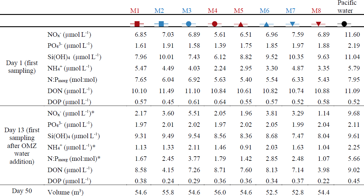
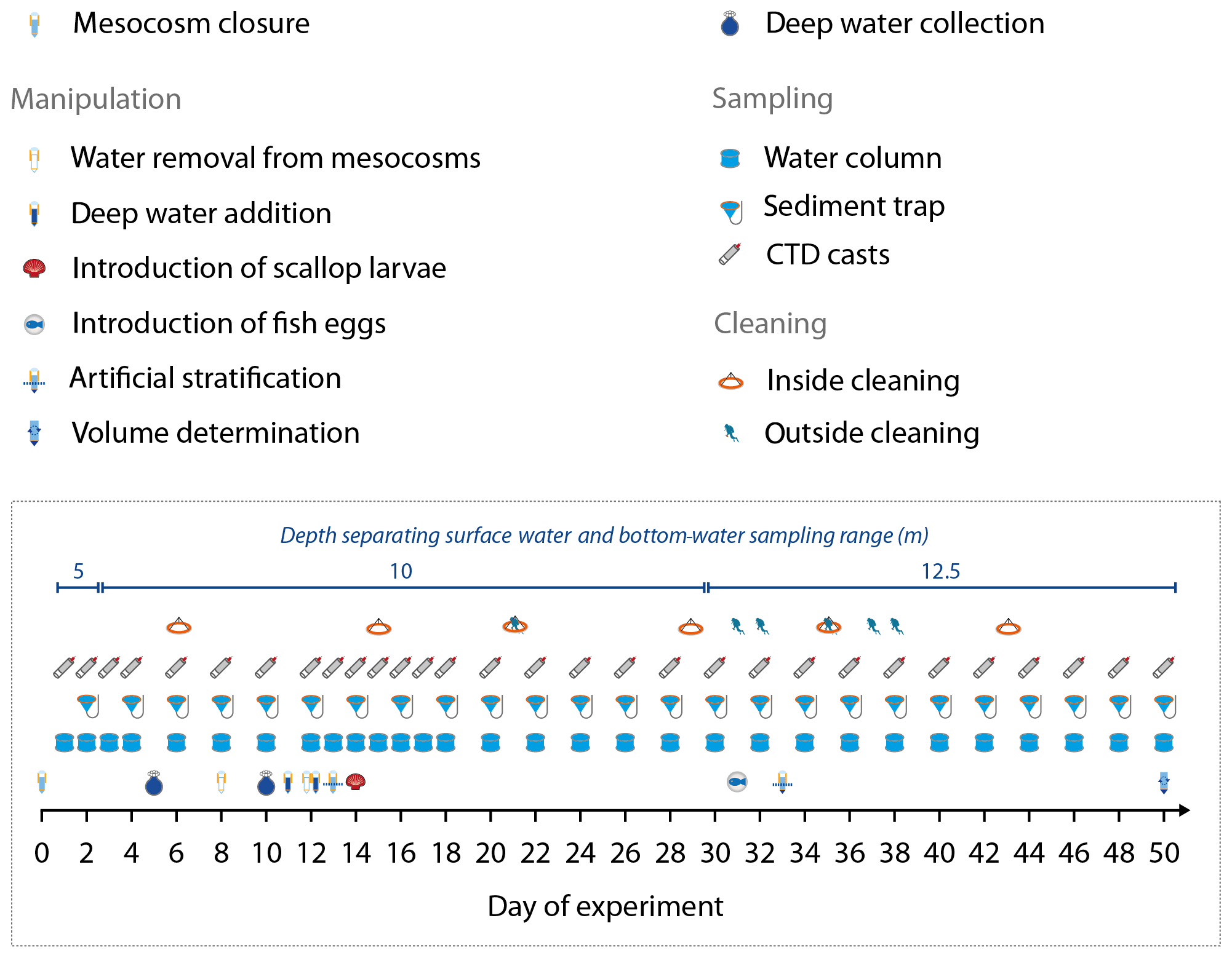
Figure 2Manipulation, sampling, and maintenance schedule. Day 0 was 25 February 2017, and Day 50 was 16 April 2017. Also given is the depth separating the surface water and bottom-water sampling range of the course of the study.

Download

The mesocosm bags were regularly cleaned from the inside and on the outside to minimize biofouling (Fig. 2). Cleaning the outside of the bags was carried out with brushes, either from small boats (0–1.5 m) or by divers (1.5–8 m). The inner sides of the bags were cleaned with rubber blades attached to a polyethylene ring which had the same diameter as the mesocosm bags and was ballasted with a 30 kg weight (Riebesell et al., 2013). The rubber blades were pushed against the walls by the ring and scraped off the organic material while sliding downwards. Cleaning inside down to ∼1 m above the sediment traps was conducted approximately every eighth day to prevent biofouling at an early stage of its progression.

2.2 OMZ water addition to the mesocosms

On 2 and 7 March 2017 (days 5 and 10), we collected two batches of OMZ water (100 m³ each) with Research Vessel IMARPE VI at two different stations of the Instituto del Mar del Perú (IMARPE) time-series transect (Graco et al., 2017). The first batch was collected on Day 5 at station 1 (12.028323^∘ S, 77.223603^∘ W) at a depth of 30 m. The second was collected on Day 10 at station 3 (12.044333^∘ S, 77.377583^∘ W) at a depth of ∼70 m (Fig. 1). In both cases we used deep water collectors described by Taucher et al. (2017). The pear-shaped 100 m³ bags of the collector systems consisted of flexible, fiber-reinforced, food-grade, polyvinyl chloride material (opaque). The round openings of the bags (0.25 m diameter covered with a 10 mm mesh) were equipped with a custom-made propeller system that pumped water into the bag and a shutter system that closed the bag when full. Prior to their deployment, the bags were ballasted with a 300 kg weight so that the bag sank to the desired depth. A rope attached to the bag guaranteed that it did not sink deeper. The propeller and the shutter system were time-controlled and started to fill the bag after it had reached the desired depth and closed the bag after ∼1.5 h of pumping. To recover the collector, the weight was released with an acoustic trigger so that 24 small floats attached to the top made the system positively buoyant and brought it back to the surface. The collectors were towed back to the mesocosm area and moored therein with anchor weights.

On 8 and 9 March 2017 (Day 11 and 12), we exchanged ∼20 m³ of water enclosed in each mesocosm with water collected from station 3 (M2, M3, M6, M7) or station 1 (M1, M4, M5, M8). The exchange was carried out in two steps using a submersible pump (Grundfos SP 17-5R, pump rate ∼18 m³ h⁻¹). On Day 8, we installed the pump for about 30–40 min in each mesocosm and pumped 9 m³ out of each bag from a depth of 11 to 12 m. On Day 11, the pump was installed inside the collector bags, and 10 m³ of water was injected to a 14–17 m depth (hose diameter 5 cm). Please note that the pump (for water withdrawal) and hose (for water injection) were carefully moved up and down the water column between 14 and 17 m so that the water was evenly withdrawn from, or injected into, this depth range. On Day 12, we repeated this entire procedure but this time removed 10 m³ from 8 to 9 m and added 12 m³ evenly to the depth range from 1 to 9 m.

2.3 Salt additions to control stratification and to determine mesocosm volumes

Oxygen minimum zones are a significant feature of EBUS and play an important role for ecological and biogeochemical processes in the Humboldt system (Breitburg et al., 2018; Thiel et al., 2007). They reach very close to the surface (<10 m) in the near-coast region of Peru (Graco et al., 2017); therefore the mesocosms naturally contained water with low O₂ concentrations below ∼10 m (see “Results”). Conserving this oxygen-depleted bottom layer within the mesocosms required artificial water column stratification because heat exchange with the surrounding Pacific water would have destroyed this feature (see Bach et al., 2016a, for a description of the convective-mixing phenomenon in mesocosms). Therefore, we injected 69 L of a concentrated NaCl brine solution evenly into the bottom layers of the mesocosms on Day 13 by carefully moving a custom-made distribution device (Riebesell et al., 2013) up and down between 10 and 17 m. The procedure was repeated on Day 33 with 46 L NaCl brine solution added between 12.5 and 17 m after turbulent mixing between days 13 and 33 continuously blurred the artificial halocline. The brine additions increased bottom-water salinity by about 1 during both additions (Fig. 3b).

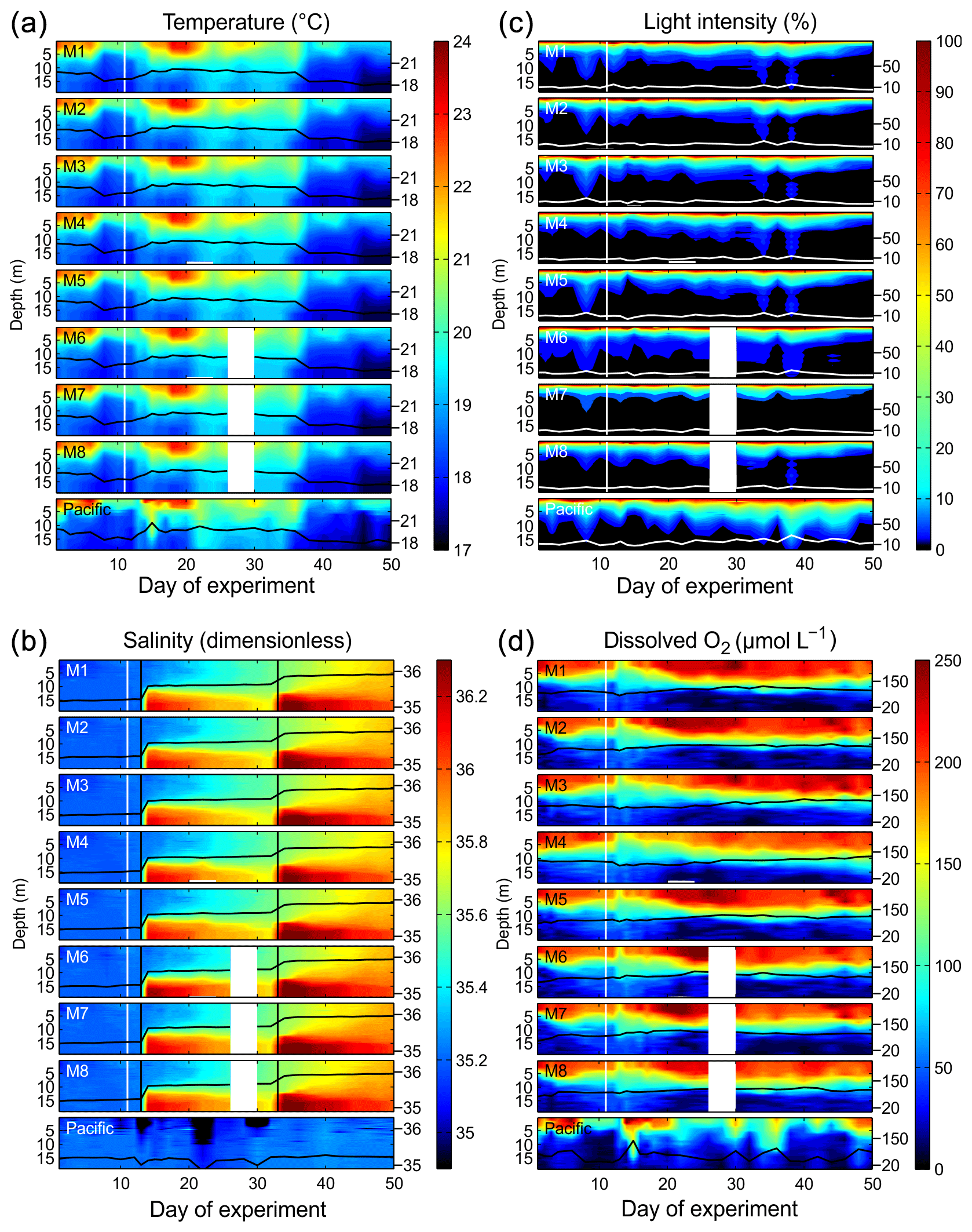
Figure 3Physical and chemical conditions in the enclosed water columns of mesocosms M1–M8 and the Pacific water at the mesocosm mooring site determined with CTD casts. The black (a, b, d) or white (c) lines on top of the contours show the depth-integrated water column average with the corresponding additional y axes on the right side. The vertical white lines indicate the time of OMZ water additions to the mesocosms. The lack of data on Day 28 in M6, M7, and M8 was due to problems with power supply. (a) Temperature in degrees Celsius. (b) Salinity (dimensionless). The vertical black lines mark the NaCl brine additions. (c) Light intensity (photosynthetic active radiation) normalized to surface irradiance in the upper 0.3 m. (d) Dissolved-O₂ concentrations.

Download

At the end of the experiment (Day 50, after the last sampling), we performed a third NaCl brine addition to determine the volume of each mesocosm. For volume determination, we first homogenized the enclosed water columns by pumping compressed air into the bottom layer for 5 min, thereby fully mixing the water masses. This was validated by salinity profiling with subsequent CTD casts (see Sect. 2.4 for CTD specifications). Next, we added 52 kg of a NaCl brine evenly to the entire water column as described above, followed by a second airlift mixing and second set of CTD casts. Since we precisely knew the added amount of NaCl, we were able to determine the volume of the mesocosms at Day 50 from the measured salinity increase as described by Czerny et al. (2013). The mesocosm volumes before Day 50 were calculated for each sampling day based on the volume that was withdrawn during sampling (Sect. 2.5) and exchanged during the OMZ water addition (Sect. 2.2). Rainfall did not occur during the study, and evaporation was negligible (∼1 L d⁻¹) as determined by monitoring salinity over time (Sect. 2.5). These two factors were therefore not considered for the volume calculations.

The NaCl solution used to establish haloclines was prepared in Germany by dissolving 300 kg of food-grade NaCl in 1000 L deionized water (Milli-Q, Millipore; Czerny et al., 2013). The brine was purified thereafter with ion exchange resin (Lewatit™ MonoPlus TP 260^®, Lanxess, Germany) to minimize potential contaminations with trace metals (Czerny et al., 2013). The purified brine was collected in an acid-cleaned polyethylene canister (1000 L), sealed, and transported from Germany to Peru where it was used ∼5 months later. The brine solution for the volume determination at the end of the experiment was produced on-site using table salt purchased locally.

2.4 Additions of organisms

Some of the research questions of this campaign involved endemic organisms that were initially not enclosed in the mesocosms, at least not in sufficient quantities for meaningful quantitative analyses. These were scallop larvae (Argopecten purpuratus, Peruvian scallop) and eggs of the fish Paralichthys adspersus (fine flounder). Both scallop larvae and fish eggs were introduced by lowering a container of the organisms to the water surface and carefully releasing them into the mesocosms. Scallop larvae were added on Day 14 in concentrations of ∼10 000 individuals m⁻³. Fish eggs were added on Day 31 in concentrations of ∼90 individuals m⁻³. However, few scallop larvae and no fish larvae were found in the mesocosms after the release so that their influence on the plankton community should have been small and will only be considered in specific zooplankton papers in this special issue.

2.5 Sampling and CTD casts

Sampling and CTD casts were undertaken from small boats that departed from La Punta harbor (Callao; Fig. 1) around 06:30 local time and reached the study site around 07:00. The sampling scheme was consistent throughout the study. The sediment traps were sampled first to avoid resuspension of the settled material during deployment of our water-sampling gear. Water column sampling and CTD casts followed ∼10 min after sediment trap sampling. The sediment trap sampling lasted for 1 h, while the CTD casts lasted for 2 h, after which the sediment and CTD teams went back to the harbor. Water-column-sampling teams remained at the mesocosms for 2–6 h and arrived back in the harbor mostly between 11:00 and 14:00. Care was taken to sample mesocosms and surrounding Pacific waters (which were sampled next to the mesocosms during every sampling) in random order. Sampling containers were stored in cool boxes until further processing on land. Details of the individual sampling procedures are described in the following where necessary.

Sinking detritus was collected in the sediment traps at the bottom of each mesocosm and recovered every second day (Fig. 2) using a vacuum-pumping system described by Boxhammer et al. (2016). Briefly, a silicon hose (10 mm inner diameter) attached to the collector at the very bottom of the traps led to the surface where it was fixed above sea level at one of the pylons of the flotation frame and closed with a clip (Fig. 1a). The sampling crew attached a 5 L glass bottle (Schott Duran) to the upper end of the hose and generated a vacuum (∼300 mbar) within the bottle using a manual air pump so that the sediment material was sucked through the hose and collected in the 5 L bottle after the clip was loosened.

Suspended and dissolved substances investigated in this study comprised particulate organic carbon (POC) and particulate organic nitrogen (PON), total particulate carbon (TPC) and total particulate phosphorus (TPP), biogenic silica (BSi), phytoplankton pigments, nitrate (${\mathrm{NO}}_{\mathrm{3}}^{-}$), nitrite (${\mathrm{NO}}_{\mathrm{2}}^{-}$), phosphate (${\mathrm{PO}}_{\mathrm{4}}^{\mathrm{3}-}$), silicic acid (Si(OH)₄), ammonium (${\mathrm{NH}}_{\mathrm{4}}^{+}$), and dissolved organic nitrogen (DON) and dissolved organic phosphorus (DOP). Suspended and dissolved substances were collected with 5 L integrating water samplers (IWSs; Hydro-Bios, Kiel) which are equipped with pressure sensors to collect water evenly within a desired depth range. We sampled two separate depth ranges (surface and bottom water). The reason for this separation was that we wanted to have specific samples for the low-O₂ bottom water. These depth ranges were 0–5 and 5–17 m from Day 1 to 2, 0–10 and 10–17 m from Day 3 to 28, and 0–12.5 and 12.5–17 m from Day 29 to 50 (Fig. 2). The reason for the changing separation was that the oxycline was changing slightly during the experiment. However, for the present paper we only show IWS-collected data averaged over the entire water column (0–17 m) as this was more appropriate for the data evaluation within this particular paper (for example, POC on Day 30 $=(\mathrm{12.5}\times {\mathrm{POC}}_{\text{0–12.5\hspace{0.17em}m}}+\mathrm{4.5}\times {\mathrm{POC}}_{\text{12.5–17\hspace{0.17em}m}})/\mathrm{17}$). Surface and bottom water for POC, PON, TPC, TPP, BSi, and phytoplankton pigments were carefully transferred from the IWS into separate 10 L polyethylene carboys. Samples for inorganic and organic nutrients were transferred into 250 mL polypropylene and acid-cleaned glass bottles, respectively. All containers were rinsed with Milli-Q water in the laboratory and prerinsed with sample water immediately before transferring the actual samples. Trace-metal clean sampling was restricted to three occasions (days 3, 17, and 48) due to logistical constraints. Therefore, acid-cleaned plastic tubing was fitted to a Teflon pump, submerged directly into the mesocosms, and used to pump water from surface and bottom waters (depths as per macronutrients) for the collection of water under trace-metal clean conditions.

Depth profiles of salinity, temperature, O₂ concentration, photosynthetically active radiation (PAR), and chlorophyll a (chl a) fluorescence were measured with vertical casts of a CTD60M sensor system (Sea & Sun Technology) on each sampling day (Fig. 2). Details of the salinity, temperature, PAR, and fluorescence sensors were described by Schulz and Riebesell (2013). The fast oxygen optical sensor measured dissolved-O₂ concentrations at 620 nm excitation and 760 nm detection wavelengths. The sensor is equipped with a separate temperature sensor for internal calculation and linearization. It has a response time of 2 s and was calibrated with O₂-saturated and O₂-depleted seawater. Absolute concentrations at discrete depths were compared with Winkler O₂ titration measurements. These were taken in triplicate with a Niskin sampler on Day 40 at a 15 m water depth in M8 and on Day 42 at 1 m in M3. Samples were filled into glass bottles allowing significant overflow and closed airtight without headspace. All samples were measured on the same day with a micro Winkler titration device as described by Arístegui and Harrison (2002). We only used CTD data from the downward cast since the instrument has no pump to supply the sensors mounted at the bottom with a constant water flow. A 3 min latency period with the CTD hanging at ∼2 m before the casts ensured sensor acclimation to the enclosed water masses and the Pacific water.

2.6 Sample processing, measurements, and data analyses

All samples were further processed in laboratories in Club Náutico Del Centro Naval and the Instituto del Mar del Perú (IMARPE). Sediment trap samples were processed directly after the sampling boats returned to the harbor. First, the sample weight was determined gravimetrically. Then the 5 L bottles were carefully rotated to resuspend the material and homogenous subsamples collected for additional analyses (e.g., particle sinking velocity) described in companion papers of this special issue. The remaining sample (always >88 %) was enriched with 3 M FeCl₃ and 3 M NaOH (0.12 and 0.39 µL, respectively, per gram of sample) to adjust the pH to 8.1. The FeCl₃ addition initiated flocculation and coagulation with subsequent sedimentation of particles within the 5 L bottle (Boxhammer et al., 2016). After 1 h, most of the supernatant above the settled sample was carefully removed, and the remaining sample was centrifuged in two steps: (1) for 10 min at ∼5200 g in a 800 mL beaker using a 6–16KS centrifuge (Sigma) and (2) for 10 min at ∼5000 g in a 110 mL beaker using a 3K12 centrifuge (Sigma). The supernatants were removed after both steps, and the remaining pellet was frozen at −20 ^∘C. The remaining water was removed by freeze-drying the sample. The dry pellet was ground in a ball mill to generate a homogenous powder (Boxhammer et al., 2016).

Subsamples of the powder were used to determine TPC and PON content with an elemental analyzer following Sharp (1974). POC subsamples were treated identically but put into silver instead of tin capsules, acidified for 1 h with 1 M HCl to remove any particulate inorganic carbon, and dried at 50 ^∘C overnight. TPP subsamples were autoclaved for 30 min in 100 mL Schott Duran glass bottles using an oxidizing decomposition solution (Merck, catalogue no. 112936) to convert organic P to orthophosphate. P concentrations were determined spectrophotometrically following Hansen and Koroleff (1999). BSi subsamples were leached by alkaline pulping with 0.1 M NaOH at 85 ^∘C in 60 mL Nalgene polypropylene bottles. After 135 min the leaching process was terminated with 0.05 M H₂SO₄, and the dissolved-Si concentration was measured spectrophotometrically following Hansen and Koroleff (1999). POC, PON, TPP, and BSi concentrations of the weighed subsamples were scaled to represent the total sample weight so that we ultimately determined the total element flux to the sediment traps.

Suspended TPC, POC, PON, TPP, BSi, and pigment concentrations sampled with the IWS in the water columns were immediately transported to the laboratory and filtered onto either precombusted (450 ^∘C, 6 h) glass-fiber filters (GF/F, 0.7 µm nominal pore size, Whatman; POC, PON, TPP, pigments) or cellulose acetate filters (0.65 µm pore size, Whatman; BSi), applying a gentle vacuum of 200 mbar. The filtration volumes were generally between 100 and 500 mL depending on the variable amount of particulate material present in the water columns. Samples were stored in precombusted (450 ^∘C, 6 h) glass petri dishes (TPC, POC, PON), in separate 100 mL Schott Duran glass bottles (TPP), in 60 mL Nalgene polypropylene bottles (BSi), or in cryo vials (pigments). After filtrations, POC and PON filters were acidified with 1 mL of 1 M HCl, dried overnight at 60 ^∘C, put into tin capsules, and stored in a desiccator until analysis in Germany at GEOMAR following Sharp (1974). TPC samples were treated identically, except for the acidification step, and they were dried in a separate oven to avoid contact with any acid fume. TPP and BSi filters in the glass and polypropylene bottles, respectively, were stored at −20 ^∘C until enough samples had accumulated for one measurement run. TPP and BSi measurements of suspended material were completed in the laboratory in Peru so that no sample transport was necessary. P and Si were extracted within the bottles and measured thereafter as described for the sediment powder.

Pigment samples were flash-frozen in liquid nitrogen directly after filtration and stored at −80 ^∘C. The frozen pigment samples were transported to Germany on dry ice within 3 d by World Courier. In Germany, samples were stored at −80 ^∘C until extraction as described by Paul et al. (2015). Concentrations of extracted pigments were measured by means of reverse-phase high-performance liquid chromatography (HPLC; Barlow et al., 1997) calibrated with commercial standards. The contribution of distinct phytoplankton taxa to the total chl a concentration was calculated with CHEMTAX which classifies phytoplankton taxa based upon taxon-specific pigment ratios (Mackey et al., 1996). The dataset was binned into two CHEMTAX runs: one for the surface layer and one for the deeper layer (Sect. 2.4) As input pigment ratios we used the values for the Peruvian upwelling system determined by DiTullio et al. (2005) as described by Meyer et al. (2017).

Samples for inorganic nutrients were filtered (0.45 µm filter, Sterivex, Merck) immediately after they had arrived in the laboratories at IMARPE. The subsequent analysis was carried out using an autosampler (XY2 autosampler, SEAL Analytical) and a continuous flow analyzer (QuAAtro AutoAnalyzer, SEAL Analytical) connected to a fluorescence detector (FP-2020, JASCO). ${\mathrm{PO}}_{\mathrm{4}}^{\mathrm{3}-}$ and Si(OH)₄ were analyzed colorimetrically following the procedures by Murphy and Riley (1962) and Mullin and Riley (1955), respectively. ${\mathrm{NO}}_{\mathrm{3}}^{-}$ and ${\mathrm{NO}}_{\mathrm{2}}^{-}$ were quantified through the formation of a pink azo dye as established by Morris and Riley (1963). All colorimetric methods were corrected with the refractive index method developed by Coverly et al. (2012). Ammonium concentrations were determined fluorometrically (Kérouel and Aminot, 1997). The limit of detection (LOD) was calculated from blank measurements as blank +3 times the standard deviation of the blank (Thompson and Wood, 1995) over the course of the experiment (LOD ${\mathrm{NH}}_{\mathrm{4}}^{+}=\mathrm{0.063}$ µmol L⁻¹, ${\mathrm{NO}}_{\mathrm{2}}^{-}=\mathrm{0.054}$ µmol L⁻¹, ${\mathrm{NO}}_{\mathrm{3}}^{-}=\mathrm{0.123}$ µmol L⁻¹, ${\mathrm{PO}}_{\mathrm{4}}^{\mathrm{3}-}=\mathrm{0.033}$ µmol L⁻¹, Si(OH)₄=0.336 µmol L⁻¹). The precision of the measurements was estimated from the average standard deviation between replicates over the course of the experiment (${\mathrm{NH}}_{\mathrm{4}}^{+}=\mathrm{0.027}$ µmol L⁻¹, ${\mathrm{NO}}_{\mathrm{2}}^{-}=\mathrm{0.014}$ µmol L⁻¹, ${\mathrm{NO}}_{\mathrm{3}}^{-}=\mathrm{0.033}$ µmol L⁻¹, ${\mathrm{PO}}_{\mathrm{4}}^{\mathrm{3}-}=\mathrm{0.016}$ µmol L⁻¹, Si(OH)₄=0.016 µmol L⁻¹). The accuracy was monitored by including certified reference material (CRM; lot BW, KANSO) during measurements. The accuracy was mostly within CRM ±5 % and was ±10 % in the worst case.

After transportation to the laboratory, TDN and TDP samples were gently filtered through precombusted (5 h, 450 ^∘C) glass-fiber filters (GF/F, 0.7 µm pore size Whatman) using a diaphragm metering pump (KNF Stepdos, continuous flow of 100 mL min⁻¹). The filtrate was collected in 50 mL acid-cleaned HDPE bottles and immediately frozen at −20 ^∘C until further analysis. For the determination of organic nutrient concentrations, filtered samples were thawed at room temperature over a period of 24 h and divided in half. One-half was used to determine inorganic nutrient concentrations as described above. The other half was used to determine TDN and TDP concentrations. In order to liberate inorganic nutrients and oxidize nutrients, an oxidizing reagent (Oxisolv, Merck) was added to samples, and these were subsequently autoclaved for 30 min and analyzed spectrophotometrically (QuAAtro, Seal Analytical). DON concentrations were calculated by subtracting inorganic nitrogen (${\mathrm{NO}}_{\mathrm{3}}^{-}$ and ${\mathrm{NO}}_{\mathrm{2}}^{-}$) from total dissolved nitrogen (TDN). DOP was calculated as the difference between TDP and ${\mathrm{PO}}_{\mathrm{4}}^{\mathrm{3}-}$.

Water samples for trace-metal analysis were filtered (0.20 µm, Millipore) into 125 mL low-density polyethylene (LDPE) bottles which were precleaned sequentially with detergent (1 week), 1.2 M HCl (1 week), and 1.2 M HNO₃ (1 week), with deionized water rinses between each stage, and then stored in LDPE bags until required. Syringes and filters were precleaned with 0.1 M HCl. Samples were acidified with 180 µL HCl (UpA, Romil) in a laminar flow hood upon return to the laboratory and allowed to stand >12 months prior to analysis. Dissolved-trace-metal concentrations were determined following offline preconcentration on a seaFAST system via inductively coupled plasma mass spectrometry, exactly as per Rapp et al. (2017).

3.1 Physical and chemical conditions in the water columns

The water columns enclosed at the beginning of the study were thermally stratified with a thermocline roughly at 5 m (Fig. 3). Surface temperatures were unusually high (up to 25 ^∘C) during most of the first 40 d due to a rare coastal El Niño phase in austral summer 2017 (Garreaud, 2018). The coastal El Niño ceased towards the end of the experiment (i.e., beginning of April, ∼ Day 38), and surface temperatures went back to more typical values for this time of the year (<20 ^∘C). When averaged over the entire water column in all mesocosms, temperatures ranged between 18.4 and 20.2 ^∘C from days 1 to 38 and between 17.9 and 18.6 ^∘C thereafter. Temperature profiles were very similar inside and outside the mesocosms due to rapid heat exchange (Fig. 3).

The salinity in the mesocosms was initially between 35.16 and 35.19, with little variation over the 19 m water column (Fig. 3). NaCl brine additions to below 10 m on Day 13 and below 12.5 m on Day 33 (Sect. 2.3) increased the salinity in the bottom layer by ∼0.7 and ∼0.5, respectively. The salinity stratification stabilized the water column, but sampling operations during the experiment gradually mixed bottom water into the surface layer so that the salinity above 10 m also increased. When averaged over the entire water column, salinities were 35.16–35.24 until Day 13, 35.57–35.67 between days 13 and 33, and 35.84–35.95 thereafter. The salinity in the Pacific water outside the mesocosms was relatively stable at around an average of 35.17 with three fresher periods in the surface layer due to river water inflow (Fig. 3). The salinity addition for mesocosm volume determination at the end of the experiment revealed that the mesocosms contained volumes of between 52.5 and 55.8 m³ (Table 1).

The highest photon flux density measured at the surface inside the mesocosms (∼0.1 m depth) around noontime were ∼500–600 µmol m⁻² s⁻¹. PAR was on average about 35 % lower inside the mesocosms than outside due to shading by the flotation frame and the bag. Figure 3 shows light profiles relative to surface values (instead of absolute values) because CTD casts were conducted at slightly different times of day and would therefore not be comparable on an absolute scale. Light attenuation with depth was pronounced due to the high particle concentrations in the water. Inside the mesocosms, 10 % and 1 % incident light levels were generally shallower than 5 and 10 m. Outside, they were at slightly greater depths (Fig. 3).

Dissolved-O₂ concentrations (dO₂) inside and outside the mesocosms decreased from >200 µmol L⁻¹ at the surface to <50 µmol L⁻¹ at depth (Fig. 3). The oxycline inside the mesocosms was between 5 and 15 m. Oxycline depths were more variable outside the mesocosms where low-dO₂ events occurred more frequently in the upper water column. OMZ waters collected from nearby stations 1 and 3 (Fig. 1) were added to the mesocosms on days 11 and 12. The water column mixing as a consequence of the OMZ water addition led to the decrease in dO₂ in the surface layer and an increase in dO₂ in the lower depths of the mesocosms. After Day 12, the salinity stratification stabilized the vertical dO₂ gradient which remained relatively constant until the end of the experiment. Optode measurements had an offset of +13 µmol L⁻¹ in the bottom layer (15 m) and −16 µmol L⁻¹ in the surface (1 m) relative to the Winkler measurements. Thus, there are inaccuracies of ±10–20 µmol L⁻¹. These inaccuracies were most likely due to limitations associated with the response time of the sensor and therefore nonrandom but led to carryover along gradients. Nevertheless, the general trend observed in the vertical dO₂ gradient as well as changes over time should be correctly represented in the present dataset.

3.2 Inorganic and organic nutrients

${\mathrm{NO}}_{\mathrm{3}}^{-}+{\mathrm{NO}}_{\mathrm{2}}^{-}$ concentrations (${\mathrm{NO}}_x^{-}$) in the mesocosms were initially between 5.6 and 7.6 µmol L⁻¹ and decreased in all mesocosms to 1.1–5.5 µmol L⁻¹ on days 11 and 12 (Fig. 4a; Table 1). After the OMZ water addition, ${\mathrm{NO}}_x^{-}$ increased slightly in M2, M3, M6, and M7 (Fig. 4a, blue symbols) as the OMZ source water from station 3 contained 4 µmol L⁻¹ of ${\mathrm{NO}}_x^{-}$. M1, M4, M5, and M8 received OMZ water from station 1 with 0.3 µmol L⁻¹, and ${\mathrm{NO}}_x^{-}$ was therefore lower after the OMZ water addition (Fig. 4a, red symbols). The difference in ${\mathrm{NO}}_x^{-}$ between the two OMZ treatments was relatively small (2.2 µmol L⁻¹) but significant (p<0.05; Table 1). After the OMZ water addition, ${\mathrm{NO}}_x^{-}$ declined and reached the detection limit (i.e.,  0.2 µmol L⁻¹ for ${\mathrm{NO}}_{\mathrm{3}}^{-}$) between days 18 (M7) and 36 (M4). ${\mathrm{NO}}_x^{-}$ was between 2.7 and 19.2 µmol L⁻¹ in the Pacific water at the deployment site and particularly high during the second half of the experiment (Fig. 4a).

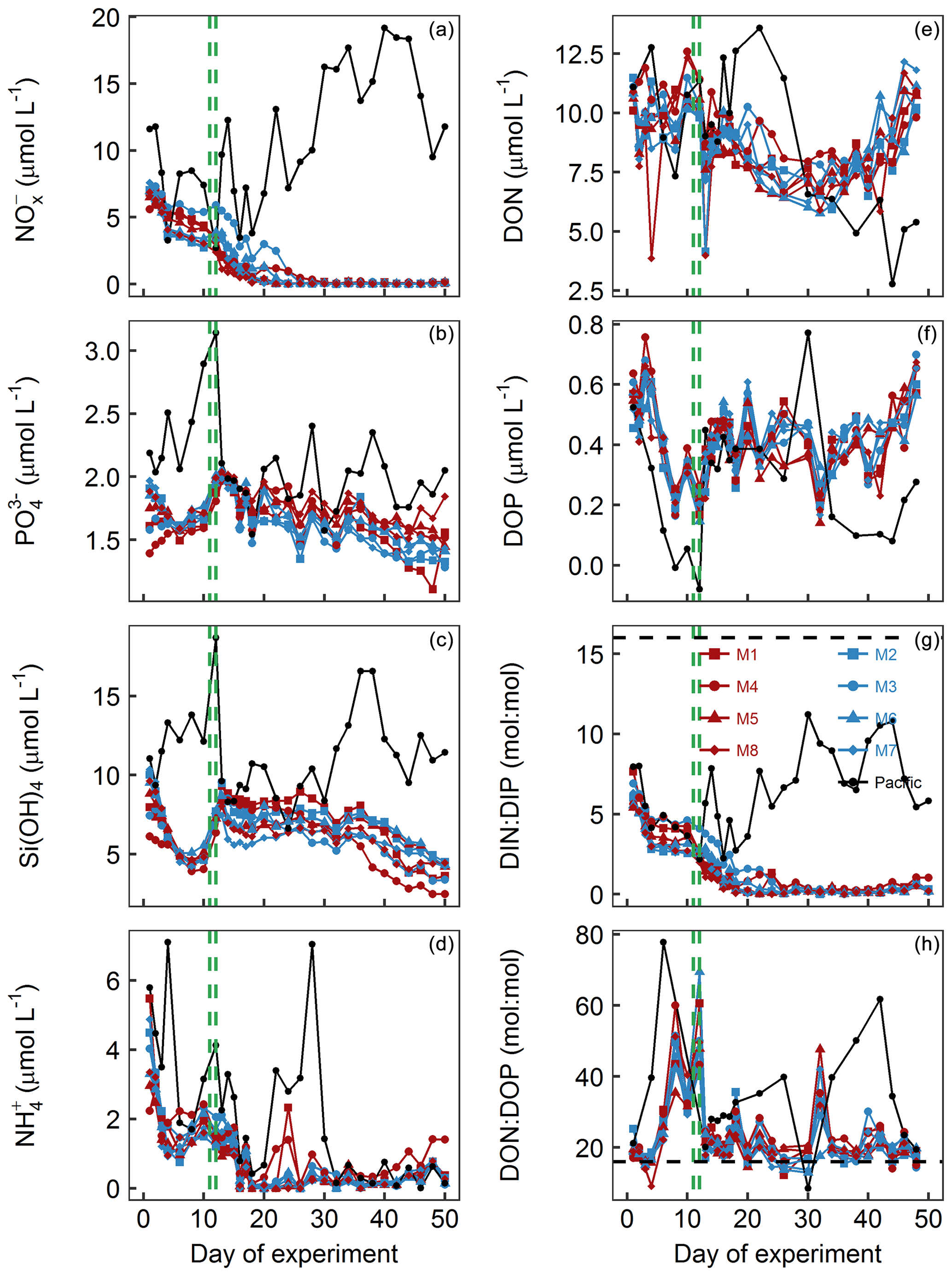
Figure 4Dissolved-inorganic-nutrient and dissolved-organic-nutrient concentrations and stoichiometries integrated over the 0–17 m depth range. The horizontal dashed black line in panel (g) displays the Redfield ratio of DIN : DIP =16. The green lines mark the days of OMZ water additions. (a) ${\mathrm{NO}}_{\mathrm{3}}^{-}$ + ${\mathrm{NO}}_{\mathrm{2}}^{-}$. (b) ${\mathrm{PO}}_{\mathrm{4}}^{\mathrm{3}-}$. (c) Si(OH)₄. (d) ${\mathrm{NH}}_{\mathrm{4}}^{+}$. (e) DON. (f) DOP. (g) DIN : DIP, i.e., $({\mathrm{NO}}_x^{-}+{\mathrm{NH}}_{\mathrm{4}}^{+})/{\mathrm{PO}}_{\mathrm{4}}^{\mathrm{3}-}$. (h) DON∕DOP.

Download

${\mathrm{PO}}_{\mathrm{4}}^{\mathrm{3}-}$ concentrations in the mesocosms were initially between 1.4 and 2 µmol L⁻¹ and converged to ∼1.6 µmol L⁻¹ in all mesocosms 5 d after the start of the experiment (Fig. 4b). The OMZ water contained 2.5 µmol L⁻¹ of ${\mathrm{PO}}_{\mathrm{4}}^{\mathrm{3}-}$ at both stations, so its addition increased the ${\mathrm{PO}}_{\mathrm{4}}^{\mathrm{3}-}$ concentrations in the mesocosms to ∼2 µmol L⁻¹ (Table 1). Afterwards, ${\mathrm{PO}}_{\mathrm{4}}^{\mathrm{3}-}$ decreased in all mesocosms but generally more in M2, M3, M6, and M7 (blue symbols in the figures) where slightly more ${\mathrm{NO}}_x^{-}$ was added through the OMZ water addition. ${\mathrm{PO}}_{\mathrm{4}}^{\mathrm{3}-}$ decreased during the second half of the experiment and was between 1.3 and 1.8 µmol L⁻¹ at the end. ${\mathrm{PO}}_{\mathrm{4}}^{\mathrm{3}-}$ was between 1.5 and 3.1 µmol L⁻¹ in the Pacific water and generally higher than in the mesocosms (Fig. 4b).

Si(OH)₄ concentrations in the mesocosms were initially between 6.1 and 10.3 µmol L⁻¹ and decreased in all mesocosms until Day 6 to values of between 4.5 and 5.1 µmol L⁻¹ (Fig. 4c). The OMZ water at station 1 and 3 contained 17.4 and 19.6 µmol L⁻¹ of Si(OH)₄, respectively, so their additions increased the concentrations to 7.5–9.5 µmol L⁻¹ inside the mesocosms (Table 1). Concentrations remained quite stable at this level until Day 26, after which they decreased in all mesocosms to 2.5–4.5 µmol L⁻¹ at the end of the study. Si(OH)₄ was between 6.6 and 18.7 µmol L⁻¹ in the Pacific water and generally higher than inside the mesocosms, except for a few days (Fig. 4c).

${\mathrm{NH}}_{\mathrm{4}}^{+}$ concentrations were initially between 2.2 and 5.5 µmol L⁻¹ and decreased to values <2 µmol L⁻¹ on days 2–3 (Fig. 4d). ${\mathrm{NH}}_{\mathrm{4}}^{+}$ increased thereafter (except for M8) to reach 1.5–2.4 µmol L⁻¹ on Day 10. After the OMZ addition, ${\mathrm{NH}}_{\mathrm{4}}^{+}$ concentrations (0.6 µmol L⁻¹) were slightly but significantly higher in M2, M3, M6, and M7, which received OMZ water from station 3 (blue symbols, Table 1). ${\mathrm{NH}}_{\mathrm{4}}^{+}$ concentrations decreased to values close to or below the limit of detection until Day 18. Concentrations remained at a low level but increased slightly by the end of the experiment to values of between 0.1 and 1.4 µmol L⁻¹. ${\mathrm{NH}}_{\mathrm{4}}^{+}$ concentrations ranged between the limit of detection and 7.1 µmol L⁻¹ in the Pacific water and coincidently showed a similar temporal pattern to that in the mesocosms except for the time between Day 10 and Day 20 when the concentrations were considerably higher (Fig. 4d).

DON concentrations in the mesocosms were initially between 10.1 and 11.5 µmol L⁻¹ and remained roughly within this range until the OMZ water addition. Afterwards, DON decreased to 6–7.9 µmol L⁻¹ on Day 30 but then increased almost exponentially until the end of the experiment (Fig. 4e). DON in the Pacific water was within a similar range to that in the mesocosms until the OMZ water addition but shifted to higher concentrations (10–13.6 µmol L⁻¹) from Day 16 to 22, followed by an abrupt decrease to 2.8–11.5 from Day 24 until the end of the experiment.

DOP concentrations in the mesocosms were initially between 0.45 and 0.63 µmol L⁻¹ but declined sharply to 0.16–0.25 µmol L⁻¹ on Day 8. DOP increased after the OMZ water addition to 0.22–0.38 µmol L⁻¹ (Table 1) and remained roughly at this level until Day 40, after which it began to increase to 0.56–0.7 µmol L⁻¹ towards the end of the experiment. There were several day-to-day fluctuations consistent among the mesocosms, and we cannot exclude the possibility that these are due to measurement inaccuracies (Fig. 4f). DOP in the Pacific water was initially similar to the mesocosms but decreased in the first week of the study to reach undetectable levels on Day 8. It increased, as in the mesocosms, on Day 13 and remained at 0.29–0.45 µmol L⁻¹ until Day 32. After a short peak of 0.77 µmol L⁻¹ on Day 34, DOP declined to 0.08–0.28 µmol L⁻¹ until the end of the experiment.

DIN : DIP (i.e., $({\mathrm{NO}}_x^{-}+{\mathrm{NH}}_{\mathrm{4}}^{+}):{\mathrm{PO}}_{\mathrm{4}}^{\mathrm{3}-}$) in the mesocosms was constantly below the Redfield ratio (i.e., 16), and its development largely resembled that of ${\mathrm{NO}}_x^{-}$ as the predominant nitrogen source (compare Fig. 4a and g). It was initially 5.4–7.7. After the OMZ water addition, DIN : DIP was significantly different between the two treatments (Table 1) because there was more DIN in the OMZ water added to M2, M3, M6, and M7 (blue symbols, Table 1). DIN : DIP decreased to 0.04–0.37 until Day 26 and remained at these low levels until the end of the experiment. DIN : DIP in the Pacific water was similar to the mesocosms until Day 13 but considerably higher (2.2–11.2) thereafter (Fig. 4g).

DON : DOP in the mesocosms was initially close to the Redfield ratio (i.e., 16) but increased to 29.2–40.4 until the OMZ water addition. Afterwards, DON : DOP declined to values slightly above the Redfield ratio and remained at this level until the end of the experiment. The occasional fluctuations towards higher values reflect the fluctuations in DOP (compare Fig. 4f and h). DON : DOP in the Pacific water was mostly above the Redfield ratio and generally higher than in the mesocosms. It was initially 21.1, increased to 77.6 on Day 6, and then rapidly declined to initial values. Afterwards, DON : DOP increased from 21.1 to 61.8 on Day 42 (with one exceptionally low value on Day 30) but then decreased to 19.5 at the end of the experiment (Fig. 4h).

Dissolved-iron (dissolved-Fe) concentrations were nonlimiting in all mesocosms with concentrations ranging from 3.1 to 17.8 nM (Table S1 in the Supplement; Bruland et al., 2005). The resolution of trace-metal clean sampling was insufficient for discussing the temporal trends in detail, although surface concentrations appeared to be lower on Day 48 (3.1-9.5 nM) than on Day 3 (range 5.7–10.8 nM). Dissolved-Fe concentrations in Pacific water on Day 48 (8.5 nM) were within the range of the mesocosms and also comparable to the nanomolar concentrations of dissolved Fe reported elsewhere in coastal surveys at shallow stations on the Peruvian Shelf (Bruland et al., 2005; Chever et al., 2015).

3.3 Phytoplankton development

Chl a concentrations in the mesocosms were initially between 2.3 and 4.9 µg L⁻¹ and declined to 1.4 to 2.4 µg L⁻¹ on Day 8 (Fig. 5a). Initially, high values of chl a were found mostly above 5 and below 15 m (Fig. 5b). The OMZ water addition increased chl a to 3.7–5.6 µg L⁻¹ (mesocosm-specific averages between Day 12 and Day 40) except for M3 where concentrations increased with a 1-week delay (3.4 µg L⁻¹ between Day 22 and Day 36) and M4 where concentrations remained at 1.6 µg L⁻¹ (average between Day 12 and Day 40; Fig. 5a). The chl a maximum remained in the upper 5 m in the week after the OMZ water addition, but shifted to the intermediate depth range of between 5 and 15 m thereafter and remained there until approximately Day 40. (Please note that the “quenching effect” can reduce in situ fluorometric chl a values especially near the surface so that absolute values may be biased; Holm-Hansen et al., 2000.) The exception was M4 where no such pronounced maximum was observed at intermediate depths (Fig. 5b). Chl a increased in all mesocosms, except for M4, to values of up to 38 µg L⁻¹ after Day 40 (Fig. 5a). This bloom occurred in the upper ∼5 m of the water column, due to surface eutrophication by defecating seabirds (Inca tern, Larosterna inca), who discovered the mesocosms as a suitable resting place (see Sect. 4.1). Chl a in the Pacific water was initially within the range enclosed inside the mesocosms, and concentrations increased to slightly higher values around the same time as in the mesocosms (Fig. 5). Throughout the study, chl a in the Pacific water was between 1.2 and 10.6 µg L⁻¹ with the chl a maxima always above 10 m (Fig. 5b).

Figure 5Chlorophyll a concentrations. (a) Average chl a concentrations over the entire water column (0–17 m) measured by HPLC. (b) Vertical distribution of chl a determined with the CTD fluorescence sensor on a logarithmic scale. The offset of the CTD sensor was corrected with the HPLC chl a data. Please note, however, that the quenching effect may have influenced in situ fluorometric chl a near the surface.

Download

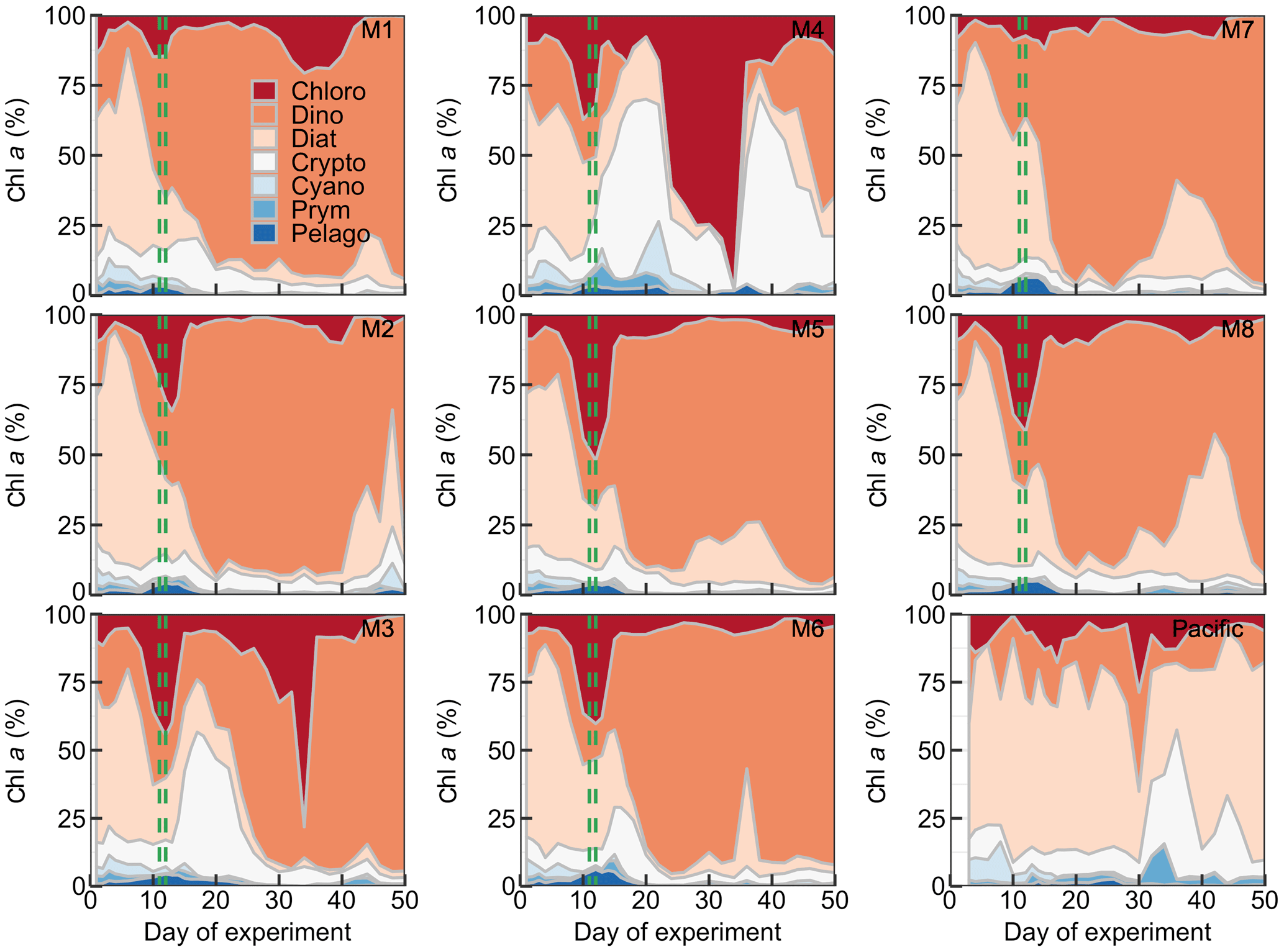
Figure 6Relative contribution of the different phytoplankton classes to the total chl a concentration. The mesocosm number is given on the top right of each subplot. The dashed green lines mark the days of OMZ water additions.

Download

The phytoplankton community composition was determined based on pigment concentration ratios using CHEMTAX (Figs. 6, S1). We distinguished between seven phytoplankton classes: Chloro-, Dino-, Crypto-, Cyano-, Prymnesio-, Pelago-, and Bacillariophyceae (i.e., diatoms) and use the word “dominant” in the following when a group contributes >50 % to chl a. Diatoms initially dominated the community and contributed 50 %–59 % of the total chl a concentration but declined after the start while Chlorophyceae (or Dinophyceae in M1 and M7) became more important. The other groups contributed mostly <25 % to chl a before the OMZ water addition. Diatoms contributed marginally to the chl a increase in the days after the addition. Instead, Dinophyceae became dominant in most mesocosms and contributed between 64 % and 76 % of the total chl a until the end of the experiment (range based on averages between Day 12 and Day 50 excluding M3 and M4). Imaging flow cytometry and microscopy revealed that the dinoflagellate responsible for this dominance was the large (∼60 µm) mixotrophic species Akashiwo sanguinea (Bernales et al., 2020). The A. sanguinea bloom was delayed by ∼10 d in M3, and they remained absent in M4 throughout the study. Cryptophyceae benefited from the absence of A. sanguinea and were the dominant group in M3 and M4 in the ∼10 d after the OMZ water addition (Fig. 6). Chlorophyceae were detectable in all mesocosms after the OMZ water addition with relatively low chl a contribution except for M1, M3, and M4 where they contributed up to 21 %, 78 %, and 98 %, respectively. Cyano-, Prymnesio-, and Pelagophyceae made hardly any contribution to chl a after the OMZ water addition (average <3 %) except for M4 where they were slightly more important (average =7 %). Diatoms formed blooms in some mesocosms after Day 30 where they became more important for relatively short times (M2, M5, M7, M8). The phytoplankton community composition in the Pacific water differed from that in the mesocosms. Here, diatoms were dominant throughout the study period except for two very short periods where either Chlorophyceae + Dinophyceae (Day 30) or Cyanophyceae + Cryptophyceae dominated (Day 36; Fig. 6).

3.4 Particulate matter pools and export fluxes

POC concentrations in the mesocosm water columns (POC_WC) were initially between 49 and 66 µmol L⁻¹ and declined following the OMZ water addition to 32–54 µmol L⁻¹ on Day 16. POC_WC started to increase after Day 16, and POC_WC reached a new steady state of 75–116 µmol L⁻¹ between Day 24 and Day 44. Exceptions were M3 and M4 where the increase either was delayed (M3) or did not take place at all (M4). POC_WC increased rapidly at the end of the experiments (Fig. 7a). POC_WC in the Pacific water was between 34 and 72 µmol L⁻¹ between Day 0 and Day 24 and decreased thereafter to values of between 27 and 55 µmol L⁻¹ (Fig. 7a). The accumulation of POC in the sediment traps (ΣPOC_ST) was surprisingly constant over the course of the study, with an average rate of 1.06 µmol POC L⁻¹ d⁻¹ (Fig. 7c).

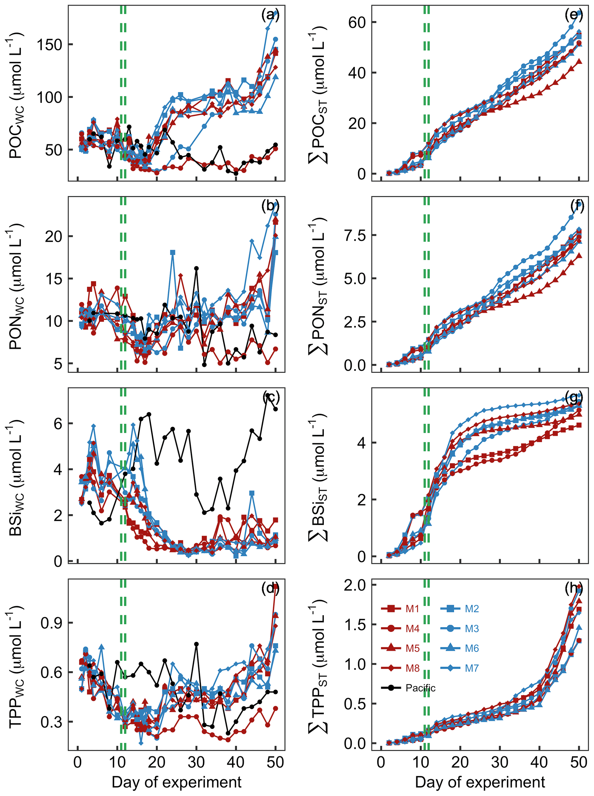
Figure 7Particulate organic matter concentrations and cumulative export. Shown in panels (a)–(d) are concentrations averaged over the entire water column (0–17 m). Shown in panels (e)–(h) are cumulative export fluxes of particulate matter over the course of the study. The green lines mark the days of OMZ water additions.

Download

PON_WC concentrations in the mesocosms were initially between 9.2 and 11.9 µmol L⁻¹ and declined after the OMZ water addition to 6.2–10.3 µmol L⁻¹ on Day 16. The increase in PON_WC to 8.4–18.1 µmol L⁻¹ during days 17–24 was much less pronounced compared to POC_WC (compare Fig. 8a and b). Furthermore, M3 and M4 were not markedly different from the other mesocosms during this period. However, M4 was the only mesocosm where PON_WC declined profoundly after Day 30 and remained at a lower level until the end. PON_WC in all other mesocosms remained at 5–18.1 µmol L⁻¹ between Day 24 and Day 42 but increased markedly towards the end of the experiment (Fig. 7b). PON_WC in the Pacific water varied between 7.9 and 16.2 µmol L⁻¹ between Day 0 and Day 30 and between 4.8 and 9.6 µmol L⁻¹ from Day 32 until the end of the experiment. ΣPON_ST accumulation was, like ΣPOC_ST, relatively constant over time, averaging at a rate of 0.15 µmol PON L⁻¹ d⁻¹ (Fig. 7d).

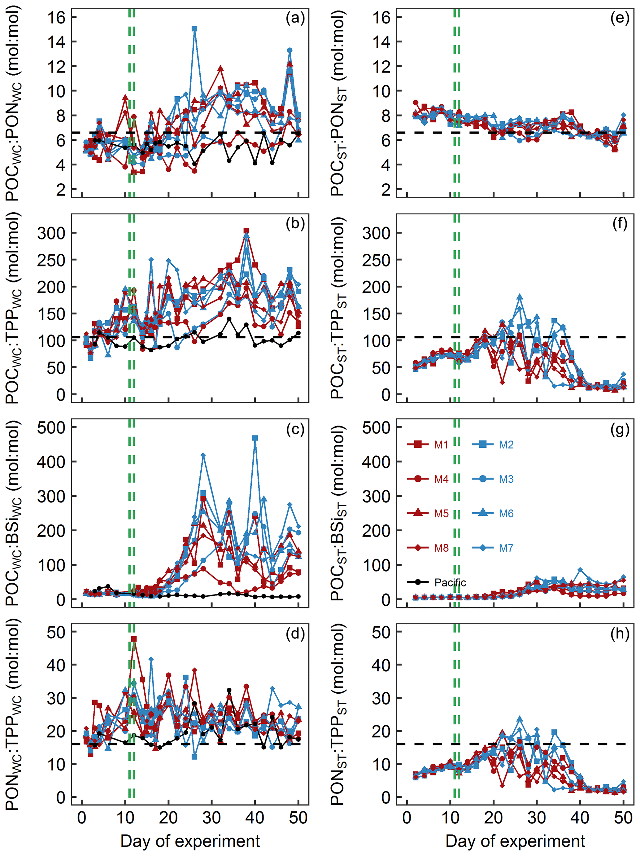
Figure 8Particulate matter stoichiometry. Shown in panels (a)–(d) are elemental ratios of particulate matter in the water column. Panels (e)–(h) show the same ratios but for particulate matter collected in the sediment traps. The horizontal dashed black lines display Redfield ratios (i.e., POC : PON =6.6, POC : TPP =106, PON : TPP =16). The vertical dashed green lines mark the days of OMZ water additions.

Download

BSi_WC concentrations in the mesocosms were initially 2.5–3.7 µmol L⁻¹ but decreased after the OMZ water addition to 0.4–0.8 µmol L⁻¹ on Day 26. They remained at these low levels until the end of the experiment with smaller peaks in some mesocosms due to minor diatom blooms (compare Figs. 8d and 6). The BSi_WC development in the Pacific water was very different from that in the mesocosms. Here, BSi_WC was initially lower but increased to 6.4 between Day 0 and Day 18. Afterwards it decreased for a short period but increased again towards the end of the experiment (Fig. 7c). ΣBSi_ST accumulation was high in the first 3 weeks when diatoms were still relatively abundant (0.22 µmol BSi L⁻¹ d⁻¹) but very low thereafter (0.04 µmol BSi L⁻¹ d⁻¹; Fig. 7g).

TPP_WC concentration decreased from 0.49–0.67 on Day 0 to 0.27–0.36 µmol L⁻¹ on Day 12 and remained around this level until Day 20. Afterwards, TPP_WC increased rapidly in all mesocosms except M4 to a new level of between 0.37 and 0.65 µmol L⁻¹ until Day 24. TPP_WC increased almost exponentially in all mesocosms from Day 38 until the end of the experiment. TPP_WC was variable in the Pacific water but generally higher between Day 0 and Day 30 (0.37–0.77 µmol L⁻¹) than from Day 32 until the end (0.28–0.43 µmol L⁻¹; Fig. 7d). ΣTPP_ST accumulation was constant at a rate of about 0.015 µmol TPP L⁻¹ d⁻¹ until Day 40 but increased sharply to 0.1 µmol TPP L⁻¹ d⁻¹ thereafter (Fig. 7h).

3.5 Particulate organic matter stoichiometry

POC_WC : PON_WC in the mesocosms was initially between 5.1 and 5.8 and thus below the Redfield ratio (6.6). POC_WC : PON_WC remained at approximately these values until some days after the OMZ water addition when it increased to 7.9–11.8 in all mesocosms except for M3 and M4. In M3, the increase was delayed by about a week, whereas in M4 it remained at a lower level of 3.5–8.3 throughout the experiment. POC_WC : PON_WC decreased during the last 10 d of the study in all mesocosms except for M4 (Fig. 8a). POC_WC : PON_WC in the Pacific water remained at around the initial value of 6 throughout the study (Fig. 8a). POC_ST : PON_ST ratios were considerably less variable than POC_WC : PON_WC. They were initially 7.9–9 and therefore higher than in the water column but decreased steadily over the course of the experiment, so they became lower than in the water columns in all mesocosms except M4 from around Day 30 onwards (Fig. 8e).

POC_WC : TPP_WC in the mesocosms was initially close to the Redfield ratio (i.e., 106) but increased quite steadily up to 182–304 until Day 38 except for a short decline after the OMZ water addition. The increase was also apparent in M3 and M4, although it was less pronounced and there was little change in the 2 weeks after the OMZ water addition. POC_WC : TPP_WC decreased from days 40 to 44 when it reached values of between 125 and 177 and remained approximately there (Fig. 8b). POC_WC : TPP_WC was much more stable in the Pacific water and relatively close to the Redfield ratio throughout the experiment (Fig. 8b). POC_ST : TPP_ST was always considerably lower than POC_WC : TPP_WC (compare Fig. 8b and f). POC_ST : TPP_ST increased in all mesocosms from initially 46–59 to 88–117 on Day 18, after which it varied widely between mesocosms. POC_ST : TPP_ST converged to a much narrower and very low value of between 7 and 42 from Day 40 until the end (Fig. 8f).

POC_WC : BSi_WC in the mesocosms was between 8 and 34 from the start until Day 16 but increased substantially to 88–418 until Day 28 and remained at a high level until the end of the experiment. The increase in POC_WC : BSi_WC was slightly delayed in M3 and generally less pronounced in M4 (Fig. 8c). POC_WC : BSi_WC in the Pacific water remained at a low level of 7–38 throughout the experiment (Fig. 8c). POC_ST : BSi_ST also increased from 4–7 (until Day 16) to 4–86 (Day 18 until end) but was generally much lower than in the water column throughout the study (compare Fig. 8c and g).

PON_WC : TPP_WC in the mesocosms was initially close to the Redfield ratio (i.e., 16) but increased to 19–36 until the OMZ water addition. Afterwards, PON_WC : TPP_WC fluctuated around this elevated value with a slight tendency to decrease until the end of the experiment (Fig. 8d). PON_WC : TPP_WC in the Pacific water was 15–20 and thus mostly above the Redfield ratio until Day 24, but the positive offset increased to 15–32 thereafter (Fig. 8d). PON_ST : TPP_ST was considerably lower than PON_WC : TPP_WC and below the Redfield ratio almost throughout the experiment. Its temporal development resembled the development of POC_ST : TPP_ST (compare Fig. 8f and h). It increased steadily from 6–7 at the beginning to 12–15 on Day 18, followed by a phase of large variability between mesocosms until Day 40. PON_ST : TPP_ST declined to 1–5 afterwards and remained at this low range level until the end of the experiment (Fig. 8h).

4.1 Small-scale variability, OMZ water signature similarities, and defecating seabirds – lessons learned from a challenging in situ mesocosm study during coastal El Niño 2017

A key prerequisite to comparing different mesocosm treatments is the enclosure of identical water masses in all mesocosms at the beginning of the study (Spilling et al., 2019). Unfortunately, this was not particularly successful in our experiment as can be seen for example in the differences in initial inorganic nutrient concentrations (Fig. 4). Although our procedure of lowering the mesocosms bags and allowing for several days of water exchange does not exclude heterogeneity entirely (Bach et al., 2016a; Paul et al., 2015; Schulz et al., 2017), it was not as pronounced during our previous studies as experienced in Peru. The reason for this was likely the inherent small-scale patchiness of physicochemical conditions in the near coastal parts of EBUS (Chavez and Messié, 2009). We encountered small foamy patches with an H₂S smell indicative of submesoscale upwelling of anoxic waters, ultra-dense meter-sized swarms of zooplankton coloring the water red, and brownish filaments of discharging river water from the nearby Rímac River which carried large amounts of water due to flooding during the coastal El Niño (Garreaud, 2018). In such extraordinarily variable conditions, the mesocosms should be deployed and sealed in a very short time when conditions in the study site are relatively homogeneous. Alternatively, larger variability can be taken into account by increasing the number of replicates, but this was not feasible in our case due to the costs of a mesocosm unit of this size.

A major motivation for our experiment was to investigate how plankton communities in the coastal upwelling system off Peru would respond to upwelling of OMZ waters with different N : P signatures (question 2 mentioned in the introduction). The rationale for this was that projected spatial extensions of OMZs and intensification of their oxygen depletion in a future ocean could enhance the N deficit in the study region with strong implications for ecological and biogeochemical processes (García-Reyes et al., 2015; Stramma et al., 2010). However, there was unusually little bioavailable inorganic N in both OMZ water masses so the differences in inorganic N : P signatures between the two treatments were significant but small (Table 1; Fig. 4g). Because the differences were small, we decided to focus the present paper on the analyses of temporal developments. However, other publications in this special issue on the Peru mesocosm project will also have a closer look into treatment differences.

Another complicating factor during the experiment was the presence of Inca terns (Larosterna inca) – an abundant seabird species in the study region that began to roost in the limited space between the antibird spikes we installed on the mesocosm roofs (see video by Boxhammer et al., 2019). Until Day 36, their presence was occasional, but it increased profoundly thereafter. Additional bird scarers installed on Day 37 were unfortunately ineffective, and during the last 2 weeks of the study, we often counted more than 10 individuals on each mesocosm. It was evident that they defecated into the mesocosms as there was excrement on the inner side of the bags above the surface.

To get a rough estimate of the nutrient inputs through this “orni-eutrophication” in the mesocosms, we first assumed that the increase in TPP export after Day 40 is sinking excrement P (Fig. 7h). This assumption is reasonable because ${\mathrm{PO}}_{\mathrm{4}}^{\mathrm{3}-}$ was far from limiting and did not show any noticeable change in concentration during this time (Fig. 4b). Correcting the TPP export after Day 40 (0.1 µmol L⁻¹ d⁻¹) with the background value of the time before (0.015 µmol L⁻¹ d⁻¹) yields 0.085 µmol L⁻¹ d⁻¹ of P inputs from Inca terns. This converts to 1.15 µmol L⁻¹ d⁻¹ of N inputs, assuming a 13.5 : 1 N : P stoichiometry as reported for South American seabird excrements (Otero et al., 2018). This estimation is in reasonable agreement with the observed PON_WC + DON + ${\mathrm{NH}}_{\mathrm{4}}^{+}$ increase of 5.2–17 µmol L⁻¹ observed from days 40 to 50 (Figs. 4d, e, and 8b; note that PON_ST as well as ${\mathrm{NO}}_x^{-}$ is considered to remain constant in this approximation; Figs. 4a and 8f). These N inputs into the mesocosms are at least 5 orders of magnitude higher than what seabirds typically add to the water column of the Pacific in this region (Otero et al., 2018). Accordingly, the phytoplankton bloom that occurred in the upper 5 m after Day 40 was fueled by orni-eutrophication. While this certainly is an undesired experimental artifact, it had some advantages for interpreting the data as is highlighted in Sect. 4.2.1.

The coastal El Niño that climaxed during our experiment (Garreaud, 2018) is the last peculiarity we want to highlight in this section. Coastal El Niño events are rare with similar phenology to usual El Niño events that are regionally restricted to the far eastern Pacific. The last such event of similar strength occurred in 1925 (Takahashi and Martínez, 2019). Surface water temperatures (upper 5 m) are mostly below 20 ^∘C in this region during non El Niño years (Graco et al., 2017) but were 20–25 ^∘C for most of the time during our study (Fig. 3a). This may have influenced metabolic processes of plankton and also enhanced stratification. Thus, it is possible that the observed conditions discussed in the following sections may not be entirely representative for the more common non-El Niño conditions.

4.2 Factors controlling production and export

Messié and Chavez (2015) identified light, macronutrient, and iron supply and transport processes (e.g., subduction) to be the key factors regulating primary and export production in EBUS. We can immediately exclude transport processes and iron concentration from having played a major role in our study. Transport processes above the microscale are excluded in mesocosms. Iron concentrations are elevated to nanomolar concentrations in shallow waters along the Peruvian shelf (Bruland et al., 2005) generally leading to a sharp contrast between Fe-limited (or co-limited) offshore ecosystems and Fe-replete conditions in highly productive inshore regions (Browning et al., 2018; Hutchins et al., 2002). Dissolved-Fe concentrations were verified to be high in the mesocosms both in surface and subsurface waters throughout the experiment (days 3, 17, 48; Table S1) confirming that Fe was replete compared to N. Thus, our subsequent discussion will only consider light and macronutrients (mostly N because P was also replete) as well as phytoplankton community composition as controlling factors of production and export.

4.3 Particulate C : N : P : Si stoichiometry in the mesocosms

4.3.3 C : Si

POC_WC : BSi_WC was initially low (Fig. 8c), indicative of a diatom-dominated community (Brzezinski, 1985). The increase in POC_WC : BSi_WC about a week after the OMZ water addition coincides roughly with the depletion of ${\mathrm{NO}}_x^{-}$ even though Si(OH)₄ was still available in higher concentrations (compare Figs. 4a, c and 9c). This suggests that the change from diatom to dinoflagellate predominance was triggered by N and not Si limitation. The POC_WC : BSi_WC increase is lower in M4 where A. sanguinea was absent, underlining that this species was a key player driving the trend in the other mesocosms.

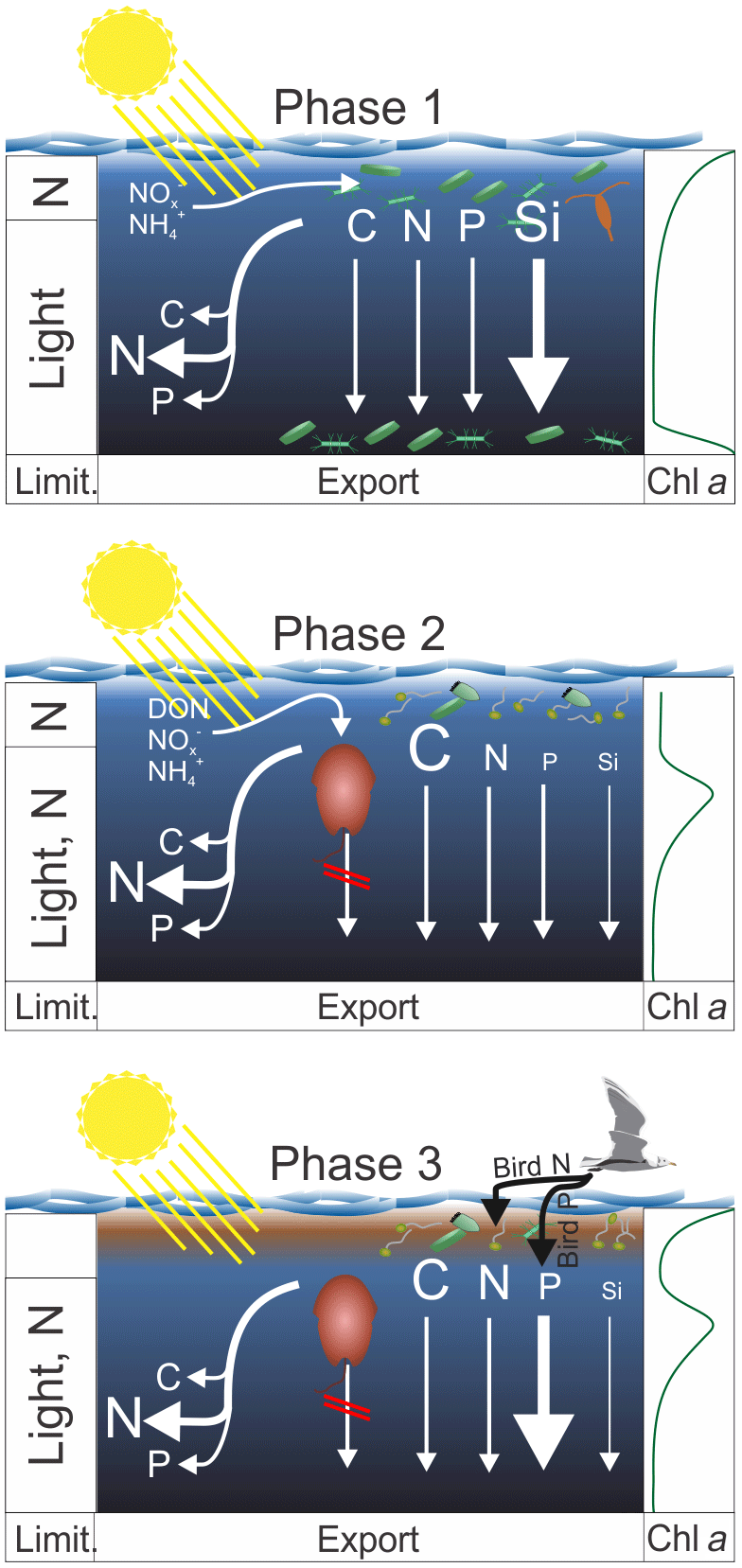
Figure 9Synthesis graphic. The text in Sect. 5 functions as an extended figure caption and should be read to fully understand processes illustrated in this graphic. The left column indicates the factors limiting organic matter production in the upper ∼5 m and below. The arrows on the left identify which elements were remineralized preferentially during sinking. The arrows on the right indicate the export flux of these elements. In both cases strength is indicated by the arrow and letter sizes. The column on the right shows the approximate chl a profile during the three phases. The brown phytoplankton drawn in pictures of Phase 2 and 3 illustrates A. sanguinea.

Download

POC_ST : BSi_ST also increased after the OMZ water addition but the increase was considerably less pronounced than for POC_WC : BSi_WC. Once again, the explanation for this is the persistence of A. sanguinea which maintains the high signal in the water column but does not transfer it to the exported material because it did not sink out during the experiment.