the Creative Commons Attribution 4.0 License.
the Creative Commons Attribution 4.0 License.
 | 22 Jan 2019
Description and evaluation of the Community Ice Sheet Model (CISM) v2.1
Stephen F. Price
Matthew J. Hoffman
Gunter R. Leguy
Andrew R. Bennett
Sarah L. Bradley
Katherine J. Evans
Jeremy G. Fyke
Joseph H. Kennedy
Mauro Perego
Douglas M. Ranken
William J. Sacks
Andrew G. Salinger
Lauren J. Vargo
Patrick H. Worley
We describe and evaluate version 2.1 of the Community Ice Sheet Model (CISM). CISM is a parallel, 3-D thermomechanical model, written mainly in Fortran, that solves equations for the momentum balance and the thickness and temperature evolution of ice sheets. CISM's velocity solver incorporates a hierarchy of Stokes flow approximations, including shallow-shelf, depth-integrated higher order, and 3-D higher order. CISM also includes a suite of test cases, links to third-party solver libraries, and parameterizations of physical processes such as basal sliding, iceberg calving, and sub-ice-shelf melting. The model has been verified for standard test problems, including the Ice Sheet Model Intercomparison Project for Higher-Order Models (ISMIP-HOM) experiments, and has participated in the initMIP-Greenland initialization experiment. In multimillennial simulations with modern climate forcing on a 4 km grid, CISM reaches a steady state that is broadly consistent with observed flow patterns of the Greenland ice sheet. CISM has been integrated into version 2.0 of the Community Earth System Model, where it is being used for Greenland simulations under past, present, and future climates. The code is open-source with extensive documentation and remains under active development.


As mass loss from the Greenland and Antarctic ice sheets has accelerated (Shepherd et al., 2012; Church et al., 2013; Hanna et al., 2013; Shepherd et al., 2017), climate modelers have recognized the importance of dynamic ice sheet models (ISMs) for predicting future mass loss and sea level rise (Vizcaino, 2014). Meanwhile, ISMs have become more accurate and complex in their representation of ice flow dynamics. Early ISMs used either the shallow-ice approximation (SIA; Hutter, 1983) or the shallow-shelf approximation (SSA; MacAyeal, 1989). The SIA, which assumes that vertical shear stresses are dominant, is valid for slow-moving ice sheet interiors, whereas the SSA, which assumes that flow is dominated by lateral and longitudinal stresses in the horizontal plane, is valid for floating ice shelves. Neither approximation is valid for ice streams and outlet glaciers where both vertical shear and horizontal plane stresses are important. Advanced ISMs developed in recent years solve the Stokes equations or various higher-order approximations (Pattyn et al., 2008; Schoof and Hindmarsh, 2010). Among the models that solve Stokes or higher-order equations, or otherwise combine features of the SIA and SSA, are the Parallel Ice Sheet Model (PISM; Bueler and Brown, 2009; Winkelmann et al., 2011), the Ice Sheet System Model (ISSM; Larour et al., 2012), the Penn State Model (Pollard and DeConto, 2012), BISICLES (Cornford et al., 2013), Elmer-Ice (Gagliardini et al., 2013), and MPAS-Albany Land Ice (MALI; Tezaur et al., 2015; Hoffman et al., 2018). Higher-order models have performed well for standard test cases (Pattyn et al., 2008, 2012) and have been applied to many scientific problems.
Here, we describe and evaluate the Community Ice Sheet Model (CISM) version 2.1, a higher-order model that evolved from the Glimmer model (Rutt et al., 2009). The current name reflects the model's evolution as a component of the Community Earth System Model (CESM; Hurrell et al., 2013). Like Glimmer, CISM is written mainly in Fortran 90 and its extensions, to maximize efficiency and to simplify coupling to climate models. Glimmer, however, is a serial SIA model, whereas CISM is a parallel model that solves not only the SIA but also higher-order Stokes approximations.
CISM development was guided by the following goals:
-
The model should be well documented and easy to install and run on a variety of platforms, ranging from laptops to local clusters to high-performance supercomputers.
-
It should solve a range of Stokes approximations, including the SIA, SSA, and higher-order approximations. Velocity solvers for these approximations are included in a new dynamical core called Glissade. (The dynamical core, or “dycore”, is the part of the model that solves equations for conservation of mass, energy, and momentum.)
-
It should remain backward-compatible with Glimmer, allowing continued use of the older Glide SIA dycore.
-
It should be well verified for standard test cases such as the Ice Sheet Model Intercomparison Project for Higher-Order Models (ISMIP-HOM) (Pattyn et al., 2008), with a user-friendly verification framework.
-
It should run efficiently – supporting whole-ice-sheet applications even on small platforms – and should scale to hundreds of processor cores, enabling century- to millennial-scale simulations with higher-order solvers at grid resolutions of ∼5 km or finer.
-
It should support not only stand-alone ice sheet simulations but also coupled applications in which fields are exchanged with a global climate or Earth system model (CESM in particular).
-
It should support simulations of the Greenland ice sheet, a scientific focus of CESM. Support for Antarctic applications is deferred to future model releases and publications.
-
The code should be open-source, with periodic public releases.
Many of these features were present in CISM v.2.0, which was released in 2014 (Price et al., 2015).
Changes between versions 2.0 and 2.1 have been made primarily to support robust, accurate, and efficient Greenland ice sheet simulations, both as a stand-alone model and in CESM. These changes include a depth-integrated higher-order velocity solver (Sect. 3.1.4), new parameterizations of basal sliding (Sect. 3.4), iceberg calving (Sect. 3.5), and sub-ice-shelf melting (Sect. 3.6), a new build-and-test structure (Sect. 4.6), and many improvements in model numerics.
We begin with an overview of CISM, including the core model and its testing and coupling infrastructure (Sect. 2). We then describe the model dynamics and physics, focusing on the new Glissade dycore (Sect. 3). To verify the model, we present results from standard test cases (Sect. 4). We then present results from long spin-ups of the Greenland ice sheet, with and without floating ice shelves (Sect. 5). Finally, we summarize the model results and suggest directions for future work (Sect. 6).
CISM is a numerical model – a collection of software libraries, utilities, and drivers – used to simulate ice sheet evolution. It is modular in design and is coded mainly in standard-compliant Fortran 90/95. CISM consists of several components:
- cism_driver
-
is the high-level driver (i.e., the executable) that is used to run the stand-alone model in all configurations, including idealized test cases with simplified climate forcing, as well as model runs with realistic geometry and climate forcing data.
- Glide
-
is the serial dycore based on shallow-ice dynamics. Glide solves the governing conservation equations and computes ice velocities, internal ice temperature, and ice geometry evolution. Apart from minor changes, this is the same dycore used in Glimmer and described by Rutt et al. (2009). It will not be discussed further here.
- Glissade
-
is the dycore that solves higher-order approximations of the Stokes equations for ice flow. Glissade, unlike Glide, is fully parallel in order to take advantage of multiprocessor, high-performance architectures. It is described in detail in Sect. 3.
- Glint
-
is the original climate model interface for Glimmer. Glint allows the core ice sheet model to be coupled to a global climate model or any other source of time-varying climate data on a lat–long grid. Glint computes the surface mass balance (SMB) on the ice sheet grid using a positive-degree-day (PDD) scheme.
- Glad
-
is a lightweight climate model interface that has replaced Glint in CESM. The CESM coupler supports remapping and downscaling between general land-surface grids and ice sheet grids, and thus is able to send CISM an SMB that is already downscaled. The Glad interface simply sends and receives fields on the ice sheet grid, accumulating and averaging as needed based on the ice dynamic time step and the coupling interval.
- Test cases
-
are provided for the Glide and Glissade dynamical cores. These are used to confirm that the model is working as expected and to provide a range of simple model configurations from which new users can learn about model options and create their own configurations. CISM test cases are described in Sect. 4.
- Shared code
-
consists of modules shared by different parts of the code. Examples include modules for defining derived types, physical constants, and model parameters, and modules that parse CISM configuration files and handle data input/output (I/O).
In order to reduce development effort, CISM runs on a structured rectangular grid and thus lacks the flexibility of models that run on variable-resolution or adaptive meshes (e.g., ISSM and BISICLES). Although CISM includes several common Stokes approximations, it does not solve the more complex “full Stokes” equations (Pattyn et al., 2008).
CISM is distributed as source code and therefore requires a reasonably complete build environment to compile the model. For UNIX- and LINUX-based systems, the CMake (http://www.cmake.org/, last access: 20 January 2019) system is used to build the model. Sample build scripts for a number of standard architectures are included, as are working build scripts for a number of high-performance-computing architectures including Cheyenne (NCAR Computational and Information Systems Laboratory), Titan (Oak Ridge Leadership Computing Facility), Edison (National Energy Research Scientific Computing Center), and Cartesius (the Dutch national supercomputer).
The source code can be obtained by downloading a released version from the CISM website or by cloning the code from a public git repository; see Sect. . In either case, a Fortran 90 compiler is required. Other software dependencies include the NetCDF library (https://www.unidata.ucar.edu/software/netcdf/, last access: 20 January 2019) (used for data I/O) and a Python (http://www.python.org, last access: 20 January 2019) distribution (used to analyze dependencies and to automatically generate parts of the code) with several specific Python modules. Parallel builds require Message Passing Interface (MPI), and users desiring access to Trilinos packages (Heroux et al., 2005) will need to build Trilinos and then link it to CISM. Finally, CMake and Gnu Make are needed to compile the code and link to the various third-party libraries. The CISM documentation contains detailed instructions for downloading and building the code.
CISM is run by specifying the names of the executable (usually cism_driver) and a configuration file. Typically, the configuration file includes the input and output filenames, the grid dimensions, the time step and length of the run, the dycore (Glide or Glissade), and various options and parameter values appropriate for a given application. If not set in the config file, each option or parameter takes a default value. Supported options are described in the model documentation.
Multiple input, forcing, and output files can be specified, containing any subset of a large number of global scalars and fields (1-D, 2-D, and 3-D). If a given field is “loadable” and is present in the input file, it is read automatically at startup; otherwise, it is set to a default value. Loadable fields include the initial ice thickness and temperature, bedrock topography, surface mass balance, surface air temperature, and geothermal heat flux. Forcing files are input files that are read at every time step (not just at initialization) so that time-dependent forcing can be applied during a simulation.
Each output file includes a user-chosen set of variables (listed in the configuration file) and can contain multiple time slices, written at any frequency. A special kind of I/O file is the restart file, which includes all the fields needed to restart the model exactly. Whatever configuration options are chosen, model results are exactly reproducible (i.e., bit for bit) for a given computer platform and processor count, regardless of how many times a simulation is stopped and restarted.
Some basic information is sent to standard output during the run, and more verbose output is written at regular intervals to a log file. The log file lists the options and parameter values chosen for the run and also notes the simulation time when CISM reads or writes I/O. In addition, the log file includes diagnostic information about the global state of the model (e.g., the total ice area and volume, total surface and basal mass balance, and maximum surface and basal ice speeds), along with vertical profiles of ice speed and temperature for a user-chosen grid point.
CISM2.1 has been implemented in CESM version 2.0, released in June 2018. Earlier versions of CESM supported one-way forcing of the Greenland ice sheet (using SIA dynamics) by the SMB computed in CESM's land model (Lipscomb et al., 2013). CESM2.0 extends this capability by supporting conservative, interactive coupling between ice sheets and the land and atmosphere. Coupling of ice sheets with the ocean is not yet supported but is under development. CESM2.0 does not have an interactive Antarctic ice sheet, in part because of the many scientific and technical issues associated with ice sheet–ocean coupling. However, CISM2.1 includes many of the features needed to simulate marine ice sheets, and a developmental model version (including a grounding-line parameterization to be included in a near-future code release) has been used for Antarctic simulations.
CISM includes a parallel, higher-order dynamical core called Glissade, which solves equations for conservation of momentum (i.e., an appropriate approximation of Stokes flow), mass, and internal energy. Glissade numerics differ substantially from Glide numerics:
-
Velocity: Glide solves the SIA only, but Glissade can solve several Stokes approximations, including the SIA, SSA, a depth-integrated higher-order approximation based on Goldberg (2011), and a 3-D higher-order approximation based on Blatter (1995) and Pattyn (2003). Glide uses finite differences, whereas the Glissade velocity solvers use finite-element methods.
-
Temperature: To evolve the ice temperature, Glide solves a prognostic equation that incorporates horizontal advection as well as vertical heat diffusion and internal dissipation. In Glissade, temperature advection is handled by the transport scheme, and a separate module solves for vertical diffusion and internal dissipation in each column.
-
Mass and tracer transport: Glide solves an implicit diffusion equation for mass transport, incorporating shallow-ice velocities. Glissade solves explicit equations for horizontal transport of mass (i.e., ice thickness) and tracers (e.g., ice temperature) using either an incremental remapping scheme (Lipscomb and Hunke, 2004) or a simpler first-order upwind scheme. Horizontal transport is followed by vertical remapping to terrain-following sigma coordinates.
Glissade numerics are described in detail below.
3.1 Velocity solvers
Glissade computes the ice velocity by solving approximate Stokes equations, given the surface elevation, ice thickness, ice temperature, and relevant boundary conditions. Section 3.1.1 describes the solution method for the Blatter–Pattyn (BP; Blatter, 1995; Pattyn, 2003) approximation, which is the most sophisticated and accurate solver in CISM. Subsequent sections discuss simpler approximations.
3.1.1 Blatter–Pattyn approximation
The basic equations of the Blatter–Pattyn approximation are
where u and v are the components of horizontal velocity, η is the effective viscosity, ρi is the density of ice (assumed constant), g is gravitational acceleration, s is the surface elevation, and are 3-D Cartesian coordinates. These and other variables and parameters used in CISM are listed in Tables 1 and 2 for reference. In each equation, the three terms on the left-hand side (LHS) describe gradients of longitudinal stress, lateral shear stress, and vertical shear stress, respectively, and the right-hand side (RHS) gives the gravitational driving force. The longitudinal and lateral shear stresses together are sometimes called membrane stresses (Hindmarsh, 2006). Neglecting membrane stress gradients leads to the much simpler SIA, and neglecting vertical shear stress gradients leads to the SSA.
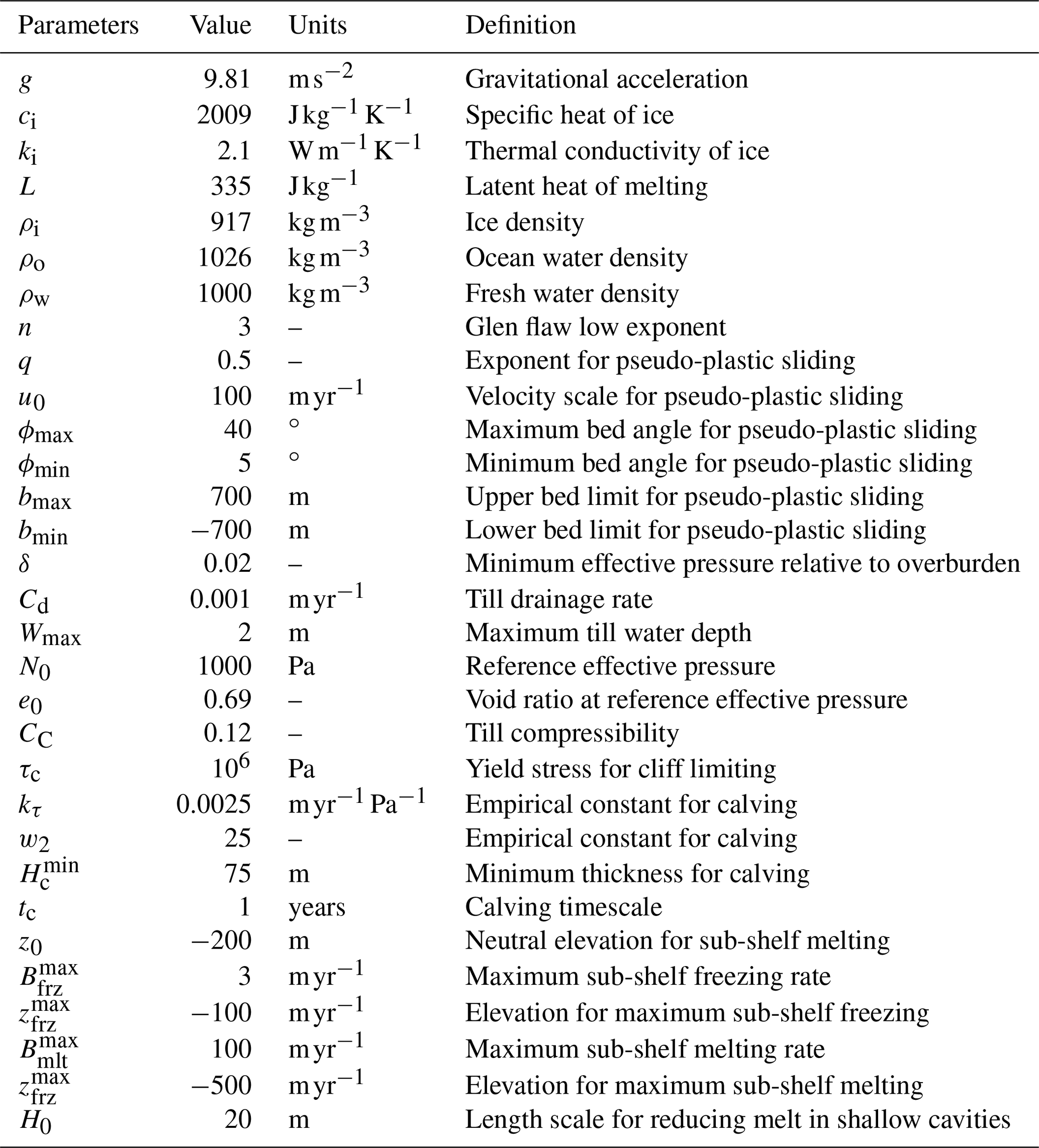
Table 2Model constant and parameter values used for simulations described in the text. The calving and sub-shelf melting parameters are used only for simulations with ice shelves; other parameters are used for all Greenland simulations.
The equations are discretized on a structured 3-D mesh. In the map plane, the mesh consists of rectangular cells, each with four vertices. The nz vertical levels of the mesh are based on a terrain-following sigma coordinate system, with , where H is the ice thickness. Each cell layer is treated as a 3-D hexahedral element with eight nodes. (In other words, cells and vertices are defined to lie in the map plane, whereas elements and nodes live in 3-D space.) Scalar 2-D fields such as H and s are defined at cell centers, and 3-D scalars such as the ice temperature T lie at the centers of elements. Gradients of 2-D scalars (e.g., the surface slope ∇s) live at vertices. The velocity components u and v are 3-D fields defined at nodes.
For problems on multiple processors, a cell or vertex (and the associated elements and nodes in its column) may be either locally owned or part of a computational halo. Each processor is responsible for computing u and v at its locally owned nodes. Any cell that contains one or more locally owned nodes and has H exceeding a threshold thickness (typically 1 m) is considered dynamically active, as are the elements in its column. Likewise, any vertex of an active cell is active, as are the nodes in its column.
The effective viscosity η is defined in each active element by
where A is the temperature-dependent rate factor in Glen's flow law (Glen, 1955), and is the effective strain rate, given in the BP approximation by
where the components of the symmetric strain rate tensor are
The rate factor A is given by an Arrhenius relationship:
where T* is the absolute temperature corrected for the dependence of the melting point on pressure (, with T in Kelvin), a is a temperature-independent material constant from Paterson and Budd (1982), Q is the activation energy for creep, and R is the universal gas constant.
The coupled partial differential equations (PDEs) (1) are discretized using the finite-element method (e.g., Hughes, 2000; Huebner et al., 2001). This method is more often applied to unstructured grids but was chosen for CISM's rectangular grid because of its robustness and natural treatment of boundary conditions (Dukowicz et al., 2010). The PDEs, with appropriate boundary conditions, are converted to a system of algebraic equations by dividing the full domain into subdomains (i.e., hexahedral elements), representing the velocity solution on each element, and integrating over elements. The solution is approximated as a sum over trilinear basis functions φ. Each active node is associated with a basis function whose value is φ=1 at that node, with φ=0 at all other nodes. The solution at a point within an element can be expanded in terms of basis functions and nodal values:
where the sum is over the nodes of the element; un and vn are nodal values of the solution; and φn varies smoothly between 0 and 1 within the element.
Glissade's finite-element scheme is formally equivalent to that described by Perego et al. (2012). Equation (1) can be written as
where
Following Perego et al. (2012), these equations can be rewritten in weak form. This is done by multiplying Eq. (7) by the basis functions and integrating over the domain, using integration by parts to eliminate the second derivative:
where Ω represents the domain volume, ΓB denotes the lower boundary, ΓL denotes the lateral boundary (e.g., the calving front of an ice shelf), β is a basal traction parameter, p is the pressure at the lateral boundary, and n1 and n2 are components of the normal to ΓL. These equations can also be obtained from a variational principle as described by Dukowicz et al. (2010). The four terms in Eq. (9) represent internal ice stresses, basal friction, lateral pressure, and the gravitational driving force, respectively.
At the basal boundary, we assume a friction law of the form
where τb is the basal shear stress, is the basal velocity, and β is a non-negative friction parameter that is defined at each vertex and can vary spatially. For some basal sliding laws (see Sect. 3.4), β depends on the basal velocity.
The lateral pressure p applies at marine-terminating boundaries. The net pressure is equal to the pressure directed outward from the ice toward the ocean by the ice, minus the (smaller) pressure directed inward from the ocean by the hydrostatic water pressure. The outward pressure is found by integrating ρig(s−z)dz from (s−H) to s and then dividing by H; it is given by
The inward pressure is found by integrating ρogzdz (where ρo is the seawater pressure) from (s−H) to 0 and then dividing by (H−s); it is given by
Assuming hydrostatic balance (i.e., a floating margin), we have , in which case Eqs. (11) and (12) can be combined to give the net pressure
directed from the ice to the ocean. However, Eqs. (11) and (12) are used in the code because they are valid at both grounded and floating marine margins. They are combined to give the net pressure that is integrated over vertical cliff faces ΓL in Eq. (9).
The gravitational forcing terms require evaluating the gradients and at each active vertex. For vertex (i,j) (which lies at the upper right corner of cell (i,j)), these are computed using a second-order-accurate centered approximation:
and similarly for . This is equivalent to computing at the edge midpoints adjacent to the vertex in the y direction, and then averaging the two edge gradients to the vertex. In some cases (e.g., near steep margins), Eq. (14) can lead to checkerboard noise (i.e., 2-D patterns of alternating positive and negative deviations in s at the grid scale), because centered averaging of s permits a computational mode. To damp this noise, Glissade also supports upstream gradient calculations that do not have this computational mode but are formally less accurate.
Equation (14) is ambiguous at the ice margin, where at least one of the four cells neighboring a vertex is ice-free. One option is to include all cells, including ice-free cells, in the gradient. This approach works reasonably well (albeit with numerical errors; see, e.g., Van den Berg et al., 2006) for land-based ice but can give large gradients and excessive ice speeds at floating shelf margins. A second option is to include only ice-covered cells in the gradient. For example, suppose cells (i,j) and have ice, but cells and are ice-free. Then, lacking the required information to compute x gradients at the adjacent edges, we would set . With a y gradient available at one adjacent edge, we would have . This option works well at shelf margins but tends to underestimate gradients at land margins. A third, hybrid option is to compute a gradient at edges where either (1) both adjacent cells are ice-covered or (2) one cell is ice-covered and lies higher in elevation than a neighboring ice-free land cell. Thus, gradients are set to zero at edges where an ice-covered cell (either grounded or floating) lies above ice-free ocean, or where an ice-covered land cell lies below ice-free land (i.e., a nunatak). Since this option works well for both land and shelf margins, it is the default.
Given T, s, H, and an initial guess for u and v, the problem is to solve Eq. (1) for u and v at each active node. This problem can be written as
or more fully,
In Glissade, A is always symmetric and positive definite.
Since A depends (through η and possibly β) on u and v, the problem is nonlinear and must be solved iteratively. For each nonlinear iteration, Glissade computes the 3-D η field based on the current guess for the velocity field and solves a linear problem of the form (16). Then, η is updated and the process is repeated until the solution converges to within a given tolerance. This procedure is known as Picard iteration.
Appendix A describes how the terms in Eq. (9) are summed over elements and assembled into the matrix A and vector b. Section 3.1.5 discusses solution methods for the inner linear problem and the outer nonlinear problem.
3.1.2 Shallow-ice approximation
The shallow-ice equations follow from the Blatter–Pattyn equations if membrane stresses are neglected. The SIA analogs of Eq. (1) are
The SIA could be considered a special case of the Blatter–Pattyn equations and solved using the same finite-element methods, ignoring the horizontal stresses. With these methods, however, each ice column cannot be solved independently, because each node is linked to its horizontal neighbors by terms that arise during element assembly. As a result, a finite-element-based SIA solver is not very efficient.
Instead, Glissade has an efficient local SIA solver. The solver is local in the sense that u and v in each column are found independently of u and v in other columns. It resembles Glide's SIA solver as described by Payne and Dongelmans (1997) and Rutt et al. (2009), except that Glide incorporates the velocity solution in a diffusion equation for ice thickness, whereas Glissade's SIA solver computes u and v only, with thickness evolution handled separately as described in Sect. 3.3.
For small problems that can run on one processor, there is no particular advantage to using Glissade's local SIA solver in place of Glide. Glide's implicit thickness solver permits a longer time step and thus is more efficient for problems run in serial. For whole-ice-sheet problems, however, Glissade's parallel solver can hold more data in memory and may have faster throughput, simply because it can run on tens to hundreds of processors.
3.1.3 Shallow-shelf approximation
The SSA equations can be derived by vertically integrating the BP equations, given the assumption of small basal shear stress and vertically uniform velocity. The shallow-shelf analog of Eq. (1) is
where is the vertically averaged effective viscosity, and u and v are vertically averaged velocity components. The SSA equations in weak form resemble Eqs. (8) and (9) but without the vertical shear terms. Thus, the SSA matrix and RHS can be assembled using the methods described in Sect. 3.1.1 and Appendix A, using 2-D rectangular (instead of 3-D hexahedral) elements and omitting the vertical shear terms. The effective viscosity is defined as in Eq. (2) but with a vertically averaged flow factor and with Eq. (3) replaced by
The element matrices are 2-D analogs of Eqs. (A3)–(A6), with vertical derivatives excluded.
3.1.4 Depth-integrated-viscosity approximation
Goldberg (2011) derived a higher-order stress approximation that in most cases is similar in accuracy to BP but is much cheaper to solve, because (as with the SSA) the matrix system is assembled and solved in two dimensions. Since the stress balance equations use a depth-integrated effective viscosity in place of a vertically varying viscosity, we refer to this scheme as a depth-integrated-viscosity approximation, or DIVA. Arthern and Williams (2017) used a similar model, also based on Goldberg (2011), to simulate ice flow in the Amundsen Sea sector of West Antarctica. To our knowledge, CISM is the first model to adapt this scheme for multimillennial whole-ice-sheet simulations. Here, we summarize the DIVA stress balance and describe Glissade's solution method. Section 4.2 compares DIVA results to BP results for the ISMIP-HOM experiments (Pattyn et al., 2008).
Dukowicz et al. (2010) showed that the Blatter–Pattyn equations (Eq. 1) and associated boundary conditions can be derived by taking the first variation of a functional and setting it to zero. The functional includes terms that depend on the effective strain rate (Eq. 3), which can be written as
where ux denotes the partial derivative , and similarly for other derivatives. Goldberg (2011) derived an alternate set of equations using a similar functional but with the horizontal velocity gradients in the effective strain rate replaced by their vertical averages:
where
The resulting equations of motion, analogous to Eq. (1), are
where the depth-integrated effective viscosity is given by
The vertical shear terms still contain η(z).
Since the horizontal stress terms are depth-independent, Eq. (23) can be integrated in the vertical to give
where the boundary conditions at b and s have been used to evaluate the vertical stress terms, with a sliding law of the form Eq. (10). Equation (25) is equivalent to the SSA stress balance (Eq. 18), except for the addition of basal stress terms. Thus, the methods used to assemble and solve the SSA equations can be applied to the DIVA equations to find the mean velocity components and .
In order to solve Eq. (25), however, the basal stress terms must be rewritten in terms of and . Following Goldberg (2011), we show how this is done for the x component of velocity; the y component is analogous. The x component of Eq. (25) can be rearranged and divided by H:
From Eq. (23), the RHS of Eq. (26) is just −(ηuz)z, giving
Integrating Eq. (27) from z to the surface s gives
Dividing by η and integrating from b to z gives u(z) in terms of ub and η(z):
Following Arthern et al. (2015), we can define some useful integrals Fn as
In this notation, the surface velocity is related to the bed velocity by
Integrating u(z) from the bed to the surface gives the depth-averaged mean velocity :
We can think of F2 as a depth-integrated inverse viscosity. The less viscous the ice, the greater the value of F2, and the greater the difference between and ub.
Given Eq. (32), we can replace βub and βvb in Eq. (25) with and , respectively, where
For a frozen bed (, with nonzero basal stress τbx), the βub term on the RHS of Eq. (29) is replaced by τbx, leading to
Then, the basal stress terms in Eq. (25) can be replaced by and , where
With these substitutions, Eq. (25) can be written in terms of mean velocities and and is fully analogous to the SSA.
In order to compute , the effective viscosity η(z) must be evaluated at each level. We use Eq. (2) with the effective strain rate (Eq. 21). The horizontal terms in are found using the mean velocities from the previous iteration. The vertical shear terms are computed using Eq. (28):
where both η(z) and τb are from the previous iteration.
The DIVA solution procedure can be summarized as follows:
-
Starting with the current guess for the velocity field (u,v), assemble the DIVA solution matrix in analogy to the SSA solution matrix, with the following DIVA-specific computations:
-
Solve the matrix system for and .
-
Given at each vertex, use Eq. (32) to find (ub,vb), and then use Eq. (29) to find u(z) at each level.
-
Iterate to convergence.
The code is initialized with everywhere, and thereafter each iterated solution starts with (u,v) from the previous time step.
DIVA assumes that horizontal gradients of membrane stresses are vertically uniform. It is less accurate than the BP approximation in regions of slow sliding and rough bed topography, where the horizontal gradients of membrane stresses vary strongly with height, and may also be less accurate where vertical temperature gradients are large. The accuracy of DIVA compared to BP is discussed in Sect. 4.2 with reference to the ISMIP-HOM benchmark experiments.
3.1.5 Solving the matrix system
After assembling the matrices and right-hand side vectors for the chosen approximation (SSA, DIVA, or BP), we solve the linear problem of Eq. (16). Glissade supports three kinds of solvers: (1) a native Fortran preconditioned conjugate gradient (PCG) solver, (2) links to Trilinos solver libraries, and (3) links to the Sparse Linear Algebra Package (SLAP).
The native PCG solver works directly with the assembled matrices (Auu, Auv, Avu, and Avv) and the right-hand-side vectors (bu and bv). Instead of converting to a sparse matrix format such as compressed row storage, Glissade maintains these matrices and vectors as structured rectangular arrays with i and j indices, so that they can be handled by CISM's halo update routines. Each node location (i,j) (in 2-D) or (in 3-D) corresponds to a row of the matrix, and an additional index m ranges over the neighboring nodes that can have nonzero terms in the columns of that row. The maximum number of nonzero terms per row is 9 in 2-D and 27 in 3-D.
The matrices and RHS vectors are passed to either a “standard” PCG solver (Shewchuk, 1994) or a Chronopoulos–Gear PCG solver (Chronopoulos, 1986; Chronopoulos and Gear, 1989). The PCG algorithm includes two dot products (each requiring a global sum), one matrix–vector product, and one preconditioning step per iteration. For small problems, the dominant computational cost is the matrix–vector product. For large problems, however, the global sums become increasingly expensive. In this case, the Chronopoulos–Gear solver is more efficient than the standard solver, because it rearranges operations such that both global sums are done with a single MPI call.
As described by Shewchuk (1994), the convergence rate of the PCG method depends on the effectiveness of the preconditioner (i.e., a matrix M which approximates A and can be inverted efficiently). Glissade's native PCG solver has two preconditioning options:
-
diagonal preconditioning, in which M consists of the diagonal terms of A and is trivial to invert, and
-
shallow-ice-based preconditioning (for the BP approximation only). In this case, M includes only the terms in A that link a given node to itself and its neighbors above and below. Thus, M is tridiagonal and can be inverted efficiently. This preconditioner works well when the physics is dominated by vertical shear but not as well when membrane stresses are important. Since the preconditioner is local (it consists of independent column solves), it scales well for large problems.
The Trilinos solver (Heroux et al., 2005) uses C++ packages developed at Sandia National Laboratories. As described by Evans et al. (2012), an earlier version of CISM's higher-order dycore, known as Glam, was parallelized and linked to Trilinos. The Trilinos links developed for Glam were then adapted for Glissade's SSA, DIVA, and BP solvers. The CISM documentation gives instructions for building and linking to Trilinos and choosing appropriate solver settings.
SLAP is a set of Fortran routines for solving sparse systems of linear equations. SLAP was part of Glimmer and is used to solve for thickness evolution and temperature advection in Glide. It can also be used to solve higher-order systems in Glissade, using either GMRES or a biconjugate gradient solver. The SLAP solver, however, is a serial code unsuited for large problems.
The default linear solver is native PCG using the Chronopoulos–Gear algorithm. Although it has been found to run efficiently on platforms ranging from laptops to supercomputers, its preconditioning options are limited, so convergence can be slow for problems with dominant membrane stresses (e.g., large marine ice sheets). SLAP solvers are generally robust and efficient but are limited to one processor. Trilinos contains many solver options, but in tests to date – using a generalized minimal residual (GMRES) solver with incomplete lower–upper (ILU) preconditioning – it has been found to be slower than the native PCG solver because of the extra cost of setting up Trilinos data structures, and possibly the slower performance of C++ compared to Fortran for the solver.
The linear solver is wrapped by a nonlinear solver that does Picard iteration. Following each iteration, a new global matrix is assembled, using the latest velocity solution to compute the effective viscosity. Glissade then computes the new residual, . If the l2 norm of the residual, defined as , is smaller than a prescribed tolerance threshold, the nonlinear system of equations is considered solved. Otherwise, the linear solver is called again, until the solution converges or the maximum number of nonlinear iterations (typically 100) is reached. The number of nonlinear iterations per solve – and optionally, the number of linear iterations per nonlinear iteration – is written to standard output. In the event of non-convergence, a warning message is written to output, but the run continues. In some cases, convergence may improve later in the simulation, or solutions may be deemed sufficiently accurate even when not fully converged.
3.2 Temperature solver
The thermal evolution of the ice sheet is given by
where T is the temperature in ∘C, is the horizontal velocity, w is the vertical velocity, ki is the thermal conductivity of ice, ci is the specific heat of ice, ρi is the ice density, and Φ is the rate of heating due to internal deformation and dissipation. This equation describes the conservation of internal energy under horizontal and vertical diffusion (the first term on the RHS), horizontal and vertical advection (the second and third terms, respectively), and internal heat dissipation (the last term). Unlike Glide, which solves this equation in a single calculation, Glissade divides the temperature evolution into separate advection and diffusion/dissipation components. The temperature module uses finite-difference methods to solve for vertical diffusion and internal dissipation in each ice column:
as described in this section. The advective part of Eq. (37) is described in Sect. 3.3. Horizontal diffusion is assumed to be negligible compared to vertical diffusion, giving .
In Glissade's vertical discretization of temperature, T is located at the midpoints of the (nz−1) layers, staggered relative to the velocity. This staggering makes it easier to conserve internal energy under transport, where the internal energy in an ice column is equal to the sum over layers of ρiciTΔz, with layer thickness Δz. The upper surface skin temperature is denoted by T0 and the lower surface skin temperature by Tnz, giving a total of nz+1 temperature values in each column.
The following sections describe how the terms in Eq. (38) are computed, how the boundary conditions are specified, and how the equation is solved.
3.2.1 Vertical diffusion
Glissade uses a vertical σ coordinate, with . Thus, the vertical diffusion terms can be written as
The central difference formulas for first derivatives at the upper and lower interfaces of layer k are
where is the value of σ at the midpoint of layer k, halfway between σk and σk+1. The second partial derivative, defined at the midpoint of layer k, is
Inserting Eq. (40) into (41), we obtain the vertical diffusion term:
3.2.2 Heat dissipation
In higher-order models, the internal heating rate Φ in Eq. (38) is given by the tensor product of strain rate and stress:
where τij is the deviatoric stress tensor. The effective stress (cf. Eq. 3) is defined by
The stress tensor is related to the strain rate and the effective viscosity by
Dividing each side of Eq. (45) by 2η, substituting in Eq. (43), and using Eq. (44) gives
Both terms on the RHS of Eq. (46) are available to the temperature solver, since the higher-order velocity solver computes η during matrix assembly and diagnoses τe from η and at the end of the calculation.
3.2.3 Boundary conditions
The temperature T0 at the upper boundary is set to , where the surface air temperature Tair is usually specified from data or passed from a climate model. The diffusive heat flux at the upper boundary (defined as positive up) is
where the denominator contains just one term because σ0=0.
The lower ice boundary is more complex. For grounded ice, there are three heat sources and sinks. First, the diffusive flux from the bottom surface to the ice interior (positive up) is
Second, there is a geothermal heat flux Fg which can be prescribed as a constant (∼0.05 W m−2) or read from an input file. Finally, there is a frictional heat flux associated with basal sliding, given by
where τb and ub are 2-D vectors of basal shear stress and basal velocity, respectively. With a friction law given by Eq. (10), this becomes
If the basal temperature Tnz<Tpmp (where Tpmp is the pressure melting point temperature), then the fluxes at the lower boundary must balance:
In other words, the energy supplied by geothermal heating and sliding friction is equal to the energy removed by vertical diffusion. If, on the other hand, Tnz=Tpmp, then the net flux is nonzero and is used to melt or freeze ice at the boundary:
where Mb is the melt rate and L is the latent heat of melting. Melting generates basal water, which may either stay in place, flow downstream (possibly replaced by water from upstream), or simply disappear from the system, depending on the basal water parameterization. While basal water is present, Tnz is held at Tpmp.
For floating ice, the basal boundary condition is simpler; Tnz is set to the freezing temperature Tf of seawater, taken as a linear function of depth based on the pressure-dependent melting point of seawater. Optionally, a melt rate can be prescribed at the lower surface (Sect. 3.6).
3.2.4 Vertical temperature solution
Equation (38) can be discretized for layer k as
where the coefficients ak and bk are inferred from Eq. (42), and n is the current time level. The vertical diffusion terms are evaluated at the new time level, making the discretization backward Euler (i.e., fully implicit) in time. Equation (53) can be rewritten as
where
At the lower surface, we have either a temperature boundary condition (Tnz=Tpmp for grounded ice, or Tnz=Tf for floating ice) or a flux boundary condition:
which can be rearranged to give
In each ice column, the above equations form a tridiagonal system that is solved for Tk in each layer.
Occasionally, the solution Tk can exceed Tpmp for a given layer. If so, we set Tk=Tpmp and use the extra energy to melt ice internally. This melt is assumed to drain immediately to the bed. If Eq. (52) applies, we compute Mb and adjust the basal water depth. When the basal water goes to zero, Tnz is set to the temperature of the lowest layer (less than Tpmp at the bed), so that the flux boundary condition will apply during the next time step.
3.3 Mass and tracer transport
The transport equation for ice thickness H can be written as
where U is the vertically averaged 2-D velocity and B is the total surface mass balance. This equation describes the conservation of ice volume under horizontal transport. With the assumption of uniform density, volume conservation is equivalent to mass conservation. There is a similar conservation equation for the internal energy in each ice layer:
where h is the layer thickness, T is the temperature (located at the layer midpoint), and u is the layer-average horizontal velocity. (Vertical diffusion and internal dissipation are handled separately as described in Sect. 3.2.) If other tracers are present, their transport is described by conservation equations of the same form as Eq. (59). Glissade solves Eqs. (58) and (59) in a coordinated way, one layer at a time. All tracers, including temperature, are advected using the same algorithm.
Glissade has two horizontal transport schemes: a first-order upwind scheme and a more accurate incremental remapping (IR) scheme (Dukowicz and Baumgardner, 2000; Lipscomb and Hunke, 2004). The IR scheme is the default. This scheme was first implemented in the Los Alamos sea ice model, CICE, and has been adapted for CISM. Since the scheme is fairly complex, we give a summary in Sect. 3.3.1 and refer the reader to the earlier publications for details.
After horizontal transport, the mass balance is applied at the top and bottom ice surfaces. The new vertical layers generally do not have the desired spacing in σ coordinates. For this reason, a vertical remapping scheme is applied to transfer ice volume, internal energy, and other conserved quantities between adjacent layers, thus restoring each column to the desired σ coordinates while conserving mass and energy. (This is a common feature of arbitrary Lagrangian–Eulerian (ALE) methods.) Internal energy divided by mass gives the new layer temperatures, and similarly for other tracers.
3.3.1 Incremental remapping
The incremental remapping scheme has several desirable features:
-
It conserves the quantities being transported (including mass and internal energy).
-
It is non-oscillatory; that is, it does not create spurious ripples in the transported fields.
-
It preserves tracer monotonicity. That is, it does not create new extrema in tracers such as temperature; the values at time n+1 are bounded by the values at time n. Thus, T never rises above the melting point under advection.
-
It is second-order accurate in space and therefore is less diffusive than first-order schemes. The accuracy may be reduced locally to first order to preserve monotonicity.
-
It is efficient for large numbers of tracers. Much of the work is geometrical and is performed only once per cell edge instead of being repeated for each field being transported.
The model's upwind scheme, like IR, is conservative, non-oscillatory, and monotonicity preserving, but because it is first order it is highly diffusive.
The IR time step is limited by the requirement that trajectories projected backward from grid cell corners are confined to the four surrounding cells; this is what is meant by incremental as opposed to general remapping. This requirement leads to an advective Courant–Friedrichs–Lewy (CFL) condition,
The remapping algorithm can be summarized as follows:
-
Given mean values of the ice thickness and tracer fields in each grid cell, construct linear approximations of these fields that preserve the mean. Limit the field gradients to preserve monotonicity.
-
Given ice velocities at grid cell vertices, identify departure regions for the fluxes across each cell edge. Divide these departure regions into triangles and compute the coordinates of the triangle vertices.
-
Integrate the thickness and tracer fields over the departure triangles to obtain the mass and energy transported across each cell edge.
-
Given this transport, update the state variables.
These steps are carried out for each of nz−1 ice layers, where nz is the number of velocity levels.
3.3.2 CFL checks
As mentioned above, the time step for explicit mass transport is limited by the advective CFL condition (Eq. 60). For ice flow parallel to ∇s, ice thickness evolution is diffusive, giving rise to a diffusive CFL condition (Bueler, 2009):
where D is the ice flow diffusivity. Flow governed by the shallow-ice approximation is subject to this diffusive CFL. The stability of Glissade's BP, DIVA, and SSA solvers, however, is limited by Eq. (60) in practice; Eq. (61) is too restrictive. For this reason, Glissade checks for advective CFL violations at each time step. Optionally, the transport equation can be adaptively subcycled within a time step to satisfy advective CFL. This can prevent the model from crashing, though possibly with a loss of accuracy.
3.4 Basal sliding
Glissade assumes a basal friction law of the form Eq. (10). If β were independent of velocity, then Eq. (10) would be a simple linear sliding law. Allowing β to depend on velocity allows more complex and physically realistic sliding laws. The following options are supported in CISM:
-
Spatially uniform β, possibly a large value that makes sliding negligible.
-
No sliding, enforced by a Dirichlet boundary condition (ub=0) during finite-element assembly.
-
A 2-D β field specified from an external file. Typically, β is chosen at each vertex to optimize the fit to observed surface velocity.
-
β is set to a large value where the bed is frozen (Tb<Tpmp) and a lower value where the bed is thawed (Tb=Tpmp).
-
Power-law sliding, based on the sliding relation of Weertman (1957). Basal velocity is given by
where N is the effective pressure (the difference between the ice overburden pressure P0=ρigH and the basal water pressure pw) and k is an empirical constant. This can be rearranged to give
-
Plastic sliding, in which the bed deforms with a specified till yield stress.
-
Coulomb friction as described by Schoof (2005), with notation and default values from Pimentel et al. (2010). The form of the sliding law is
where C is a constant, , mmax is the maximum bed obstacle slope, λmax is the wavelength of bedrock bumps, and Ab is a basal flow-law parameter. Equation (64) has two asymptotic behaviors. In the interior, where the ice is thick and slow-moving, κ|u|≪Nn and the basal friction is independent of N:
The Coulomb-friction limit, where the ice is thin and fast-moving, we have κ|u|≫Nn, giving
-
Pseudo-plastic sliding, as described by Schoof and Hindmarsh (2010) and Aschwanden et al. (2013) and implemented in PISM. The basal friction law is
where τc is the yield stress, q is a pseudo-plastic exponent, and u0 is a threshold speed. This law incorporates linear (q=1), plastic (q=0), and power-law () behavior in a single expression. The yield stress is given by τc=tan (ϕ)N, where ϕ is a friction angle that can vary with bed elevation, resulting in a lower yield stress at lower elevations. This scheme has been shown to give a realistic velocity field for most of the Greenland ice sheet with tuning of just a few parameters, instead of adjusting a basal friction parameter in every grid cell (Aschwanden et al., 2016).
The power-law, Coulomb-friction and pseudo-plastic sliding laws give lower basal friction and faster sliding as the effective pressure N decreases from the overburden pressure. CISM offers several options for computing N at the bed:
-
N=ρigH, the full overburden pressure. That is, the water pressure pw=0 at the bed.
-
N is reduced as the basal water depth increases, reaching a small fraction of overburden pressure (typically δ=0.02) when the water depth reaches a prescribed threshold.
-
Following Leguy et al. (2014), N is reduced where the bed is below sea level, to account for partial or full connectivity of the basal water system to the ocean. The effective pressure is given by
where is the flotation thickness, ρo is seawater density, b is the bed elevation (negative below sea level), and . For p=0, there is no connectivity and N is the full overburden pressure. For p=1, there is full connectivity, and the basal water pressure is equal to the ocean pressure at the same depth.
Glissade does not yet support sophisticated subglacial hydrology. (The model of Hoffman and Price (2014) was implemented in serial in an earlier version of CISM but is not currently supported.) The following (non-conserving) options are available for handling basal meltwater:
-
All basal water immediately drains.
-
Basal water depth is set to a constant everywhere, to force T=Tpmp.
-
Basal water depth is computed using a local till model, as described by Bueler and van Pelt (2015). In this model, water depth W evolves according to
where W is the water depth (capped at Wmax), Bb is the basal mass balance (negative for melting), ρw is the density of water, and Cd is a fixed drainage rate. The effective pressure N is related to water depth by
where e0 is the void ratio at reference effective pressure N0, Cc is the till compressibility, and δ is a scalar between 0 and 1. Default values of these terms are taken from Bueler and van Pelt (2015). The effect of Eq. (70) is to drive N from P0 down to δP0 as W increases from 0 to Wmax.
3.5 Iceberg calving
Glissade supports several schemes for calving ice at marine margins. Two of these are very simple: (1) calve all floating ice and (2) calve ice where the bedrock (either the current bedrock or the bedrock toward which a viscous asthenosphere is relaxing) lies below a prescribed elevation. In addition, Glissade includes several new calving schemes: mask-based calving, thickness-based calving, and eigencalving.
With mask-based calving, any floating ice that forms in cells defined by a calving mask is assumed to calve instantly. By default, the mask is based on the initial ice extent. Floating ice calves in all cells that are initially ice-free ocean, and thus the calving front cannot advance (but it can retreat). Alternatively, users can define a calving mask that is read at initialization.
Thickness-based calving is designed to remove floating ice that is thinner than a user-defined thickness, . As discussed by Albrecht et al. (2011), accurate thickness-based calving requires a subgrid-scale parameterization of the calving front. Suppose, for example, that m, and an ice shelf with a calving front thicker than 100 m is advancing. During the next time step, ice is transported to grid cells just downstream of the initial calving front. Typically, these cells have . If this thin ice immediately calves, the calving front cannot advance.
Glissade avoids this problem using an approach similar to that of Albrecht et al. (2011). Floating cells adjacent to ice-free ocean are identified as calving-front (CF) cells. For each CF cell, an effective thickness Heff is determined as the minimum thickness of adjacent ice-filled cells not at the CF. CF cells with H<Heff are deemed to be partially filled. For example, a cell with H=50 m and Heff=100 m is considered to be half-filled with 100 m ice. It is dynamically inactive and thus cannot transport ice downstream. It can thicken, however, as ice is transported from active cells upstream. Once the ice in this cell thickens to H≥Heff, it becomes dynamically active. The downstream cells, previously ice-free, then become inactive CF cells and can thicken in turn. In this way, the calving front can advance. Similarly, the calving front can retreat when an inactive CF cell becomes ice-free; its upstream neighbor, formerly an active cell in the shelf interior, becomes an inactive CF cell.
Thickness-based calving is applied not to CF cells with but rather to cells with . In other words, the CF thickness is inferred from the active cells just interior to the CF. Where , the effective rate of thickness change is given by
where tc is a calving timescale. This effective rate is converted to dH∕dt (i.e., the rate of ice volume change per unit cell area) as
Glissade's eigencalving scheme is related to the method described by Levermann et al. (2012) but differs in the details. In the method of Levermann et al. (2012), the lateral calving rate is proportional to the product of the two eigenvalues of the horizontal strain rate tensor, provided that both eigenvalues are positive. This scheme was tested in CISM but found to give noisy, erratic results. Instead, we compute the lateral calving rate c as
where kτ is an empirical constant with units of m yr−1 Pa−1, and τec is an effective calving stress defined by
Here, τ1 and τ2 are the eigenvalues of the 2-D horizontal deviatoric stress tensor, and w2 is an empirical constant. The stresses τ1 and τ2 are positive when the ice is in tension; τ1 corresponds to along-flow tension and τ2 to across-flow tension. These stresses are computed for dynamically active cells and then are extrapolated to inactive neighbors. When w2>1, across-flow tension drives calving more effectively than does along-flow tension, as is the case for the calving law of Levermann et al. (2012). Equation (74) is analogous to Eq. (6) in Morlighem et al. (2016) (in a calving law for Greenland's Store Gletscher) but with stress replacing strain rate and with a weighting term added.
Using Eqs. (73) and (74), we can compute a lateral calving rate c for each CF cell. The lateral calving rate is converted to a rate of volume change using
where Δx and Δy are the grid cell dimensions. Typically, CISM is run with Δx=Δy, but this is not a model requirement.
Eigencalving, when applied on its own, can allow very thin ice to persist at the calving front where stresses are small. For this reason, the eigencalving algorithm is automatically followed by thickness-based calving as described above, with set to a value large enough to remove thin ice, where present, but not so large as to be the dominant driver of calving.
An additional option related to calving is iceberg removal. An iceberg is defined as a connected region where every cell is floating and has no connection to grounded ice. Icebergs can be present in initial data sets and also can arise during simulations, depending on the calving scheme. Finding the velocity for such a region is an ill-posed problem, so it is best to remove icebergs as soon as they occur. This is done by first marking all the grounded ice cells, and then using a parallel flood-fill algorithm to mark every floating cell that is connected to a grounded cell. (That is, one could travel from a grounded cell to a given floating cell along a path at least one cell wide, without leaving the ice sheet.) Any unmarked floating cells then calve immediately.
Another option is to limit the thickness of ice cliffs, defined as grounded marine-based cells adjacent to ice-free ocean. Bassis and Walker (2012) pointed out that there is an upper thickness limit for marine-terminating cliffs of outlet glaciers. If the ice cliff sits more than ∼100 m out of the water, the longitudinal stresses exceed the yield strength, and the ice will fail. The maximum stable thickness at the terminus is given by
where τc∼1 MPa is the depth-averaged shear strength, d is the ocean depth, and ρi and ρo are densities of ice and seawater. When cliff limiting is enabled in CISM, marine-grounded cells adjacent to ice-free ocean are limited to H≤Hmax, with any excess thickness added to the calving flux. This thinning mechanism does not trigger the rapid ice sheet retreat seen by Pollard et al. (2015) in Antarctic simulations that combined cliff failure with hydrofracture. CISM2.1 does not simulate hydrofracture or lateral cliff retreat.
3.6 Sub-shelf melting
By default, melting beneath ice shelves is set to zero. The following simple options may be enabled for simulations with marine ice:
-
Sub-shelf melting is set to a constant value for all floating ice.
-
CISM reads in a 2-D field of basal melt rates and applies the prescribed rates to floating ice.
-
Sub-shelf melting is prescribed as for the Marine Ice Sheet Model Intercomparison Project (MISMIP+) Ice1 experiments described by Asay-Davis et al. (2016). In this parameterization, the melt rate is set to zero above a reference elevation z0, then increases linearly as a function of depth. In shallow sub-shelf cavities, the melt rate is reduced to zero over a characteristic length scale H0. The depth dependence is motivated by observations of temperature increasing with depth in polar regions but is not necessarily a realistic treatment of melting near grounding lines.
-
The sub-shelf melt rate is a piecewise linear function of depth. Above a reference elevation z0 there is freezing, and below z0 there is melting. Above z0, the freezing rate increases linearly from 0 to at ; above , it is capped at . Similarly, below z0, the melt rate increases linearly from 0 to at ; below , it is capped at . In shallow cavities, the melt rate is reduced to zero over a scale H0 as for MISMIP+. Like the MISMIP+ parameterization, this is an ad hoc scheme that should be used with caution. More realistic treatments of sub-shelf melting are being actively developed in the ocean and ice modeling communities (Asay-Davis et al., 2017).
Sub-shelf melting is applied only to cells that are floating based on the criterion , where b is bed elevation (negative below sea level) and H is ice thickness. In partly filled cells at the calving front, basal melt is applied to the effective thickness Heff rather than the grid cell mean thickness H (see Sect. 3.5). For example, a melt rate of 10 m yr−1 applied to a cell that is 10 % full would reduce H at a rate of only 1 m yr−1. Basal melting for grounded ice, including marine-based ice, is described in Sect. 3.2.3.
3.7 Isostasy
Isostatic adjustment is handled as in Rutt et al. (2009), with several options for the lithosphere and underlying asthenosphere. The lithosphere can be described as either local (i.e., floating on the asthenosphere) or elastic (taking flexural rigidity into account). The asthenosphere is either fluid (reaching isostatic equilibrium instantaneously) or relaxing (responding to the load on an exponential timescale of several thousand years). The default, when isostasy is active, is an elastic lithosphere and relaxing asthenosphere.
In the elastic lithosphere calculation, data from many grid cells must be summed to compute the load in each location. For parallel runs, this is done by gathering data to one processor to compute the load and then distributing the result to the local processors. This calculation scales poorly, but it is done infrequently (every ∼100 model years) and therefore has a minimal computational cost at grid resolutions of ∼5 km.
Test cases for CISM include (1) problems with analytic solutions, (2) standard experiments without analytic solutions but for which community benchmarks are available, and (3) some CISM-specific experiments used for code development and testing. These tests are organized in directories, each of which includes a README file with instructions on running the test. Most tests have Python scripts that are used to set up the initial conditions and run the model, and some tests have an additional Python script to analyze and plot the output. Each test has a default configuration file, whose settings can be adjusted manually to make changes (e.g., swapping velocity solvers). Several tests are described below, with plots generated by Python scripts included in the code release.
4.1 Halfar dome test
The Halfar test case describes the time evolution of a parabolic dome of ice (Halfar, 1983; Bueler et al., 2005). For a flat-bedded SIA problem without accumulation, this case has an analytic solution for the time-varying ice thickness. The SIA ice evolution equation can be written as
where n is the exponent in the Glen flow law, commonly taken as 3, and is a positive constant. For n=3, the time-dependent solution is
where
and H0 and R0 are the central dome height and dome radius, respectively, at time t=t0. As the dome evolves, the ice margin advances and the thickness decreases. The test can be run using either Glide or Glissade solvers.
Figure 1a–c show Halfar dome results for the Glide solver with m, km, a grid resolution of 2 km, and a time step of 5 years. The three panels show the modeled thickness, analytic thickness, and thickness difference, respectively, at t=200 years. Differences are largest near the ice margin. The rms error in the solution is 6.43 m, with a maximum absolute error of 32.8 m.
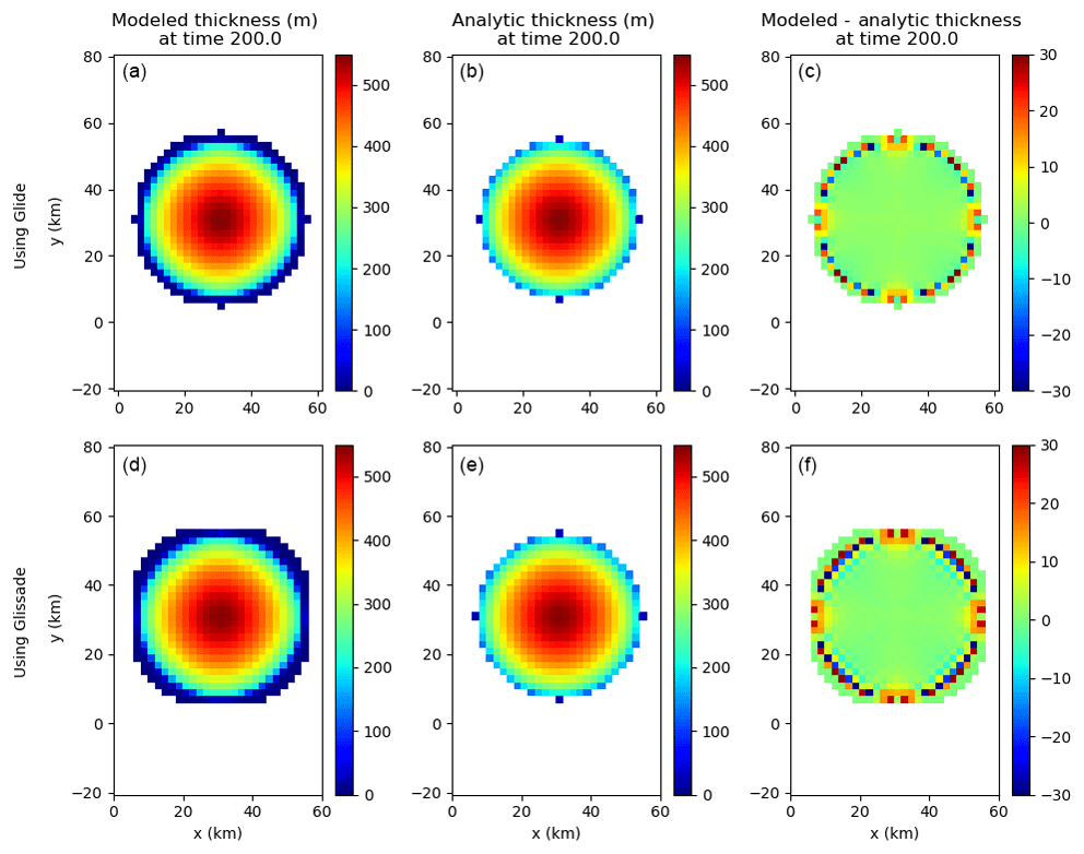
Figure 1Results from the Halfar dome test using SIA solvers from Glide (a, b, c) and Glissade (d, e, f). (a, d) Modeled ice thickness. (b, e) Analytic ice thickness. (c, f) Difference between modeled and analytic thickness.
The bottom panels of Fig. 1 show Halfar results for the Glissade SIA solver described in Sect. 3.1.2, with the same grid and initial conditions and a time step of 1 year (Glissade's explicit transport solver requires a shorter time step than Glide for numerical stability). The errors are larger than for Glide; the rms error is 9.06 m and the maximum error is 34.2 m. Since Glissade's SIA velocity solutions are very similar to Glide's for a given ice sheet geometry, the larger errors can be attributed to the explicit transport solver (Sect. 3.3), which is less accurate for this problem than Glide's implicit diffusion-based solver.
4.2 ISMIP-HOM tests
ISMIP-HOM, described by Pattyn et al. (2008), consists of six experiments, labeled A through F, for higher-order velocity solvers. CISM supports all six experiments, and here we show results for experiments A and C. These two tests are particularly useful for benchmarking higher-order models, since they gauge the accuracy of simulated 3-D flow over a bed with large- and small-scale variations in basal topography and friction.
Experiment A is a test for ice flow over a bumpy bed. The domain is doubly periodic, and the bed topography is sinusoidal in both the x and y directions, with an amplitude of 500 m and wavelength L=5, 10, 20, 40, 80, or 160 km. The mean ice thickness is 1000 m, and the surface slopes smoothly downward from left to right. The velocity field is diagnosed from this geometry given a no-slip basal boundary condition. Figure 2 shows the surface ice speed as a function of x along the bump at , computed using Glissade's BP solver. For L=10 km or more, the solution agrees well with the mean from the Stokes models in Pattyn et al. (2008). At L=5 km, the amplitude is too large (as is typical of BP models), but the magnitude is close to the Stokes solution.
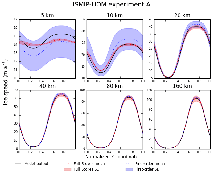
Figure 2Results for ISMIP-HOM experiment A (ice flow over a bumpy bed). Each plot shows the surface ice speed across the bump at for a different length scale L. The solid black line shows output from Glissade's BP velocity solver; the dotted red and blue lines show output from full Stokes and first-order (i.e., higher-order) models, respectively, in Pattyn et al. (2008), and the red and blue shaded regions show the corresponding standard deviations.
Figure 3 shows test A results using Glissade's DIVA solver (cf. Fig. 1 in Goldberg, 2011, which shows similar results from a depth-integrated flowline solver). The DIVA solution is much less accurate than the BP solution; the modeled ice speed is greater than for the Stokes solution, with the relative error increasing as L decreases. These errors are expected, since a bumpy, frozen bed implies that the horizontal velocity gradients are not well approximated (as DIVA assumes) by their vertical averages. The DIVA solution is more accurate, however, than the L1L2 scheme implemented by Perego et al. (2012). The latter scheme does a 2-D matrix solve for the basal velocity and then integrates upward, reducing to the very inaccurate SIA when the basal velocity is zero. DIVA, by solving for the 2-D mean velocity instead of the basal velocity, is more accurate than the SIA.
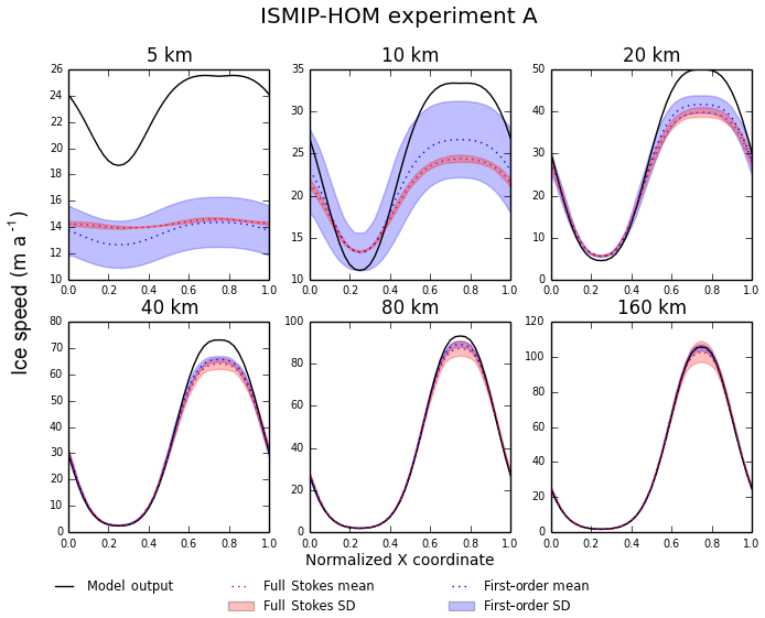
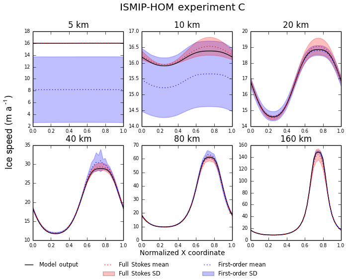
Figure 4Results for ISMIP-HOM experiment C (ice flow over a bed with variable basal friction). Each plot shows the surface ice speed across the bump at for a different length scale L. The solid black line shows output from Glissade's BP velocity solver; the dotted red and blue lines show output from Stokes and first-order models, respectively, in Pattyn et al. (2008), and the red and blue shaded regions show the corresponding standard deviations.
Experiment C is a test for flow over a bed with variable friction. The ice surface and mean thickness are as in experiment A, but the bed is flat, with sinusoidal variations in the basal friction parameter β. Figure 4 shows the surface speed at for each of six wavelengths using the BP solver, and Fig. 5 shows the surface speed using the DIVA solver (cf. Fig. 2 from the depth-integrated flowline solver in Goldberg, 2011). For both BP and DIVA, the CISM results are similar to the Stokes results at all wavelengths. There is a modest difference between BP and DIVA at L=5 km, where the DIVA velocity has a small variation across the domain, whereas the BP and Stokes velocities are nearly uniform.
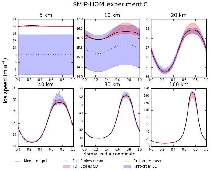
Figure 5Same as Fig. 4, except that the solid black line shows output from Glissade's DIVA velocity solver.
For both experiments A and C, the Glissade BP results are nearly identical to those shown by Tezaur et al. (2015), who used similar finite-element methods to assemble and solve the BP equations.
4.3 Stream tests
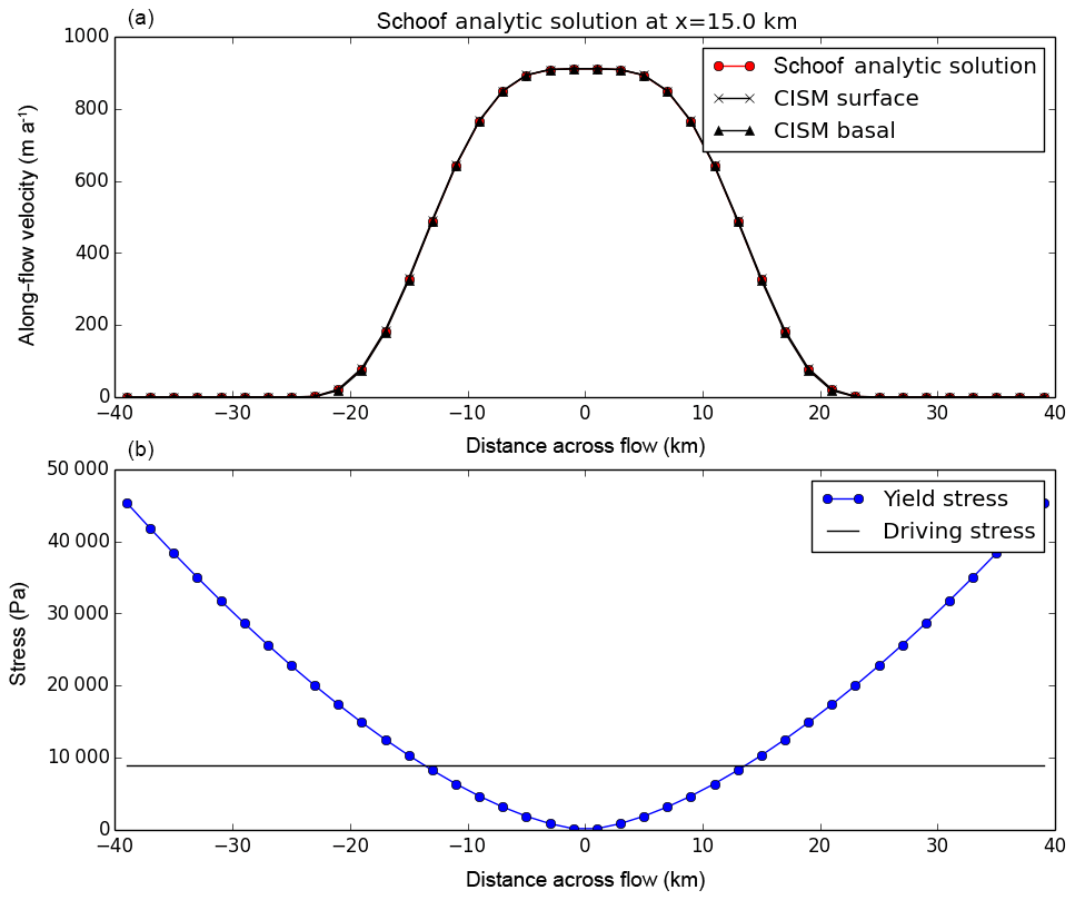
CISM's stream tests simulate flow over an idealized ice stream underlain by subglacial till with a specified yield stress distribution. For the two yield stress distributions specified in this test case, analytical solutions are available from Raymond (2000) and Schoof (2006). For the Raymond test case, the yield stress is given within the ice stream by a uniform value of 5.2 kPa (below the gravitational driving stress of about 10 kPa), and outside the ice stream by a uniform value of 70 kPa (much larger than the driving stress). That is, the yield stress distribution is approximated by a step function. For the Schoof test case, the yield stress across the ice stream varies continuously between about 45 kPa and 0. In both cases, the basal properties and resulting velocity solutions vary in the across-flow direction only and are symmetric about the ice stream centerline.
Figures 6 and 7 compare model results to the analytic Raymond and Schoof solutions, respectively. CISM is run using the BP velocity solver at a grid resolution of 2 km. (DIVA results, not shown, are nearly identical.) The top panels show across-flow velocity profiles, and the bottom panels show the prescribed yield stress and driving stress. In both cases, there is excellent agreement between the modeled and analytic solutions. For the Raymond test, this excellent agreement requires a modified assembly procedure for basal friction terms, as described in Sect. A2, to resolve the step change in yield stress. With the standard finite-element procedure, there is some smoothing of the friction parameter β over neighboring vertices, and the results at a given grid resolution are less accurate. For the Schoof test with a smooth transition in yield stress, either assembly procedure works well.

Figure 6Results from the Raymond stream test using Glissade's BP velocity solver. (a) Across-flow surface and basal velocity (m yr−1) at x=15 km compared to the analytic solution. At most points, the analytic and simulated solutions are indistinguishable. (b) Prescribed yield stress and gravitational driving stress (Pa).
4.4 Shelf tests
CISM includes three shelf tests:
-
The first is a confined-shelf test based on tests 3 and 4 from the Ice Shelf Model Intercomparison exercise (Rommelaere, 1996). This test simulates the flow of a 500 m thick ice shelf within a rectangular embayment that is confined on three sides. Figure 8 shows the 2-D ice speed using Glissade's SSA solver (Sect. 3.1.3) on a 5 km mesh. As expected, the solution is nearly identical to those obtained with the DIVA and BP solvers (not shown). No benchmark is available, but the Glissade solutions are similar to the first-order (BP) solutions found by Perego et al. (2012) and Tezaur et al. (2015) for the same test.
-
The second is a circular-shelf test that simulates the radially symmetric flow of a 1000 m thick ice shelf that is pinned at one point in the center. The SSA solution (not shown) is similar but not identical to the DIVA and BP solutions, since the latter allow vertical shear above the pinning point.
-
The third test simulates the flow of the Ross Ice Shelf in Antarctica under idealized conditions (e.g., a spatially uniform flow-rate factor), as described by MacAyeal et al. (1996). Figure 9, which is based on Figs. 1 and 2 of MacAyeal et al. (1996), shows the ice speed computed by Glissade's SSA solver on the 6.8 km finite-difference grid used in that paper, compared to observed ice speeds. The model velocities agree well with the published velocities from the finite-element model in Fig. 3a of MacAyeal et al. (1996) and, like the published values, tend to be biased fast compared to observations. As noted by MacAyeal et al. (1996), the model–data agreement could be improved by allowing the flow-rate factor to vary spatially. Results from the DIVA and BP solvers (not shown) are nearly identical.
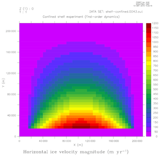
Figure 8Ice speed (m yr−1) for the confined-shelf test (based on tests 3 and 4 from the Ice Shelf Model Intercomparison exercise of Rommelaere, 1996) using Glissade's SSA velocity solver. The ice shelf is 500 m thick. The rectangular domain is open to the south and confined on the other three sides.
4.5 Dome test
CISM's dome test has a simple configuration with a parabolic, radially symmetric dome on a flat bed. It is a general-purpose time-dependent problem that can be used to test not just the velocity solver but also the transport and temperature solvers and various physics options. There is no analytic solution, but the test has proven useful for day-to-day testing.
4.6 Build-and-test structure
To facilitate testing, CISM includes a build-and-test structure (BATS) that can automatically build the model and then run a set of regression tests, including the tests discussed above. BATS allows users and developers to quickly generate a set of regression tests for use with the Land Ice Verification and Validation toolkit (LIVVkit; Kennedy et al., 2017). LIVVkit is designed to provide robust and automated numerical verification, software verification, performance validation, and physical validation analyses for ice sheet models. Instructions on using BATS and LIVV with CISM can be found on the LIVV website (https://livvkit.github.io/Docs/, last access: 20 January 2019).
The CISM v2.0 release included the tests described in Sect. 4 but did not support robust multimillennial simulations of whole ice sheets. Recent work, included in CISM v2.1, has made the model more efficient, reliable, and realistic for Greenland ice sheet simulations. These improvements support the use of CISM in CESM2.0 for century- to millennial-scale Greenland simulations under paleoclimate (e.g., Pliocene and Eemian), present-day, and future climate conditions.
Coupled ice sheet–climate simulations can be problematic, because ice sheets require 104 years or longer to equilibrate with a given climate (Vizcaino, 2014), and because climate is never truly constant on these timescales. If the initial ice sheet conditions in a coupled simulation are not consistent with the climate, then the transient adjustment can swamp any climate change signal. One way to minimize the adjustment is to adjust selected model parameters (e.g., basal traction coefficients or bed topography at each grid point) to satisfy an optimization problem, reducing the mismatch between model variables and observations. In this way, one can generate ice sheet thickness and velocity fields consistent with the SMB from a climate model (Perego et al., 2014). The risk of this approach is that the model can be overtuned to present-day conditions that might not hold on long timescales or in different climates. An alternate approach is to spin up the ice sheet to equilibrium under forcing from a climate model: e.g., steady pre-industrial forcing or forcing spliced together from two or more climate time slices (Fyke et al., 2014). Because of climate model biases, however, the spun-up ice thickness and velocity can differ substantially from modern observations.
Here, we take the second approach, spinning up the Greenland ice sheet with surface forcing from the regional climate model RACMO2.3p1 statistically downscaled to 1 km resolution (Noël et al., 2016). Since RACMO2 is run at high resolution, is constrained by reanalysis at model boundaries, and is well validated against observations, its SMB is more realistic than that of a global climate model. RACMO2 provides the SMB only for the region included within its ice sheet mask; outside this region, we prescribe a negative SMB. The ice sheet is initialized with present-day extent and thickness, and then is spun up for 50 000 years (long enough to reach quasi-equilibrium) on a 4 km grid (the standard grid for CESM ice sheet simulations).
We analyze two experiments. The first experiment uses a “no-float” calving scheme, in which floating ice is assumed to calve immediately. A similar configuration was used to initialize CISM for the initMIP-Greenland experiment (Goelzer et al., 2018). The no-float assumption simplifies model setup and analysis, while still simulating ice flow for the vast majority of the Greenland ice sheet. The second experiment uses the eigencalving scheme described in Sect. 3.5, along with the depth-dependent sub-shelf melting scheme of Sect. 3.6. This simulation tests the model's ability to generate robust, stable ice shelves that at least roughly resemble Greenland's present-day ice shelves, including the floating shelf of Petermann Glacier in northern Greenland and two floating termini of the Northeast Greenland Ice Stream (NEGIS): Nioghalvfjerdsbræ (79 North Glacier) and Zachariae Isstrom.
Although the model has been configured to give results that are reasonably realistic, these spin-ups should be viewed primarily as a demonstration of CISM capabilities, not as scientifically validated simulations. For example, model tuning has likely compensated for biases in the forcing data. Generally speaking, model parameters should always be tested and reviewed depending on the science application.
5.1 Simulation without ice shelves
The simulation without floating ice shelves is configured as follows:
-
The model is initialized with present-day ice sheet geometry. The ice thickness and bed topography are based on the mass-conserving-bed method of Morlighem et al. (2011, 2014).
-
The SMB forcing over the Greenland ice sheet is a 1958–2015 climatology from RACMO2.3p1 (Noël et al., 2016). For ice-free regions where RACMO2 does not compute an SMB, the SMB is arbitrarily set to −4 m yr−1, thus limiting deviations from present-day ice extent. The surface temperature is from the 20th century RACMO2 climatology of Ettema et al. (2009).
-
The basal geothermal heat flux is prescribed from Shapiro and Ritzwoller (2004).
-
Where the SMB is negative, the initial temperature profile in each column is linear, with at the surface and at the bed. Where the SMB is positive, the temperature is initialized to an analytic profile based on a balance between vertical conduction and cold advection (Cuffey and Paterson, 2010, Sect. 9.5.1). This profile is relatively cold in the upper part of the ice sheet.
-
The 3-D velocity field is computed at 11 vertical levels using the DIVA solver described in Sect. 3.1.4. Thickness and tracer evolution are given by the incremental remapping scheme of Sect. 3.3, with a time step dt=0.2 years.
-
The basal friction coefficient β is computed at each vertex using a pseudo-plastic sliding law as described in Sect. 3.4. This scheme has several parameters that can be tuned to reduce effective pressure and increase sliding in warm, low-elevation regions. Parameter values, mostly following Aschwanden et al. (2016), are q=0.5 and u0=100 m yr−1, with ϕ decreasing from 40 to 5∘ as the bed elevation decreases from 700 to −700 m.
-
Effective pressure is a function of basal water depth as computed by the local till model described in Sect. 3.4 with till parameters from Bueler and van Pelt (2015). In particular, Wmax=2 m, Cd=1 mm yr−1, and δ=0.02.
-
Floating ice calves immediately, and marine cliff heights are limited as described in Sect. 3.5.
-
Some of the model physics is constrained to make the simulation more robust. The surface gradients and in the gravitational driving stress are limited to a magnitude of 0.10 to prevent unrealistically large ice speeds in coastal regions with steep topography, and β is held to a minimum of 100 Pa m−1 yr for grounded ice to prevent very fast sliding.
After 50 000 model years, the ice sheet extent and volume have equilibrated to 1.63×10⁶ km2 and 2.97×10⁶ km3, respectively, in close agreement with values of 1.67×10⁶ km2 and 2.95×10⁶ km3 in the observational data set (Morlighem et al., 2014). The close agreement between observed and modeled extent and volume depends, in part, on the negative SMB applied outside the RACMO2 ice sheet mask to inhibit ice advance. We checked for equilibrium by comparing thickness snapshots at 500-year intervals near the end of the run. Thickness variations over the last 1000 years (not shown) are less than 50 m everywhere on the ice sheet.
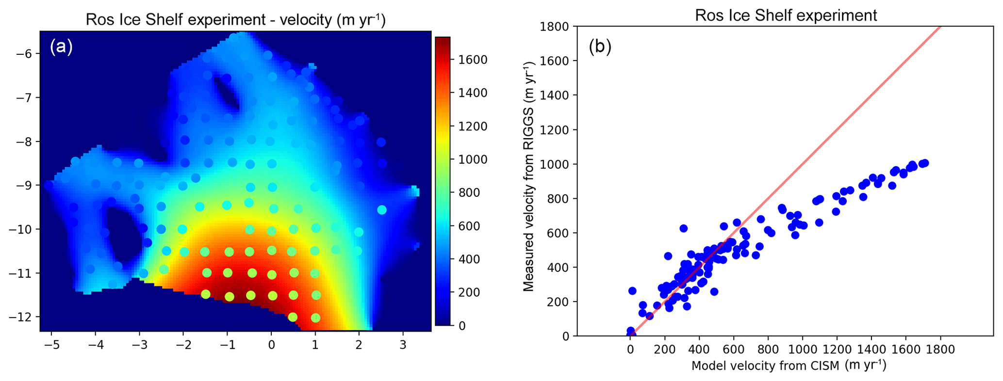
Figure 9Results of the Ross Ice Shelf test described by MacAyeal et al. (1996), computed using Glissade's SSA solver. Panel (a), based on Fig. 1 of MacAyeal et al. (1996), shows the vertically uniform ice speed (m yr−1). The circles indicate locations where ice speed was measured by the Ross Ice Shelf Geophysical and Glaciological Survey (RIGGS); measured speeds are shaded with the same color scale as the observations. Axis coordinates match the coordinates in MacAyeal et al. (1996). Panel (b), based on Fig. 2 of MacAyeal et al. (1996), compares simulated to measured ice speeds at the RIGGS locations.
Figure 10 shows the surface ice speed at the end of the run, compared to observations. In most of the ice sheet, the simulated ice flow is in good agreement with observations. The model captures slow-flowing regions in the interior where the bed is frozen, as well as fast-flowing outlet glaciers along the margins. A major shortcoming of the simulation is its failure to capture NEGIS, which in reality extends far into the northeast interior but is simulated to be slower, shorter, and more diffuse. Aschwanden et al. (2016), who ran PISM using the pseudo-plastic basal sliding scheme adopted by CISM, obtained similar results. While capturing complex outlet glacier flow, both models have a poor representation of NEGIS, possibly due to a missing geothermal heat source or simplified subglacial hydrology.

Figure 10Surface ice speed (m yr−1, log scale) for the Greenland ice sheet. (a) Observed speed (Joughin et al., 2010). (b) Simulated speed at the end of a 50 kyr Greenland spin-up without floating ice shelves. The gray background shows ice-free regions. Figures 10–17 were created using the NCAR Command Language (2017).
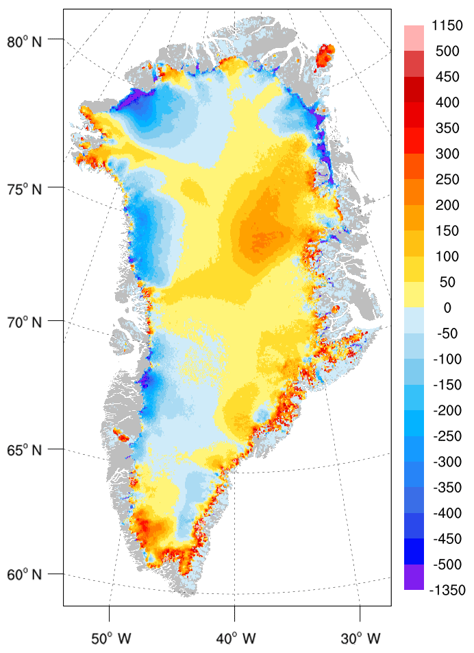
Figure 11Difference (m) between (1) simulated ice thickness at the end of a 50 kyr Greenland spin-up without ice shelves and (2) observed thickness from Morlighem et al. (2014). The observed thickness is the model initial condition. The gray background shows regions that are ice-free at both the beginning and end of the simulation.
Figure 11 shows the difference between the final ice thickness and the observed initial thickness. In most of the interior, the thickness errors are ∼100 m or less, with the main exception being the upper part of NEGIS, where slow flow correlates with a positive thickness bias of ∼200 m. Errors are larger along the margins, with positive biases of up to ∼500 m in the southeast, where accumulation is large, and negative biases of up to ∼500 m in the north and northwest, where accumulation is lower and there is significant ablation at the margins. Low thicknesses along the coast could result from excessive marginal ablation in the SMB data set, insufficient basal friction, or a combination. High thickness in the southeast could be attributed to positive accumulation biases in the data set or too-slow flow in outlet glaciers, among other factors.
Figure 12 illustrates the basal water state. The ice sheet is shaded to indicate three regions: a frozen central region (extending to parts of the northern and eastern margins) with basal water depth W=0; thawed coastal regions, especially along the western margin and in major outlet glacier basins where W is capped at 2 m; and intermediate regions where m. The color scheme in Fig. 12 was chosen for comparison to Fig. 11 from MacGregor et al. (2015), who presented a synthesis of Greenland's basal state from observations and models. The agreement is generally excellent (though the two results are not fully independent, since models similar to CISM were part of the synthesis). The largest area of discrepancy is the upstream part of NEGIS, which is thawed or uncertain in the synthesis but frozen in the model.
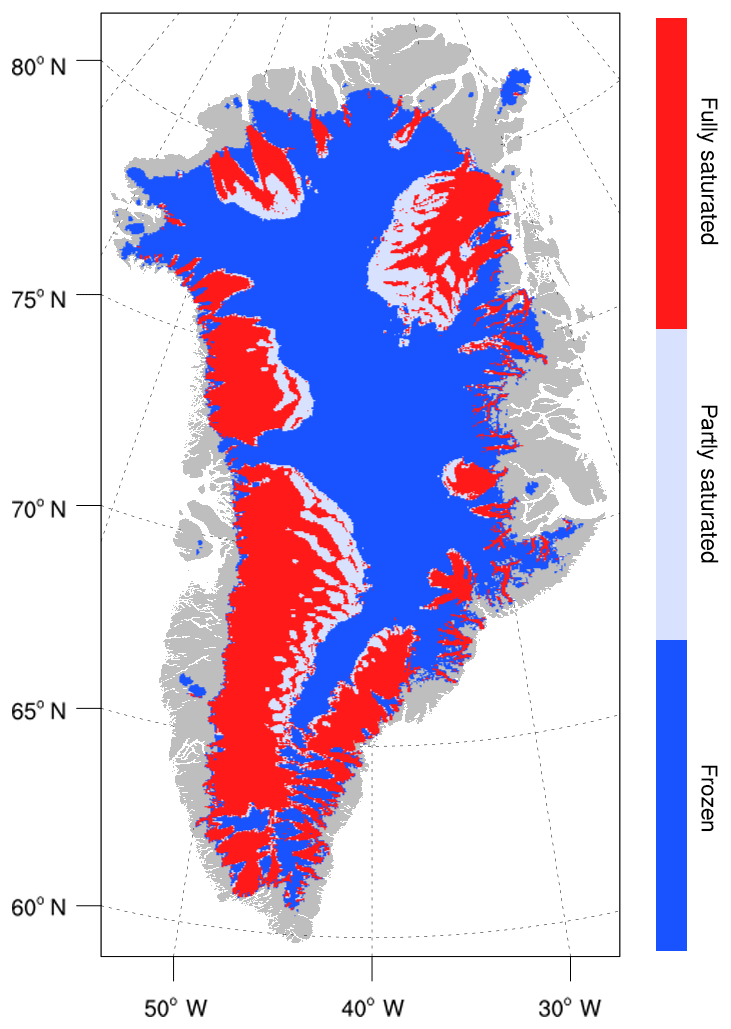
Figure 12Basal water state at the end of a 50 kyr Greenland spin-up. Red: fully saturated bed with basal water depth W capped at the upper limit of 2 m. Light blue: partly saturated bed with m. Dark blue: frozen bed with W=0. The color scale is based on Fig. 11 of MacGregor et al. (2015). The gray background shows ice-free regions.
The intermediate regions in Fig. 12 have striped patterns with century-scale temporal variability, consistent with the band-like patterns in driving and basal shear stresses found by Sergienko et al. (2014) in regions with rapid basal sliding. Sergienko et al. (2014) attributed these patterns to instabilities related to subglacial water. A more detailed investigation would be needed to determine how robust these features are in the model, and to what extent they are real features as opposed to numerical artifacts.
As shown by Schoof and Hindmarsh (2010), depth-integrated approximations like DIVA are computationally much cheaper than BP while incurring only a small loss of accuracy, mainly in slow-sliding regions. However, their analysis did not consider the effects of vertically varying temperature. In CISM simulations of real ice sheets, the depth-integrated viscosity depends on the vertical temperature profile (see Eqs. 2 and 24), with dynamic effects that are not included in idealized problems with a uniform temperature or flow factor. To assess possible errors associated with the DIVA solver (taking BP to be “truth”), we ran CISM for 10 000 years using the BP solver, with settings and forcing otherwise identical to the DIVA run. After 10 kyr, the ice sheet area and volume are 1.635×10⁶ km2 and 2.991×10⁶ km3, respectively, for the BP run, compared to 1.634×10⁶ km2 and 2.993×10⁶ km3 for DIVA. Figures 13 and 14 show differences in thickness and surface ice speed, respectively, between the two runs. In the vast majority of the ice sheet, thickness differences are less than 50 m, and velocity differences are less than 20 m yr−1. In several outlet glaciers, however – notably Humboldt Glacier in the northwest – thickness differences exceed 100 m, and velocity differences are greater than 100 m yr−1. These differences might merit further study. Some, although not all, of the larger differences can be attributed to transient behavior. For example, Humboldt Glacier is not fully equilibrated at 10 kyr, and the two simulations could capture the glacier in different phases.
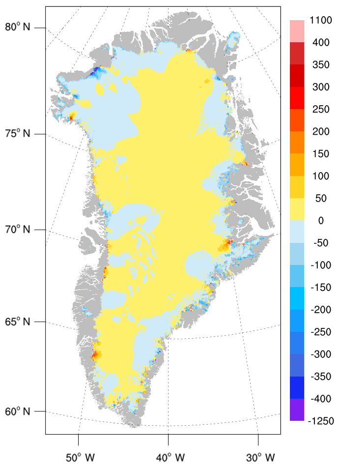
Figure 13Difference (m) in simulated ice thickness after 10 kyr between (1) a run using the BP velocity solver and (2) a run using the DIVA velocity solver and otherwise configured identically. The gray background shows regions that are ice-free in both simulations.

Figure 14Difference (m yr−1) in simulated ice speed after 10 kyr between (1) a run using the BP velocity solver and (2) a run using the DIVA velocity solver and otherwise configured identically. The gray background shows regions that are ice-free in both simulations.
Table 3Computational performance on NCAR's Cheyenne supercomputer for various simulations: DIVA vs. BP solvers, with and without floating ice shelves, and 144 vs. 288 processor cores.
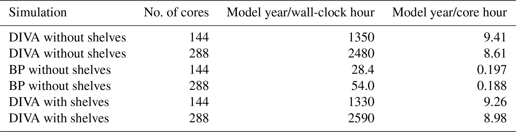
Table 3 shows the cost of these runs on 144 and 288 cores of NCAR's Cheyenne supercomputer. On 144 cores, the DIVA run without ice shelves completes 1350 model years per wall-clock hour or 9.41 model years per core hour. Running on 288 cores, the throughput increases to 2480 model years per wall-clock hour, at slightly reduced efficiency of 8.61 model years per core hour. With the BP solver and an otherwise identical configuration (including 11 vertical velocity levels), the throughput decreases by nearly a factor of 50. Table 3 also shows the cost of DIVA runs with ice shelves, which are described next. Although we have found that solver convergence can be slower when floating ice is present, the runs presented here have a similar cost with or without ice shelves.
5.2 Simulation with ice shelves
The simulation with ice shelves is configured like the no-shelf simulation but with these differences:
-
No-float calving is replaced by the eigencalving scheme of Sect. 3.5, with kτ=0.0025 m yr−1 Pa−1 and w2=25. These parameters give a low calving rate for along-flow tensile stresses and a much higher rate for across-flow stresses.
-
Beneath floating ice, we apply the depth-dependent melt rate of Sect. 3.6, with a basal mass balance b=0 at m. The freezing rate is 3 m yr−1 above m, with a linear ramp between −200 and −100 m. The melt rate is 100 m yr−1 below m, with a linear ramp between −200 m and −500 m. The scale for reducing melting in shallow cavities is H0=20 m.
Choi et al. (2017) used a similar combination of stress-based calving and depth-dependent sub-shelf melting in ISSM to simulate glacier evolution in the NEGIS region. For the CISM simulations, calving and melting parameters were tuned to improve agreement with Greenland's observed ice shelves (or lack thereof). For example, higher values of kτ were found to remove existing ice shelves in northern Greenland. With the chosen value of kτ, lower values of w2 are insufficient to calve long, unrealistic ice tongues along the southeast coast. Similarly, sub-shelf freezing is needed near the surface to prevent substantial calving-front retreat for the Petermann and 79 North glaciers. While near-surface freezing is physically plausible, basal freezing in the simulation might be compensating for a negative SMB bias (Noël et al., 2018) or excessive calving. A maximum melt rate of 100 m yr−1 exceeds inferred melt rates of ∼30 m yr−1 near the grounding line (GL) of Petermann Glacier (Cai et al., 2017), but smaller rates in the model permit unrealistic GL advance. Simulated GL locations could differ, however, if the model were run at different resolution or with a grounding-line parameterization (Gladstone et al., 2010; Leguy et al., 2014).
By the end of a 50 000-year simulation with ice shelves, the total ice area and volume reach equilibrium values of 1.67×10⁶ and 3.08×10⁶ km2, respectively. The area agrees closely with the observational data set, but the volume is high by about 4 %. The floating area more than doubles compared to observations, from 3.7×10³ to 9.2×10³ km2. The additional floating ice is contained in many small shelves along the coasts.
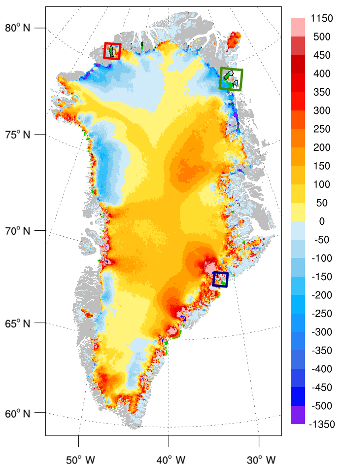
Figure 15Difference (m) between (1) simulated ice thickness at the end of a 50 kyr Greenland spin-up with ice shelves and (2) observed thickness from Morlighem et al. (2014). The observed thickness is the model initial condition. The thickness difference is shown for grounded ice only. Regions shaded light green are floating at the end of the simulation, and black contours enclose regions that are floating in observations. The three boxes indicate floating regions highlighted in Fig. 17: Petermann Glacier (red), 79 North Glacier and Zachariae Isstrom (dark green), and Kangerlussuaq Glacier (dark blue). The gray background shows regions that are ice-free at both the beginning and end of the simulation.
Figure 15 shows (for grounded ice) the thickness difference between the simulation and observations. Simulated floating ice is shaded light green, and observed floating ice is enclosed by black contours. The pattern of thickness errors is generally similar to the run without ice shelves (Fig. 11), with positive biases in the northeast interior and along the southeast coast, and negative biases along the northern and northwest margins. The run with shelves, however, has additional positive biases in east central and west central Greenland, upstream of large outlet glaciers such as Jakobshavn in the west and Helheim and Kangerlussuaq in the southeast. The basins that have thickened relative to the no-shelf simulation generally have ice shelves at their termini, where no shelves exist in reality. Although these shelves are small, they appear to provide buttressing that leads to thickening upstream. Figure 16 shows the difference in surface ice speed between the simulations with and without ice shelves. Differences are largest in outlet glaciers with unrealistic floating termini. The general pattern is of faster speeds near glacier termini in the run with shelves (where ice can be much thicker than in the no-shelf simulation), with slower speeds upstream.
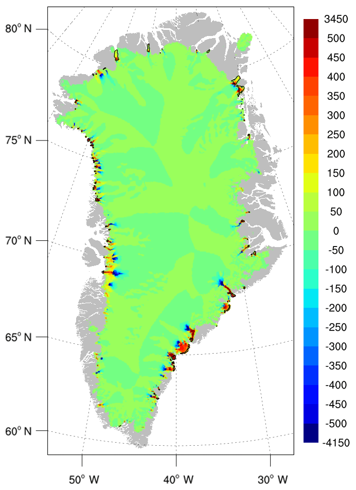
Figure 16Difference (m yr−1) in simulated surface ice speed at the end of 50 kyr Greenland spin-up runs with and without ice shelves. Black contours enclose regions that are floating in the run with ice shelves. The gray background shows regions that are ice-free in both simulations.
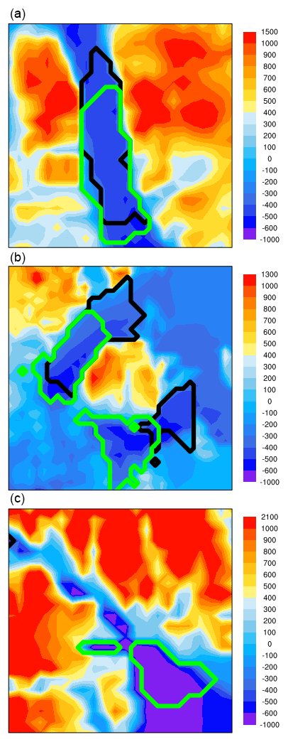
Figure 17Close-ups of three regions with floating ice at the end of a 50 kyr Greenland spin-up with ice shelves: Petermann Glacier (a), 79 North Glacier and Zachariae Isstrom (b), and Kangerlussuaq Glacier (c). These regions are enclosed by boxes in Fig. 15. The shaded color shows the bed topography (m). Black and green contours enclose regions that are floating at the start and end of the simulation, respectively. Calving fronts are located at the north, northeast, and southeast shelf boundaries, respectively, from top to bottom; grounding lines are located at the south, southwest, and northwest shelf boundaries, respectively.
Figure 17 shows closeups of three regions enclosed by boxes in Fig. 15. These regions illustrate floating ice simulated in the vicinity of Petermann Glacier in the northwest, 79 North Glacier/Zachariae Isstrom in the northeast, and Kangerlussuaq Glacier in the southeast. The Petermann simulation (Fig. 17a) is the most realistic, with modest retreat of both the grounding line and calving front, and a total area similar to observations. As mentioned above, however, both the CF and GL locations are sensitive to model parameters. The 79 North Glacier ice shelf (upper left of Fig. 17b) shows modest GL retreat with somewhat larger CF retreat. The simulated Zachariae shelf (lower right of Fig. 17b) substantially retreats; we found no combination of calving and basal melting/freezing parameters that maintains Zachariae in its observed location. Figure 17c, showing Kangerlussuaq Glacier, illustrates the model's tendency to grow unobserved shelves. While there is little floating ice in this region in reality, there is a moderate-sized simulated shelf at the fjord mouth, buttressing the glacier upstream.
These results demonstrate a modeling challenge for Greenland: how to simulate existing ice shelves in northern Greenland without permitting unrealistic shelves in other regions. An eigencalving parameterization, suitably tuned, can prevent shelves from extending into the open ocean, but in enclosed bays there are unrealistic shelves with non-negligible dynamic effects. We were unable to eliminate the unobserved shelves in CISM without also removing observed shelves. This result suggests that important calving or melting mechanisms could be missing in the model. For example, Bassis and Ma (2015) suggested that basal melting, which is spatially variable, is a major driver of crevassing and calving. Lacking ocean forcing, the model does not simulate spatially dependent basal melt rates.
Despite these biases, the results show that CISM is capable of simulating ice velocities broadly consistent with observations for both slow-flowing and fast-flowing parts of the Greenland ice sheet, with reasonable computational costs for multimillennial simulations with a higher-order Stokes approximation.
We have described CISM v2.1, which includes many innovations to support robust, accurate, and efficient ice sheet simulations in both idealized and real-world applications. The model incorporates a hierarchy of Stokes approximations, including SIA, SSA, depth-integrated higher-order, and 3-D higher-order. To solve the large elliptic systems associated with membrane stresses, CISM has an efficient native Fortran preconditioned conjugate gradient solver, along with links to third-party solver libraries (Trilinos and SLAP). CISM also adds test cases for higher-order models, including ISMIP-HOM and various shelf and stream cases. For each velocity solver and test case, we have verified that CISM solutions are consistent with community benchmarks. That is, the solutions are as accurate as expected given the simplifications in the various approximations.
CISM's structured rectangular grid has limitations; in particular, the grid cannot be refined selectively near grounding lines and other regions requiring high resolution. On the other hand, the structured grid lends itself to straightforward algorithm development, debugging, creation of forcing data sets, and analysis of results. CISM runs efficiently on a 4 km Greenland grid, with throughput of ∼2000 model years per wall-clock hour on NCAR's Cheyenne supercomputer using the depth-integrated higher-order solver. Performance improvements might be needed, however, to support whole-ice-sheet simulations on grids as fine as 1 or 2 km.
CISM has participated in the initMIP-Greenland experiments (Goelzer et al., 2018) for model initialization. When spun up for 50 kyr with modern climate forcing and without floating ice, CISM gives a steady-state simulation in good agreement with the observed ice extent, volume, and velocity structure of the Greenland ice sheet. The quality of the simulation can be attributed, in part, to a higher-order solver that simulates a realistic stress state in fast outlet glaciers, along with a pseudo-plastic basal sliding law that enhances sliding on thawed beds at low elevation. The simulation also benefits from an accurate SMB (from the regional climate model RACMO2), adjusted to inhibit ice sheet advance beyond modern boundaries. When floating ice is allowed, CISM can maintain ice shelves that resemble observed shelves in northern Greenland, but the model also simulates many small shelves that do not exist in reality.
CISM can be used for both stand-alone and coupled ice sheet simulations. CISM v2.1 is the dynamic ice sheet component of CESM2.0, released in June 2018. Compared to earlier CESM versions, CESM2.0 has more sophisticated ice sheet dynamics and physics (as described here), along with interactive coupling capabilities. These improvements will support increasingly realistic simulations of coupled ice sheet evolution.
Source code for CISM v2.1 can be obtained by downloading a released version from https://cism.github.io/download.html (Hoffman et al., 2019) or by cloning the code from the public git repository at https://github.com/CISM/cism (last access: 20 January 2019). The CISM2.1 documentation, which includes detailed instructions for downloading and building the code, can be found at https://cism.github.io/documentation.html (last access: 20 January 2019).
Following the release of CESM2.0 in June 2018, new CISM development was moved to the Earth System Modeling Community Portal (ESCOMP). The latest code is available on the public git repository at https://github.com/escomp/cism (Sacks and Lipscomb, 2019). Current documentation for CISM and for the land-ice implementation in CESM can be found at http://www.cesm.ucar.edu/models/cesm2/land-ice/ (last access: 20 January 2019). New developers are welcome.
Here, we describe the assembly of the terms in Eq. (9) into a global matrix A and vector b. The four terms in Eq. (9) describe internal ice stresses, basal friction, lateral pressure, and the gravitational driving force, respectively. We begin with the internal stress term, which is the most complex.
A1 Internal ice stresses
The first term on the LHS of each component of Eq. (9) can be rewritten in terms of velocity components:
where brackets denote row vectors and braces denote column vectors. Glissade evaluates Eq. (A1) for each active element. Hexahedral elements have eight nodes, with u and v to be determined at each active node. Inserting the velocity expressions (Eq. 6) into Eq. (A1), we obtain
Each row or column vector has eight terms, one for each node of the element. These terms can be evaluated to form a set of four 8×8 element matrices, denoted as Kuu, Kuv, Kvu, and Kvv. Each row of an element matrix is associated with u or v at a given node. The columns in this row contain terms linking the node to u or v at the other nodes of the same element (with the diagonal term linking the node to itself).
In the x component of Eq. (A2), the terms that multiply uj are given by
Letting i and j range from 1 to 8, Eq. (A3) gives the 64 terms of the 8×8 element matrix Kuu, which links the u value at each node to the u values at all eight nodes. Similarly, the 64 terms of element matrix Kuv, which links u at each node to v at each of the eight nodes, are given by
Likewise, two 8×8 matrices are associated with the y component of Eq. (A2). The terms of Kvu are
and the terms of Kvv are
Because of the symmetry of the underlying PDEs, Kuu and Kvv are symmetric, and . The terms containing z (i.e., the vertical shear stresses) appear only in Kuu and Kvv, whereas the terms containing x and y (i.e., the membrane stresses) appear in all four element matrices.
In the weak form of the equations, each of the 64 coefficients in each element matrix must be integrated over the element. (Since φ varies over the element, the integrands in Eqs. A3–A6 have a different value at each point.) The integrals can be computed exactly by evaluating the integrand at each of eight quadrature points and summing over quadrature points.
We now specify the form of the basis functions and transform these functions to the geometry of the element (which is irregular in the vertical direction because of the sigma coordinate). We can then evaluate the basis function derivatives at quadrature points. Glissade uses trilinear basis functions defined on a reference cube. This cube is centered at the origin in local reference coordinates ). The eight nodes of the reference cube are located at . By convention, nodes 1–4 are the nodes of the lower face, proceeding counterclockwise from the southwest corner . Nodes 5–8 are the nodes of the upper face, also moving counterclockwise from the southwest corner. Thus, we have
For each n, we have φn=1 at node n, with φn=0 at the other nodes.
The integrands in Eqs. (A3)–(A6) are written in terms of real Cartesian coordinates rather than reference coordinates . Spatial derivatives in real coordinates are related to derivatives in reference coordinates by
where [J] is the Jacobian of the transformation between coordinate systems. Given the finite-element expansion,
along with the spatial derivatives of φ at (which are easily derived from Eq. A7), we can compute as
We then invert Eq. (A8) to obtain the basis function derivatives in terms of :
The LHS of Eq. (A11) contains the spatial derivatives needed to evaluate Eqs. (A3)–(A6).
Equations (A3)–(A6) also contain the viscosity η, which is computed at each quadrature point. In the BP approximation, η is given by Eq. (2); it is a function of the flow factor A and the effective strain rate defined by Eq. (3). We approximate A by its value at the element center. The (squared) effective strain rate is evaluated at each quadrature point by summing over strain-rate components. The x components are given by
and similarly for the y and z components. The nodal velocities in Eq. (A12) are values from the previous iteration.
We now have the information needed to compute the integrands (A3)–(A6) at quadrature points. To integrate over a hexahedron, we take a weighted sum of the values at each of eight quadrature points. These points are located at reference coordinates . To evaluate an integral of the form
over element volume Ω, we compute the sum over quadrature points
where is the determinant of the Jacobian (Eq. A10). For this choice of quadrature points, each point has a weight wp=1.
The terms of the element matrices , and Kvv are then inserted into the corresponding global matrices , and Avv. This is mostly a matter of bookkeeping. For example, the first row of Kuu corresponds to a particular node of element (specifically, the node with indices , given the convention for numbering nodes within elements). This row corresponds to a row of the global matrix Auu, and each of the eight terms in the row of Kuu is associated with a column of Auu. Glissade determines the correct column and adds the Kuu term to the corresponding term in Auu. This process proceeds until the code has looped over all the active elements and filled the global matrices.
If written in full, each global matrix would have as many rows and columns as there are active nodes. These matrices, however, are sparse, with a maximum of 27 nonzero terms per row (corresponding to a node and its 26 nearest neighbors in a hexahedral lattice). Glissade therefore assembles and stores arrays of dimension , where nx, ny, and nz are the grid dimensions. The 27 terms of the first array dimension are arranged according to a geometric convention. For example, suppose we are filling columns for the matrix row corresponding to node . Then, by convention, index 1 refers to the node with coordinates , index 14 refers to the node itself (i.e., the diagonal term of the row), and index 27 refers to the node at (and similarly for the other indices). After assembly, these arrays can be converted to the form required by a particular linear solver.
The remaining assembly consists of evaluating the other terms in Eq. (9) (i.e., the basal and lateral boundary conditions and the gravitational forcing) and implementing Dirichlet boundary conditions, if applicable. We consider these in turn.
A2 Basal boundary conditions
The basal boundary terms in Eq. (9) are
The basal face of each cell is a rectangle. To integrate over a rectangle, we sum over four quadrature points lying at in a reference square with center (0,0) and vertices . This reference square is the 2-D analog of the reference cube discussed above. We define four bilinear basis functions on the square (cf. Eq. A7):
Given these basis functions and their spatial derivatives, we can compute the Jacobian for the transformation between the reference square and the rectangular cell face using the 2-D versions of Eqs. (A10) and (A11):
The integrand at a quadrature point has the form βφiφj, where the second φ term arises from the finite-element expansion of u at a quadrature point:
We determine β at quadrature points from the values at cell vertices:
The integral over a cell is then computed as a sum over quadrature points:
where wp=1 for each point. This procedure yields a 4×4 matrix describing the connections between each vertex and its neighbors in the cell. Since the x term in Eq. (A15) contains u but not v, and the y term contains v but not u, we form 2-D matrices Kuu and Kvv, but not Kuv and Kvu. Each term of Kuu is then inserted into the global matrix Auu, and similarly for Kvv into Avv.
This assembly method tends to smooth the β field. If it is desired to resolve sharp discontinuities in β, as in the stream test problem of Sect. 4.3, Glissade supports a local assembly method in which the basal friction at a particular vertex depends on the value of β at that vertex alone.
A3 Lateral boundary conditions
The lateral boundary terms in Eq. (9) are
Since these terms are independent of u and v, they contribute to the load vectors bu and bv on the right-hand side of Eq. (16). They are integrated over the lateral faces of cells (either grounded or floating) that border the ocean.
The lateral faces bordering the ocean are quadrilaterals that can be mapped to a reference square. The integral over each face is found by summing over four quadrature points. Basis functions are given by Eq. (A16), and the Jacobian of the reference square is found using Eq. (A17). The ice thickness H at each quadrature point is evaluated using
where the Hn are nodal values interpolated from cell centers.
The integrands have the form pφ, where p is the vertically averaged net pressure normal to the ice edge, given by Eq. (13). The integral of the pressure terms over a lateral face is computed as a sum over quadrature points:
where the sign depends on the orientation of the face. The resulting pressure terms are inserted into the load vector (either bu or bv, depending on the orientation) in the rows associated with each of the four nodes of the face.
A4 Gravitational driving stress
The gravitational forcing terms in Eq. (9) are
To compute these terms, we evaluate and at each active vertex, typically using Eq. (14) or its y analog.
The integrals in Eq. (A25) are over 3-D elements. Each hexahedral element is mapped to a reference cube as described above. Given at the vertices of a cell, the surface slope terms at quadrature points are
where the basis functions φ are given by Eq. (A7) and the spatial derivatives are derived from Eqs. (A10) and (A11). The integral of over an element is evaluated as a sum over quadrature points:
and similarly for the term. Glissade inserts these terms into the load vectors bu and bv.
As described above for the assembly of β terms, this method tends to smooth the surface elevation gradient field, averaging neighbor values of and into the driving stress at each vertex. For problems with sharp variations in surface gradients, we have found the solver to be more robust when the driving stress at each vertex depends on and at that vertex alone. Thus, Glissade also supports a local assembly method for the driving stress.
A5 Dirichlet boundary conditions
Once the matrix has been assembled, it may need to be adjusted for Dirichlet boundary conditions (i.e., prescribed velocity values at certain nodes). A common Dirichlet condition is to set at the bed to enforce a no-slip boundary condition. (A no-slip condition can also be enforced by setting the basal traction coefficient β to a large value, but formally this is not a Dirichlet condition.) Also, it may be desirable to set u and v to observed values at certain locations, as in the Ross Ice Shelf test case (Sect. 4.4).
Suppose that at node we have u=uc and v=vc, where uc and vc are prescribed values. Let nr be the row of Auu associated with this node, and let nc range over the columns with nonzero entries in this row. To enforce the Dirichlet condition, we set for all values of nc except nc=nr (the diagonal term); we set . In addition, we set for all nc, since these two matrices do not contain any terms on the diagonal of the full global matrix (i.e., A in Eq. 15). On the right-hand side, we set bu(nr)=uc and bv(nr)=vc. These operations convert the matrix rows associated with node to the equations , which clearly have the desired solutions uc and vc.
A further step is needed to maintain matrix symmetry, as required for the PCG solver. Consider the term Auu(nr,nc), where nc is a column associated with a neighboring node. We have already set , so we need to set to maintain symmetry. The Dirichlet condition is u(nr)=uc. Thus, we can replace bu(nc) with and set without altering the problem. We do this for all the terms in the columns associated with node (i.e., all the terms multiplied by uc or vc in the matrix–vector product). Thus, both the rows and the columns associated with node are filled with zeros, except for the diagonal term, and the full global matrix remains symmetric.
WHL, SFP, and MJH were the primary developers of CISM; WHL led development of the Glissade dycore. KJE, GRL, MP, DMR, WJS, AGS, and PHW contributed to various parts of the code, including parallel infrastructure, performance metrics, links to Trilinos, and links to CESM. JHK, KJE, and ARB integrated CISM verification and validation tests into the LIVVkit package. ARB, SLB, JGF, JHK, GRL, and LV helped set up and analyze Greenland experiments. WHL wrote the paper with contributions from SFP, MJH, and GRL, and with input from all authors.
The authors declare that they have no conflict of interest.
CISM development was supported primarily by the Earth System Modeling program, Office of Biological and Environmental Research (BER) of the US Department of Energy's Office of Science. Additional support was provided by the DOE's Office of Advanced Scientific Computing Research (ASCR), by BER's Regional and Global Climate Modeling Program, and by the National Science Foundation. This material is based upon work supported by the National Center for Atmospheric Research, which is a major facility sponsored by the National Science Foundation under cooperative agreement no. 1852977. Computing resources (https://doi.org/10.5065/D6RX99HX) were provided by the Climate Simulation Laboratory at NCAR's Computational and Information Systems Laboratory, sponsored by the National Science Foundation and other agencies. Lauren J. Vargo was supported by NSF grant ANT-0424589 to the Center for Remote Sensing of Ice Sheets (CReSIS). This paper has been authored by UT-Battelle, LLC, under contract no. DE-AC05-00OR22725 with the US Department of Energy. The United States Government retains and the publisher, by accepting the article for publication, acknowledges that the United States Government retains a non-exclusive, paid-up, irrevocable, worldwide license to publish or reproduce the published form of this paper, or allow others to do so, for United States Government purposes.
We thank Jan Lenaerts and Brice Noël for providing surface forcing data
sets from RACMO2. We are also grateful to Rob Arthern, Xylar Asay-Davis, Andy
Aschwanden, Jeremy Bassis, Jed Brown, Ed Bueler, Steph Cornford, John
Dukowicz, Heiko Goelzer, Dan Goldberg, Jesse Johnson, Eric Larour, Marcus
Löfverström, Dan Martin, Mathieu Morlighem, Sophie Nowicki, Frank Pattyn,
Tony Payne, David Pollard, Hélène Seroussi, Slawek Tulaczyk, Miren
Vizcaíno, and Morgan Whitcomb for helpful discussions. We thank Johannes
Sutter and one anonymous referee for constructive
comments.
Edited by: Philippe Huybrechts
Reviewed by: Johannes Sutter and one anonymous referee
Albrecht, T., Martin, M., Haseloff, M., Winkelmann, R., and Levermann, A.: Parameterization for subgrid-scale motion of ice-shelf calving fronts, The Cryosphere, 5, 35–44, https://doi.org/10.5194/tc-5-35-2011, 2011. a, b
Arthern, R. J. and Williams, C. R.: The sensitivity of West Antarctica to the submarine melting feedback, Geophys. Res. Lett., 44, 2352–2359, https://doi.org/10.1002/2017GL072514, 2017. a
Arthern, R. J., Hindmarsh, R. C. A., and Williams, C. R.: Flow speed within the Antarctic ice sheet and its controls inferred from satellite observations, J. Geophys. Res.-Earth, 120, 1171–1188, https://doi.org/10.1002/2014JF003239, 2015. a
Asay-Davis, X. S., Cornford, S. L., Durand, G., Galton-Fenzi, B. K., Gladstone, R. M., Gudmundsson, G. H., Hattermann, T., Holland, D. M., Holland, D., Holland, P. R., Martin, D. F., Mathiot, P., Pattyn, F., and Seroussi, H.: Experimental design for three interrelated marine ice sheet and ocean model intercomparison projects: MISMIP v. 3 (MISMIP +), ISOMIP v. 2 (ISOMIP +) and MISOMIP v. 1 (MISOMIP1), Geosci. Model Dev., 9, 2471–2497, https://doi.org/10.5194/gmd-9-2471-2016, 2016. a
Asay-Davis, X. S., Jourdain, N. C., and Nakayama, Y.: Developments in simulating and parameterizing interactions between the Southern Ocean and the Antarctic Ice Sheet, Curr. Clim. Change Rep., 3, 316–329, https://doi.org/10.1007/s40641-017-0071-0, 2017. a
Aschwanden, A., Aðalgeirsdóttir, G., and Khroulev, C.: Hindcasting to measure ice sheet model sensitivity to initial states, The Cryosphere, 7, 1083–1093, https://doi.org/10.5194/tc-7-1083-2013, 2013. a
Aschwanden, A., Fahnestock, M. A., and Truffer, M.: Complex Greenland outlet glacier flow captured, Nat. Commun., 7, 10524, https://doi.org/10.1038/ncomms10524, 2016. a, b, c
Bassis, J. N. and Ma, Y.: Evolution of basal crevasses links ice shelf stability to ocean forcing, Earth Planet. Sc. Lett., 409, 203–211, https://doi.org/10.1016/j.epsl.2014.11.003, 2015. a
Bassis, J. N. and Walker, C. C.: Upper and lower limits on the stability of calving glaciers from the yield strength envelope of ice, Proc. Roy. Soc. A, 468, 913–931, https://doi.org/10.1098/rspa.2011.0422, 2012. a
Blatter, H.: Velocity and stress fields in grounded glaciers – a simple algorithm for including deviatoric stress gradients, J. Glaciol., 41, 333–344, 1995. a, b
Bueler, E.: Lectures at Karthaus: Numerical modelling of ice sheets and ice shelves, available at: https://www.projects.science.uu.nl/iceclimate/karthaus/archive/lecturenotes/2009/bueler/EdBueler.pdf (last access: 27 May 2018), 2009. a
Bueler, E. and Brown, J.: Shallow shelf approximation as a “sliding law” in a thermodynamically coupled ice sheet model, J. Geophys. Res., 114, F03008, https://doi.org/10.1029/2008JF001179, 2009. a
Bueler, E. and van Pelt, W.: Mass-conserving subglacial hydrology in the Parallel Ice Sheet Model version 0.6, Geosci. Model Dev., 8, 1613–1635, https://doi.org/10.5194/gmd-8-1613-2015, 2015. a, b, c
Bueler, E., Lingle, C. S., Kallen-Brown, J. A., Covey, D. N., and Bowman, L. N.: Exact solutions and verification of numerical models for isothermal ice sheets, J. Glaciol., 51, 291–306, https://doi.org/10.3189/172756505781829449, 2005. a
Cai, C., Rignot, E., Menemenlis, D., and Nakayama, Y.: Observations and modeling of ocean-induced melt beneath Petermann Glacier Ice Shelf in northwestern Greenland, Geophys. Res. Lett., 44, 8396–8403, https://doi.org/10.1002/2017GL073711, 2017. a
Choi, Y., Morlighem, M., Rignot, E., Mouginot, J., and Wood, M.: Modeling the response of Nioghalvjerdsjorden and Zachariae Isstrom Glaciers, Greenland, to ocean forcing over the next century, Geophys. Res. Lett., 44, 11071–11079, https://doi.org/10.1002/2017GL075174, 2017. a
Chronopoulos, A. T.: A class of parallel iterative methods implemented on multiprocessors, PhD thesis, Department of Computer Science, University of Illinois, 1986. a
Chronopoulos, A. T. and Gear, C. W.: s-step iterative methods for symmetric linear systems, J. Comput. Appl. Math., 25, 153–168, 1989. a
Church, J., Clark, P., Cazenave, A., Gregory, J., Jevrejeva, S., Levermann, A., Merrifield, M., Milne, G., Nerem, R., Nunn, P., Payne, A., Pfeffer, W., Stammer, D., and Unnikrishnan, A.: Sea Level Change, in: Climate Change 2013: The Physical Science Basis. Contribution of Working Group I to the Fifth Assessment Report of the Intergovernmental Panel on Climate Change, edited by: Stocker, T., Qin, D., Plattner, G.-K., Tignor, M., Allen, S., Boschung, J., Nauels, A., Xia, Y., Bex, V., and Midgley, P., Cambridge University Press, Cambridge, United Kingdom and New York, NY, USA, 1137–1216, https://doi.org/10.1017/CBO9781107415324.026, 2013. a
Cornford, S. L., Martin, D. F., Graves, D. T., Ranken, D. R., Le Brocq, A. M., Gladstone, R. M., Payne, A. J., Ng, E. G., and Lipscomb, W. H.: Adaptive mesh, finite volume modeling of marine ice sheets, J. Comput. Phys., 232, 529–549, 2013. a
Cuffey, K. and Paterson, W. S. B.: The Physics of Glaciers, Butterworth-Heinneman, Amsterdam, 4th Edn., 2010. a
Dukowicz, J. K. and Baumgardner, J. R.: Incremental remapping as a transport/advection algorithm, J. Comput. Phys., 160, 318–335, 2000. a
Dukowicz, J. K., Price, S. F., and Lipscomb, W. H.: Consistent approximations and boundary conditions for ice-sheet dynamics from a principle of least action, J. Glaciol., 56, 480–496, 2010. a, b, c
Ettema, J., van den Broeke, M. R., van Meijgaard, E., van de Berg, W. J., Bamber, J. L., Box, J. E., and Bales, R. C.: Higher surface mass balance of the Greenland ice sheet revealed by high-resolution climate modeling, Geophys. Res. Lett., 36, L12501, https://doi.org/10.1029/2009GL038110, 2009. a
Evans, K. J., Salinger, A. G., Worley, P. H., Price, S. F., Lipscomb, W. H., Nichols, J. A., White III, J. B., Perego, M., Vertenstein, M., Edwards, J., and Lemieux, J.-F.: A modern solver interface to manage solution algorithms in the Community Earth System Model, Int. J. High Perform. C., 26, 54–62, https://doi.org/10.1177/1094342011435159, 2012. a
Fyke, J. G., Sacks, W. J., and Lipscomb, W. H.: A technique for generating consistent ice sheet initial conditions for coupled ice sheet/climate models, Geosci. Model Dev., 7, 1183–1195, https://doi.org/10.5194/gmd-7-1183-2014, 2014. a
Gagliardini, O., Zwinger, T., Gillet-Chaulet, F., Durand, G., Favier, L., de Fleurian, B., Greve, R., Malinen, M., Martín, C., Råback, P., Ruokolainen, J., Sacchettini, M., Schäfer, M., Seddik, H., and Thies, J.: Capabilities and performance of Elmer/Ice, a new-generation ice sheet model, Geosci. Model Dev., 6, 1299–1318, https://doi.org/10.5194/gmd-6-1299-2013, 2013. a
Gladstone, R. M., Payne, A. J., and Cornford, S. L.: Parameterising the grounding line in flow-line ice sheet models, The Cryosphere, 4, 605–619, https://doi.org/10.5194/tc-4-605-2010, 2010. a
Glen, J. W.: The creep of polycrystalline ice, Proc. R. Soc. Lond. A, 228, 519–538, 1955. a
Goelzer, H., Nowicki, S., Edwards, T., Beckley, M., Abe-Ouchi, A., Aschwanden, A., Calov, R., Gagliardini, O., Gillet-Chaulet, F., Golledge, N. R., Gregory, J., Greve, R., Humbert, A., Huybrechts, P., Kennedy, J. H., Larour, E., Lipscomb, W. H., Le clec'h, S., Lee, V., Morlighem, M., Pattyn, F., Payne, A. J., Rodehacke, C., Rückamp, M., Saito, F., Schlegel, N., Seroussi, H., Shepherd, A., Sun, S., van de Wal, R., and Ziemen, F. A.: Design and results of the ice sheet model initialisation experiments initMIP-Greenland: an ISMIP6 intercomparison, The Cryosphere, 12, 1433–1460, https://doi.org/10.5194/tc-12-1433-2018, 2018. a, b
Goldberg, D. N.: A variationally derived, depth-integrated approximation to a higher-order glaciological flow model, J. Glaciol., 57, 157–170, https://doi.org/10.3189/002214311795306763, 2011. a, b, c, d, e, f, g
Halfar, P.: On the dynamics of the ice sheets 2, J. Geophys. Res., 88, 6043–6051, 1983. a
Hanna, E., Navarro, F. J., Pattyn, F., Domingues, C. M., Fettweis, X., Ivins, E. R., Nicholls, R. J., Ritz, C., Smith, B., Tulaczyk, S., Whitehouse, P. L., and Zwally, H. J.: Ice-sheet mass balance and climate change, Nature, 498, 51–59, https://doi.org/10.1038/nature12238, 2013. a
Heroux, M. A., Bartlett, R. A., Howle, V. E., Hoekstra, R. J., Hu, J. J., Kolda, T. G., Lehoucq, R. B., Long, K. R., Pawlowski, R. P., Phipps, E. T., Salinger, A. G., Thornquist, H. K., Tuminaro, R. S., Willenbring, J. M., Williams, A., and Stanley, K. S.: An overview of the Trilinos project, ACM T. Math. Software, 31, 397–423, https://doi.org/10.1145/1089014.1089021, 2005. a, b
Hindmarsh, R.: The role of membrane-like stresses in determining the stability and sensitivity of the Antarctic ice sheets: back pressure and grounding line motion, Philos. T. R. Soc. A, 364, 1733–1767, https://doi.org/10.1098/rsta.2006.1797, 2006. a
Hoffman, M. J. and Price, S.: Feedbacks between coupled subglacial hydrology and glacier dynamics, J. Geophys. Res.-Earth, 119, 414–436, https://doi.org/10.1002/2013JF002943, 2014. a
Hoffman, M. J., Perego, M., Price, S. F., Lipscomb, W. H., Zhang, T., Jacobsen, D., Tezaur, I., Salinger, A. G., Tuminaro, R., and Bertagna, L.: MPAS-Albany Land Ice (MALI): a variable-resolution ice sheet model for Earth system modeling using Voronoi grids, Geosci. Model Dev., 11, 3747–3780, https://doi.org/10.5194/gmd-11-3747-2018, 2018. a
Hoffman, M. J., Price, S. F., and Lipscomb, W. H.: CISM/Community Ice Sheet, Model, available at: https://cism.github.io/download.html, last access: 20 January 2019. a
Huebner, K. H., Dewhirst, D. L., Smith, D. E., and Byrom, T. G.: The Finite Element Method for Engineers, Wiley, New York, 4th Edn., 2001. a
Hughes, T.: The Finite Element Method: Linear Static and Dynamic Finite Element Analysis, Dover Civil and Mechanical Engineering, Dover, Mineola, New York, 1st Edn., 2000. a
Hurrell, J., Holland, M., Gent, P., Ghan, S., Kay, J., Kushner, P., Lamarque, J.-F., Large, W., Lawrence, D., Lindsay, K., Lipscomb, W., Long, M., Mahowald, N., Marsh, D., Neale, R., Rasch, P., Vavrus, S., Vertenstein, M., Bader, D., Collins, W., Hack, J., Kiehl, J., and Marshall, S.: The Community Earth System Model: A framework for collaborative research, B. Am. Meteorol. Soc., 94, 1339–1360, https://doi.org/10.1175/BAMS-D-12-00121.1, 2013. a
Hutter, K.: Theoretical Glaciology, Mathematical Approaches to Geophysics, D. Reidel Publishing Company, Dordrecht, Boston, Lancaster, 1983. a
Joughin, I., Smith, B., Howat, I., and Scambos, T.: MEaSUREs Greenland Ice Sheet Velocity Map from InSAR Data, National Snow and Ice Data Center, Boulder, Colorado, 2010. a
Kennedy, J. H., Bennett, A. R., Evans, K. J., Price, S., Hoffman, M., Lipscomb, W. H., Fyke, J., Vargo, L., Boghozian, A., Norman, M., and Worley, P. H.: LIVVkit: An extensible, python-based, land ice verification and validation tool kit for ice sheet models, J. Adv. Model. Earth Sy., 9, 854–869, https://doi.org/10.1002/2017MS000916, 2017. a
Larour, E., Seroussi, H., Morlighem, M., and Rignot, E.: Continental scale, high order, high spatial resolution, ice sheet modeling using the Ice Sheet System Model (ISSM), J. Geophys. Res., 117, F01022, https://doi.org/10.1029/2011JF002140, 2012. a
Leguy, G. R., Asay-Davis, X. S., and Lipscomb, W. H.: Parameterization of basal friction near grounding lines in a one-dimensional ice sheet model, The Cryosphere, 8, 1239–1259, https://doi.org/10.5194/tc-8-1239-2014, 2014. a, b
Levermann, A., Albrecht, T., Winkelmann, R., Martin, M. A., Haseloff, M., and Joughin, I.: Kinematic first-order calving law implies potential for abrupt ice-shelf retreat, The Cryosphere, 6, 273–286, https://doi.org/10.5194/tc-6-273-2012, 2012. a, b, c
Lipscomb, W. H. and Hunke, E. C.: Modeling sea ice transport using incremental remapping, Mon. Weather Rev., 132, 1341–1354, 2004. a, b
Lipscomb, W. H., Fyke, J. G., Vizcaino, M., Sacks, W. J., Wolfe, J., Vertenstein, M., Craig, A., Kluzek, E., and Lawrence, D. M.: Implementation and initial evaluation of the Glimmer Community Ice Sheet Model in the Community Earth System Model, J. Climate, 26, 7352–7371, https://doi.org/10.1175/JCLI-D-12-00557.1, 2013. a
MacAyeal, D. R.: Large-scale ice flow over a viscous basal sediment – Theory and application to Ice Stream B, Antarctica, J. Geophys. Res., 94, 4071–4087, 1989. a
MacAyeal, D. R., Rommelaere, V., Huybrechts, P., Hulbe, C. L., Determann, J., and Ritz, C.: An ice-shelf model test based on the Ross Ice Shelf, Antarctica, Ann. Glaciol., 23, 46–51, 1996. a, b, c, d, e, f, g, h
MacGregor, J. A., Fahnestock, M. A., Catania, G. A., Aschwanden, A., Clow, G. D., Colgan, W. T., Gogineni, S. P., Morlighem, M., Nowicki, S. M. J., Paden, J. D., Price, S. F., and Seroussi, H.: A synthesis of the basal thermal state of the Greenland Ice Sheet, J. Geophys. Res.-Earth, 121, 1328–1350, https://doi.org/10.1002/2015JF003803, 2015. a, b
Morlighem, M., Rignot, E., Seroussi, H., Larour, E., Dhia, H. B., and Aubry, D.: A mass conservation approach for mapping glacier ice thickness, Geophys. Res. Lett., 38, L19503, https://doi.org/10.1029/2011GL048659, 2011. a
Morlighem, M., Rignot, E., Mouginot, J., Seroussi, H., and Larour, E.: Deeply incised submarine glacial valleys beneath the Greenland Ice Sheet, Nat. Geosci., 7, 418–422, https://doi.org/10.1038/ngeo2167, 2014. a, b, c, d
Morlighem, M., Bondzio, J., Seroussi, H., Rignot, E., Larour, E., Humbert, A., and Rebuffi, S.: Modeling of Store Gletscher's calving dynamics, West Greenland, in response to ocean thermal forcing, Geophys. Res. Lett., 43, 2659–2666, https://doi.org/10.1002/2016GL067695, 2016. a
NCAR Command Language (Version 6.4.0) [Software], Boulder, Colorado, UCAR/NCAR/CISL/VETS, https://doi.org/10.5065/D6WD3XH5, 2017. a
Noël, B., van de Berg, W. J., Machguth, H., Lhermitte, S., Howat, I., Fettweis, X., and van den Broeke, M. R.: A daily, 1 km resolution data set of downscaled Greenland ice sheet surface mass balance (1958–2015), The Cryosphere, 10, 2361–2377, https://doi.org/10.5194/tc-10-2361-2016, 2016. a, b
Noël, B., van de Berg, W. J., van Wessem, J. M., van Meijgaard, E., van As, D., Lenaerts, J. T. M., Lhermitte, S., Kuipers Munneke, P., Smeets, C. J. P. P., van Ulft, L. H., van de Wal, R. S. W., and van den Broeke, M. R.: Modelling the climate and surface mass balance of polar ice sheets using RACMO2 – Part 1: Greenland (1958–2016), The Cryosphere, 12, 811–831, https://doi.org/10.5194/tc-12-811-2018, 2018. a
Paterson, W. and Budd, W. F.: Flow parameters for ice sheet modeling, Cold Reg. Sci. Technol., 6, 175–177, 1982. a
Pattyn, F.: A new three-dimensional higher-order thermomechanical ice-sheet model: basic sensitivity, ice-stream development and ice flow across subglacial lakes, J. Geophys. Res., 108, 2382, https://doi.org/10.1029/2002JB002329, 2003. a, b
Pattyn, F., Perichon, L., Aschwanden, A., Breuer, B., de Smedt, B., Gagliardini, O., Gudmundsson, G. H., Hindmarsh, R. C. A., Hubbard, A., Johnson, J. V., Kleiner, T., Konovalov, Y., Martin, C., Payne, A. J., Pollard, D., Price, S., Rückamp, M., Saito, F., Soucek, O., Sugiyama, S., and Zwinger, T.: Benchmark experiments for higher-order and full-Stokes ice sheet models (ISMIP-HOM), The Cryosphere, 2, 95–108, https://doi.org/10.5194/tc-2-95-2008, 2008. a, b, c, d, e, f, g, h, i
Pattyn, F., Schoof, C., Perichon, L., Hindmarsh, R. C. A., Bueler, E., de Fleurian, B., Durand, G., Gagliardini, O., Gladstone, R., Goldberg, D., Gudmundsson, G. H., Huybrechts, P., Lee, V., Nick, F. M., Payne, A. J., Pollard, D., Rybak, O., Saito, F., and Vieli, A.: Results of the Marine Ice Sheet Model Intercomparison Project, MISMIP, The Cryosphere, 6, 573–588, https://doi.org/10.5194/tc-6-573-2012, 2012. a
Payne, A. J. and Dongelmans, P. W.: Self–organisation in the thermomechanical flow of ice sheets, J. Geophys. Res., 102, 12219–12233, 1997. a
Perego, M., Gunzburger, M., and Burkardt, J.: Parallel finite-element implementation for higher-order ice sheet models, J. Glaciol., 58, 76–88, https://doi.org/10.3189/2012JoG11J063, 2012. a, b, c, d
Perego, M., Price, S., and Stadler, G.: Optimal initial conditions for coupling ice sheet models to Earth system models, J. Geophys. Res., 119, 1894–1917, https://doi.org/10.1002/2014jf003181, 2014. a
Pimentel, S., Flowers, G. E., and Schoof, C. G.: A hydrologically coupled higher-order flow-band model of ice dynamics with a Coulomb friction sliding law, J. Geophys. Res., 115, 1–16, https://doi.org/10.1029/2009JF001621, 2010. a
Pollard, D. and DeConto, R. M.: Description of a hybrid ice sheet-shelf model, and application to Antarctica, Geosci. Model Dev., 5, 1273–1295, https://doi.org/10.5194/gmd-5-1273-2012, 2012. a
Pollard, D., DeConto, R. M., and Alley, R. B.: Potential Antarctic Ice Sheet retreat driving by hydrofracturing and ice cliff failure, Earth Planet. Sc. Lett., 412, 112–121, https://doi.org/10.1016/j.epsl.2014.12.035, 2015. a
Price, S., Lipscomb, W., Hoffman, M., Hagdorn, M., Rutt, I., Payne, T., Hebeler, F., and Kennedy, J. H.: CISM 2.0.5 Documentation, Tech. rep., Los Alamos National Laboratory, available at: https://cism.github.io/data/cism_documentation_v2_0.pdf (last access: 3 December 2018), 2015. a
Raymond, C. F.: Energy balance of ice streams, J. Glaciol., 46, 665–674, 2000. a
Rommelaere, V.: Ice Shelf Models Intercomparison: Setup of the experiments, available at: http://homepages.vub.ac.be/~phuybrec/eismint/shelf-descr.pdf (last access: 13 May 2016), 1996. a, b
Rutt, I., Hagdorn, M., Hulton, N., and Payne, A.: The Glimmer community ice sheet model, J. Geophys. Res., 114, F02004, https://doi.org/10.1029/2008JF001015, 2009. a, b, c, d
Sacks, W. J. and Lipscomb, W. H.: Community Ice Sheet Model, available at: https://github.com/escomp/cism, last access: 20 January 2019. a
Schoof, C.: The effect of cavitation on glacier sliding, P. Roy. Soc. A, 461, 609–627, https://doi.org/10.1098/rspa.2004.1350, 2005. a
Schoof, C.: A variational approach to ice stream flow, J. Fluid Mech., 556, 227–251, 2006. a
Schoof, C. and Hindmarsh, R. C. A.: Thin-film flows with wall slip: an asymptotic analysis of higher order glacier flow models, Q. J. Mech. Appl. Math., 63, 73–114, 2010. a, b, c
Sergienko, O. V., Creyts, T. T., and Hindmarsh, R. C. A.: Similarity of organized patterns in driving and basal stresses of Antarctic and Greenland ice sheets beneath extensive areas of basal sliding, Geophys. Res. Lett., 41, 3925–3932, https://doi.org/10.1002/2014GL059976, 2014. a, b
Shapiro, N. and Ritzwoller, M.: Inferring surface heat flux distributions guided by a global seismic model: particular application to Antarctica, Earth Planet. Sci. Lett., 223, 213–224, https://doi.org/10.1016/j.epsl.2004.04.011, 2004. a
Shepherd, A., Ivins, E., A, G., Barletta, V., Bentley, M., Bettadpur, S., Briggs, K., Bromwich, D., Forsberg, R., Galin, N., Horwath, M., Jacobs, S., Joughin, I., King, M., Lenaerts, J., Li, J., Ligtenberg, S., Luckman, A., Luthcke, S., McMillan, M., Meister, R., Milne, G., Mouginot, J., Muir, A., Nicolas, J., Paden, J., Payne, A., Pritchard, H., Rignot, E., Rott, H., Sørensen, L., Scambos, T., Scheuchl, B., Schrama, E., Smith, B., Sundal, A., van Angelen, J., van de Berg, W., van den Broeke, M., Vaughan, D., Velicogna, I., Wahr, J., Whitehouse, P., Wingham, D., Yi, D., Young, D., and Zwally, H.: A reconciled estimate of ice-sheet mass balance, Science, 338, 1183–1189, https://doi.org/10.1126/science.1228102, 2012. a
Shepherd, A., Ivins, E., Rignot, E., Smith, B., van den Broeke, M., Velicogna, I., Whitehouse, P., Briggs, K., Joughin, I., Krinner, G., Nowicki, S., Payne, T., Scambos, T., Schlegel, N., Geruo, A., Agosta, C., Ahlström, A., Babonis, G., Barletta, V., Blazquez, A., Bonin, J., Csatho, B., Cullather, R., Felikson, D., Fettweis, X., Forsberg, R., Gallee, H., Gardner, A., Gilbert, L., Groh, A., Gunter, B., Hanna, E., Harig, C., Helm, V., Horvath, A., Horwath, M., Khan, S., Kjeldsen, K., Konrad, H., Langen, P., Lecavalier, B., Loomis, B., Luthcke, S., McMillan, M., Melini, D., Mernild, S., Mohajerani, Y., Moore, P., Mouginot, J., Moyano, G., Muir, A., Nagler, T., Nield, G., Nilsson, J., Noel, B., Otosaka, I., Pattle, M., Peltier, W., Nadege, P., Rietbroek, R., Rott, H., Sandberg-Sørensen, L., Sasgen, I., Save, H., Schrama, E., Schröder, L., Seo, K.-W., Simonsen, S., Slater, T., Spada, G., Sutterley, T., Talpe, M., Tarasov, L., van de Berg, W., van der Wal, W., van Wessem, M., Vishwakarma, B., Wiese, D., and Wouters, B.: Mass balance of the Antarctic ice sheet from 1992 to 2017, Nature, 558, 219–222, https://doi.org/10.1038/s41586-018-0179-y, 2017. a
Shewchuk, J. R.: An Introduction to the Conjugate Gradient Method Without the Agonizing Pain, Tech. rep., Carnegie Mellon University, Pittsburgh, PA, USA, 1994. a, b
Tezaur, I. K., Perego, M., Salinger, A. G., Tuminaro, R. S., and Price, S. F.: Albany/FELIX: a parallel, scalable and robust, finite element, first-order Stokes approximation ice sheet solver built for advanced analysis, Geosci. Model Dev., 8, 1197–1220, https://doi.org/10.5194/gmd-8-1197-2015, 2015. a, b, c
Van den Berg, J., Van de Wal, R., and Oerlemans, J.: Effects of spatial discretization in ice-sheet modelling using the shallow-ice approximation, J. Glaciol., 52, 89–98, https://doi.org/10.3189/172756506781828935, 2006. a
Vizcaino, M.: Ice sheets as interactive components of Earth System Models: progress and challenges, WIREs Clim. Change, 5, 557–568, https://doi.org/10.1002/wcc.285, 2014. a, b
Weertman, J.: On the sliding of glaciers, J. Glaciol., 3, 33–38, 1957. a
Winkelmann, R., Martin, M. A., Haseloff, M., Albrecht, T., Bueler, E., Khroulev, C., and Levermann, A.: The Potsdam Parallel Ice Sheet Model (PISM-PIK) – Part 1: Model description, The Cryosphere, 5, 715–726, https://doi.org/10.5194/tc-5-715-2011, 2011. a
- Abstract
- Introduction
- Model overview
- Model dynamics and physics
- Model results: standard test cases
- Model results: Greenland ice sheet simulations
- Conclusions
- Code availability
- Appendix A: Matrix assembly for the Blatter–Pattyn approximation
- Author contributions
- Competing interests
- Acknowledgements
- References