the Creative Commons Attribution 4.0 License.
the Creative Commons Attribution 4.0 License.
 | 31 Oct 2020
Reduced Complexity Model Intercomparison Project Phase 1: introduction and evaluation of global-mean temperature response
Zebedee R. J. Nicholls
Malte Meinshausen
Jared Lewis
Robert Gieseke
Dietmar Dommenget
Kalyn Dorheim
Chen-Shuo Fan
Jan S. Fuglestvedt
Thomas Gasser
Ulrich Golüke
Philip Goodwin
Corinne Hartin
Austin P. Hope
Elmar Kriegler
Nicholas J. Leach
Davide Marchegiani
Laura A. McBride
Yann Quilcaille
Joeri Rogelj
Ross J. Salawitch
Bjørn H. Samset
Marit Sandstad
Alexey N. Shiklomanov
Ragnhild B. Skeie
Christopher J. Smith
Steve Smith
Katsumasa Tanaka
Junichi Tsutsui
Zhiang Xie
Reduced-complexity climate models (RCMs) are critical in the policy and decision making space, and are directly used within multiple Intergovernmental Panel on Climate Change (IPCC) reports to complement the results of more comprehensive Earth system models. To date, evaluation of RCMs has been limited to a few independent studies. Here we introduce a systematic evaluation of RCMs in the form of the Reduced Complexity Model Intercomparison Project (RCMIP). We expect RCMIP will extend over multiple phases, with Phase 1 being the first. In Phase 1, we focus on the RCMs' global-mean temperature responses, comparing them to observations, exploring the extent to which they emulate more complex models and considering how the relationship between temperature and cumulative emissions of CO2 varies across the RCMs. Our work uses experiments which mirror those found in the Coupled Model Intercomparison Project (CMIP), which focuses on complex Earth system and atmosphere–ocean general circulation models. Using both scenario-based and idealised experiments, we examine RCMs' global-mean temperature response under a range of forcings. We find that the RCMs can all reproduce the approximately 1 ∘C of warming since pre-industrial times, with varying representations of natural variability, volcanic eruptions and aerosols. We also find that RCMs can emulate the global-mean temperature response of CMIP models to within a root-mean-square error of 0.2 ∘C over a range of experiments. Furthermore, we find that, for the Representative Concentration Pathway (RCP) and Shared Socioeconomic Pathway (SSP)-based scenario pairs that share the same IPCC Fifth Assessment Report (AR5)-consistent stratospheric-adjusted radiative forcing, the RCMs indicate higher effective radiative forcings for the SSP-based scenarios and correspondingly higher temperatures when run with the same climate settings. In our idealised setup of RCMs with a climate sensitivity of 3 ∘C, the difference for the ssp585–rcp85 pair by 2100 is around ∘C) due to a difference in effective radiative forcings between the two scenarios. Phase 1 demonstrates the utility of RCMIP's open-source infrastructure, paving the way for further phases of RCMIP to build on the research presented here and deepen our understanding of RCMs.
- Article
(3226 KB) -
Supplement
(1127 KB) - BibTeX
- EndNote


Sufficient computing power to enable running our most comprehensive, physically complete climate models for every application of interest is not available. Thus, for many applications, less computationally demanding approaches are used. One common approach is the use of reduced-complexity climate models (RCMs), also known as simple climate models (SCMs).
RCMs are designed to be computationally efficient tools, allowing for exploratory research, and have smaller spatial, if any, and temporal resolution than complex models. Typically, they describe highly parameterised macro-properties of the climate system. Usually this means that they simulate the climate system on a global-mean, annual-mean scale, although some RCMs even use coarse-resolution spatial grids and monthly time steps. As a result of their highly parameterised approach, RCMs can be of the order of a million or more times faster than more complex models (in terms of simulated model years per unit CPU time).
The computational efficiency of RCMs means that they can be used where computational constraints would otherwise be limiting. For example, in the hierarchy of climate models – RCMs, the Earth system models of intermediate complexity (EMICs) and Earth system models (ESMs) – it is only RCMs that are sufficiently efficient for large probabilistic ensembles for hundreds of scenarios. In addition, some integrated assessment models (IAMs) require iterative climate simulations. In such cases, only RCMs are computationally feasible because hundreds to thousands of climate realisations must be integrated by the IAM for a single scenario to be produced. RCMs also enable the exploration of interacting uncertainties from multiple parts of the climate system or the constraining of unknown parameters by combining multiple lines of evidence in an internally consistent setup. In the context of the assessment reports of the Intergovernmental Panel on Climate Change (IPCC), a prominent example is the climate assessment of emission scenarios by IPCC Working Group 3 (WGIII). Hundreds of emission scenarios were assessed in the IPCC's Fifth Assessment Report (AR5; see Clarke et al., 2014) as well as its more recent Special Report on Global Warming of 1.5 ∘C (SR1.5; see Rogelj et al., 2018; Huppmann et al., 2018). (Scenario data are available at https://secure.iiasa.ac.at/web-apps/ene/AR5DB (last access: 22 October 2020) and https://data.ene.iiasa.ac.at/iamc-1.5c-explorer/ (last access: 22 October 2020) for AR5 and SR1.5 respectively; both databases are hosted by the IIASA Energy Program.) For the IPCC's forthcoming Sixth Assessment Report (AR6), it is anticipated that the number of scenarios will be in the several hundreds to a thousand (for example, see the full set of scenarios based on the Shared Socioeconomic Pathway (SSPs) at https://tntcat.iiasa.ac.at/SspDb, last access: 22 October 2020). Both the number of scenarios and the tight timelines of the IPCC assessments render it infeasible to use the world's most comprehensive models to estimate the climate implications of these IAM scenarios.
1.1 Evaluation of reduced-complexity climate models
The validity of the RCM approach rests on the premise that RCMs are able to replicate the behaviour of the Earth system and response characteristics of our most complete models. Over time, multiple independent efforts have been made to evaluate this ability. In 1997, an IPCC technical paper (Houghton et al., 1997) investigated the simple climate models used in the IPCC Second Assessment Report and compared their performance with idealised atmosphere–ocean general circulation model (AOGCM) results. Later, van Vuuren et al. (2011b) compared the climate components used in IAMs, such as DICE (Nordhaus, 2014) and FUND (Waldhoff et al., 2011); van Vuuren et al. (2011b) also included the RCM MAGICC (version 4 at the time; Wigley and Raper, 2001), which was used in several IAMs. They focused on five CO2-only experiments to quantify the differences in the behaviour of the RCMs used by each IAM. Harmsen et al. (2015) extended the work of van Vuuren et al. (2011b) to consider the impact of non-CO2 climate drivers in the Representative Concentration Pathway (RCPs). Recently, Schwarber et al. (2019) proposed a series of impulse tests for simple climate models in order to isolate differences in model behaviour under idealised conditions.
Despite these efforts, the RCM community does not yet have a systematic, regular intercomparison effort. This led to the following statement in SR1.5 (Forster et al., 2018): “The veracity of these reduced-complexity climate models is a substantial knowledge gap in the overall assessment of pathways and their temperature thresholds”. This study provides a first step to fill this gap via a systematic intercomparison. A systematic intercomparison is also likely to provide other benefits, similar to those that the AOGCM and ESM modelling communities have gained over multiple iterations of CMIP (Carlson and Eyring, 2017). Developing a systematic comparison for RCMs will provide similar benefits to the RCM community, including building a community of reduced-complexity modellers, facilitating comparison of model behaviour, improving understanding of RCMs' strengths and limitations, and ultimately improving RCMs.
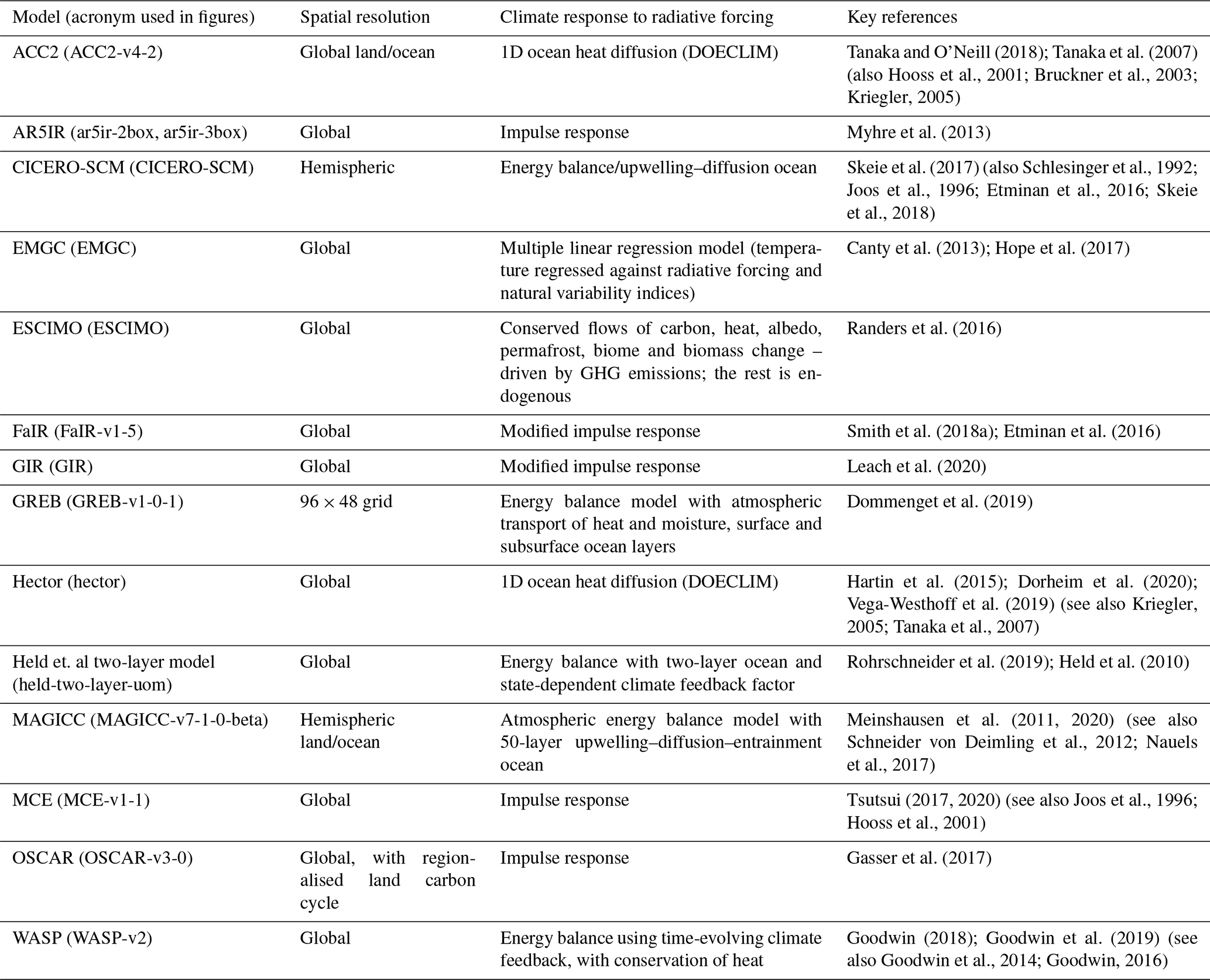
An ongoing comprehensive evaluation and assessment of RCMs requires an established protocol. The Reduced Complexity Model Intercomparison Project (RCMIP) proposed here provides such a protocol (also see https://www.rcmip.org/, last access: 22 October 2020). In the RCMIP community call (available at https://www.rcmip.org/, last access: 22 October 2020) RCMs were broadly defined as follows: “[…] RCMIP is aimed at reduced-complexity, simple climate models and small emulators that are not part of the intermediate complexity EMIC or complex GCM/ESM categories”. In practice, we encouraged any group in the scientific community who identifies with the label of RCM to participate in RCMIP; see Table 1 for an overview of the models which participated in RCMIP Phase 1.
Tanaka and O'Neill (2018); Tanaka et al. (2007)Hooss et al., 2001; Bruckner et al., 2003; Kriegler, 2005Myhre et al. (2013)Skeie et al. (2017)Schlesinger et al., 1992; Joos et al., 1996; Etminan et al., 2016; Skeie et al., 2018Canty et al. (2013); Hope et al. (2017)Randers et al. (2016)Smith et al. (2018a); Etminan et al. (2016)Leach et al. (2020)Dommenget et al. (2019)Hartin et al. (2015); Dorheim et al. (2020); Vega-Westhoff et al. (2019)Kriegler, 2005; Tanaka et al., 2007Rohrschneider et al. (2019); Held et al. (2010)Meinshausen et al. (2011, 2020)Schneider von Deimling et al., 2012; Nauels et al., 2017Tsutsui (2017, 2020)Joos et al., 1996; Hooss et al., 2001Gasser et al. (2017)Goodwin (2018); Goodwin et al. (2019)Goodwin et al., 2014; Goodwin, 2016Table 1Models participating in RCMIP Phase 1. Note that GIR has since been renamed FaIR-v2-0-0.
We aim for RCMIP to provide a focal point for further development and an experimental design which allows models to be readily compared and contrasted, mirroring the regular comparisons which are performed for AOGCMs and ESMs in each of CMIP's iterations. We intend for RCMIP to facilitate more regular and targeted assessment of RCMs.
Thus, whilst RCMIP mirrors many of the experimental setups developed within CMIP6, RCMIP focuses on RCMs and is hence not one of the official CMIP6 (Eyring et al., 2016) endorsed intercomparison projects (that are instead targeted at ESMs). Nonetheless, RCMs are part of the climate model hierarchy, so we aim to make comparing the RCMIP results with results from other modelling communities, specifically CMIP, as simple as possible. Accordingly, RCMIP replicates selected experimental designs of many of the CMIP-endorsed MIPs, particularly the DECK (Eyring et al., 2016) and ScenarioMIP (O'Neill et al., 2016) simulations.
In what follows, we describe RCMIP Phase 1. In Sect. 2, we detail the domain of RCMIP Phase 1 and its research questions. In Sect. 3, we provide an overview of the participating models and their configuration. In Sect. 4, we describe the experimental setup. In Sect. 5 we present results from RCMIP Phase 1, before presenting possible extensions in Sect. 6 and conclusions in Sect. 7.
The key point of this paper is to introduce RCMIP, its goals and its setup. As a proof of concept, we also include key initial research questions, the implemented experimental setup and associated results from RCMIP's first phase.
2.1 Research question 1: is the reduced-complexity modelling community ready to run an intercomparison and how long would such an intercomparison take to run?
Model intercomparisons require significant effort on the part of the organising community and each of the modelling teams involved. The reduced-complexity modelling community has not undertaken such an effort previously; hence the first question is whether the community is ready to perform an intercomparison.
In addition to whether an intercomparison is possible, the second part of the first question is how long and how much effort is required to perform the intercomparison. The most successful intercomparisons are built on standardised protocols for experiment design, model setup and data handling. To date, no such standards exist for the reduced-complexity modelling community.
Here we investigate how easily the benefits of systematic intercomparison can be brought to the reduced-complexity modelling community by performing the first of many envisaged rounds of intercomparison. In the process, we gain vital insights into the effort, timelines and scope which can reasonably be managed by the participating modelling teams. Such knowledge is vital for planning future efforts.
2.2 Research question 2: can reduced-complexity climate models capture observed historical global-mean surface air temperature (GSAT) trends?
The second research question focuses on a key metric for evaluating RCMs against observations. This research question evaluates the extent to which each RCM's approximations and parameterisations cause its response to deviate from observational data.
However, given the limited amount of observations available, comparing only with observations leaves us with little understanding of how RCMs perform in scenarios apart from a historical one in which anthropogenic emissions are heating the climate. Recognising that there are a range of possible futures, it is vital to also assess RCMs in other scenarios. Prominent examples include stabilising or falling anthropogenic emissions, strong mitigation of non-CO2 climate forcers and scenarios with CO2 removal. The limited observational set motivates RCMIP's third research question: evaluation against more complex models.
2.3 Research question 3: to what extent can reduced-complexity models emulate the global-mean temperature response of more complex models?
Whilst the response of more comprehensive models may not represent the behaviour of the actual Earth system, they are the best available representation of our understanding of the Earth system's physical processes. By evaluating RCMs against more complex models, we can quantify the extent to which the simplifications made in RCMs limit their ability to capture physically based model responses – for example the extent to which the approximation of a constant climate feedback in some RCMs limits the RCM's ability to replicate ESMs' longer-term response under either higher forcing or lower overshoot scenarios (Rohrschneider et al., 2019).
2.4 Research question 4: what can a multi-model ensemble of RCMs tell us about the difference between the SSP-based and RCP scenarios?
The SSP-based scenarios (O'Neill et al., 2016; Riahi et al., 2017) are the cornerstone of CMIP6's ScenarioMIP and are an update of CMIP5's RCP scenarios (van Vuuren et al., 2011a). One of the key intents behind some of the SSP-based scenarios is that they share the same nameplate 2100 radiative forcing level as the RCPs (e.g. ssp126 and rcp26, ssp245 and rcp45), the idea being that they would have similar climatic outcomes despite their different atmospheric concentration inputs. However, the nameplate radiative forcing comparisons between RCPs and SSPs were undertaken on the basis of IPCC AR5-consistent stratospheric-adjusted radiative forcings (Myhre et al., 2013). Taking into account new insights into respective CO2 and CH4 forcings, as well as effective radiative forcings, different climate responses can be expected. In fact, Wyser et al. (2020) suggest that the difference in atmospheric concentrations results in non-trivial differences in climate projections.
Unfortunately, evaluating the scenario differences between RCP and SSP-based scenarios with a large, identical set of CMIP models is difficult because of the computational cost (many CMIP6 modelling groups will not perform all CMIP6 ScenarioMIP experiments, let alone performing extra CMIP5 experiments). With an ensemble of RCMs, we can provide further insight into how much the change in emissions pathways affects climate projections using identical models, building on the insights from the CMIP groups which can afford to run the required experiments. In addition, RCMs also offer one other benefit: they can diagnose effective radiative forcing directly. As a result, RCMs can provide more detailed insights into the reasons for differences because they provide a more detailed breakdown of the emissions–climate change cause–effect chain. In contrast, diagnosing effective radiative forcing from CMIP models is a difficult task which requires a number of extra experiments, all of which come at additional computational cost (Smith et al., 2020).
2.5 Research question 5: how does the relationship between cumulative CO2 emissions and global-mean temperature vary both between RCMs and within a parameter ensemble of an RCM?
The relationship between cumulative CO2 emissions and global-mean temperature is key to deriving the transient climate response to emissions (IPCC, 2018), a key metric in the calculation of our remaining carbon budget (Rogelj et al., 2019). Here we investigate how this relationship varies between RCMs and within a parameter ensemble from a given RCM. Whilst a multi-model ensemble demonstrates variance due to model structure, the parameter ensemble demonstrates variance that arises solely as a result of changes in the strength of the response of individual components. These insights build on results from experiments with more complex models (see e.g. Arora et al., 2020), which cannot perform such large perturbed parameter ensembles because of computational cost.
Fifteen models have participated in RCMIP Phase 1 (see Table 1 for an overview and links to key description papers; note that GIR has been renamed FaIR-v2 since the preparation of this paper). We encourage any other interested groups to join further phases of the project.
Even within the reduced-complexity category, there is considerable variation in both model complexity and the number of climate components (Table 1). At the simplest end, we have the radiative-forcing-driven (see Sect. 4) impulse response models, represented by the AR5IR model variants. These models project global-mean temperature only and, in the setup submitted here, provide only annual-mean values (although they can be run at higher temporal resolution if desired). At the other end of the spectrum, we have MAGICC, which includes representations of 43 greenhouse gas cycles, includes parameterisations of the relationship between aerosol emissions and aerosol effective radiative forcing, distinguishes between different hemispheres and land/ocean regions of the globe, has 50 ocean layers in each hemisphere, and runs on a monthly time step internally (although all output is annual mean only). Some models take a more hybrid approach, increasing complexity in only a single component whilst retaining simplicity elsewhere. Examples of increased complexity in specific domains include OSCAR's regionalised land carbon cycle and EMGC's representation of natural variability.
An in-depth description of these models and their differences is beyond the scope of this paper (but is planned for future research). For readers interested in the details of all the participating models, we refer to the references provided in Table 1.
3.1 Model configuration
RCMs are usually highly flexible. Their response to anthropogenic and natural drivers strongly depends on the configuration in which they are run (i.e. their parameter values). In RCMIP Phase 1, we have requested that all models provide one set of simulations in which their equilibrium climate sensitivity is equal to 3 ∘C. Whilst this does not define the entirety of a model's behaviour, it removes a major cause of difference between model output which is not related to model structure. Within Phase 1 of RCMIP, we have given modelling groups the freedom to choose whether they apply any additional constraints or not.
On top of the 3 ∘C climate sensitivity configuration, we have also invited groups to submit two other configuration categories. The first is any other best guess or default configurations, where each participating modelling group is free to choose their own best guess (the details of which can be found in the references provided in Table 1). The second is configurations deliberately designed to emulate specific ESMs from CMIP5 and CMIP6. Given the complexities involved in calibration (see e.g. Meinshausen et al., 2011; Tsutsui, 2020), not all modelling groups submitted such CMIP5- and CMIP6-specific configurations. However, for those groups that did, these emulation setups provide valuable insight into the extent to which the model's structure limits its ability to reproduce the behaviour of more complex models. Given the complexity of the topic, we leave decisions about how to calibrate their model up to the individual modelling teams (details of each group's approach can be found in the references provided in Table 1). A more top-down approach will be undertaken in a future phase of RCMIP (see Sect. 6).
RCMs generally model multiple steps in the emissions–climate change cause–effect chain, including gas cycles (emissions-to-concentration step), radiative forcing parameterisations (concentrations-to-radiative-forcing step) and temperature response (radiative-forcing-to-warming step). Here, effective radiative forcing and radiative forcing are defined following Myhre et al. (2013). In contrast to radiative forcing, effective radiative forcing includes rapid adjustments beyond stratospheric temperature adjustments and thus is a better indicator of long-term climate change.
Each point in the chain can be used as the starting point for simulations; i.e. the simulation might be defined in terms of prescribed concentrations, emissions or radiative forcing. In Phase 1 of RCMIP, we focus on experiments which are defined in terms of concentrations to facilitate a direct comparison with CMIP experiments, most of which are also defined in terms of concentrations.
RCMIP Phase 1 focuses on 19 experiments, which can be broken down into two categories: scenario-based and idealised. We provided all inputs following, and requested that all outputs follow, a standard format to facilitate ease of data analysis and re-use (Sect. S1 in the Supplement). This common data format was developed for RCMIP and combines elements of the integrated assessment community standard (Gidden and Huppmann, 2019) and the CMIP6 definitions of variables and scenarios.
4.1 Scenario-based experiments
Scenario-based experiments examine model responses to historical transient forcing as well as a range of future scenarios. The historical experiments provide a way to compare RCM output against observational data records (research question 2) and are complementary to the idealised experiments (Sect. 4.2), which provide a cleaner assessment of model response to forcing. The future scenarios probe RCM responses to a range of possible climate futures, both continued warming and stabilisation or overshoots in forcing. The variety of scenarios is a key test of model behaviour, evaluating them over a range of conditions rather than only over the historical period. Direct comparison with CMIP output then provides information about the extent to which the simplifications involved in RCM modelling are able to reproduce the response of the most advanced physically based ESMs (research question 3).
RCMIP Phase 1's scenario experiments are historical, ssp119, ssp126, ssp245, ssp370, ssp434, ssp460, ssp534-over, ssp585, rcp26, rcp45, rcp60 and rcp85. We focus on simulations (historical plus future) which cover the range in forcing scenarios from the CMIP6 ScenarioMIP exercise (O'Neill et al., 2016; Riahi et al., 2017) and CMIP5 RCP scenarios (van Vuuren et al., 2011a). These quickly reveal differences in model projections over the widest available scenario range which can also be compared to CMIP6 output. The CMIP5 experiments are particularly useful as they provide a direct comparison between CMIP5 and CMIP6 scenarios (research question 4), something which has only been done to a limited extent with more complex models (Wyser et al., 2020).
All of these experiments are defined in terms of concentrations of well-mixed greenhouse gases. Here, “well-mixed greenhouse gases” refer to CO2, CH4, N2O, hydrofluorocarbons (HFCs), perfluorocarbons (PFCs) and hydrochlorofluorocarbons (HCFCs). However, scenario experiments include more than just well-mixed greenhouse gases, so these concentrations are supplemented by aerosol precursor species emissions, ozone-relevant emissions and natural effective radiative forcing variations. Here, “aerosol precursor species emissions” refer to emissions of sulfur, nitrates, black carbon, organic carbon and ammonia. “Ozone-relevant emissions” refer to emissions of carbon monoxide and non-methane volatile organic compounds (NMVOCs). For models which do not include the steps of aerosol emissions to effective radiative forcing or ozone-relevant emissions to ozone effective radiative forcing, prescribed effective radiative forcings can instead be used. Here “natural effective radiative forcing variations” refer to effective radiative forcing due to natural volcanic eruptions and changes in solar irradiance. All data sources are described in Sect. S2.
The key difference between the RCMIP experiments and the CMIP experiments is that some RCMs include more anthropogenic drivers than CMIP models. Specifically, CMIP models do not include the full range of HFC, PFC and HCFC species, instead using equivalent concentrations (Meinshausen et al., 2017, 2020). In addition, some CMIP models will not include the effect of aerosol precursors such as nitrates, ammonia and organic carbon (McCoy et al., 2017).
4.2 Idealised experiments
In addition to the scenario-based experiments, RCMIP Phase 1 also includes a number of idealised experiments. All of these experiments are defined in terms of CO2 concentrations alone. These experiments provide an easy point of comparison with output from other models, particularly CMIP output, as well as information about basic model behaviour and dynamics which can be useful for understanding the differences between models.
RCMIP Phase 1's idealised experiments are 1pctCO2, 1pctCO2-4xext, abrupt-4xCO2, abrupt-2xCO2 and abrupt-0p5xCO2. These examine the RCMs' response to a 1 % yr−1 increase in atmospheric CO2 concentrations (1pctCO2); 1pctCO2 followed by constant CO2 concentrations once atmospheric CO2 concentrations quadruple (1pctCO2-4xext); and abrupt changes in atmospheric CO2 to 4 times pre-industrial levels (abrupt-4xCO2), double pre-industrial levels (abrupt-2xCO2) and half pre-industrial levels (abrupt-0p5xCO2) – mirroring the respective CMIP experiments (Eyring et al., 2016).
The experiments reveal differences in model response to forcing, particularly whether the RCM response to forcing includes non-linearities. In addition, these experiments also provide a direct comparison with CMIP experiments (i.e. more complex model behaviour) and are a key benchmark when examining an RCM's ability to emulate more complex models (research question 3). In these concentration-driven experiments, RCMs report emissions (often referred to as “inverse emissions”) and carbon cycle behaviour consistent with the prescribed CO2 pathway. These inverse emissions are key to exploring the variation in the relationship between surface air temperature change and cumulative emissions of CO2 (Allen et al., 2009; Matthews et al., 2009; Meinshausen et al., 2009; Zickfeld et al., 2009) over a range of models and parameter values (research question 5).
4.3 Output variables
Phase 1 of RCMIP focuses on five key output variables. The focus on a limited set allows us to discern major differences between RCMs and provides insights into the reasons for such differences. The first variable of interest is surface air temperature change. We choose this variable because it is comparable to available observations and CMIP output and is also policy-relevant.
In addition to surface air temperature change, we request total, anthropogenic, CO2 and aerosol effective radiative forcing. These forcing variables are key indicators of the long-term drivers of climate change within each model as well as being key metrics for the IAM community. In particular, aerosol effective radiative forcing is highly uncertain and a key source of difference between RCMs.
The final variable we request is CO2 emissions. Given that all our experiments are defined in terms of concentrations, we request CO2 emissions compatible with the prescribed CO2 pathways.
Within 3 months of beginning RCMIP and publishing the protocols, 15 different RCMs submitted data. Given that this is the first phase of RCMIP, we expect even shorter turnarounds in future. The submitted results demonstrate that the RCM community, via RCMIP, now has the capacity to run multi-model studies, and to run them comparatively quickly. In addition, the number of participating modelling groups demonstrates that the RCMIP infrastructure is accessible to a wide range of modelling teams.
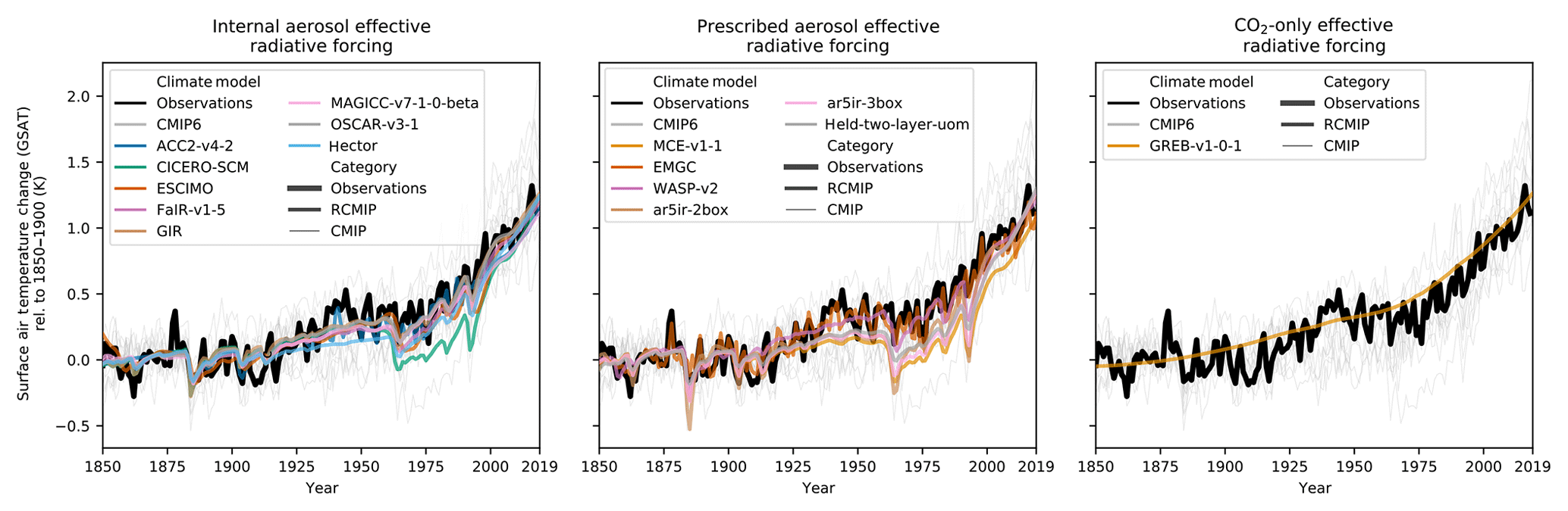
Figure 1Historical global-mean annual mean surface air temperature (GSAT) simulations. Thick black line is observed GSAT (Richardson et al., 2016; Rogelj et al., 2019). Medium-thickness lines are default configurations for RCMIP models. Thin grey solid lines are CMIP6 models. In order to provide time series up until 2019, we have used data from the combination of historical and ssp585 simulations.
All the RCMs are able to capture the approximately 1 ∘C of warming seen in the historical observations (Fig. 1), compared to a pre-industrial reference period (Richardson et al., 2016; Rogelj et al., 2019). However, the RCMs vary in the detail which they represent. Most of the RCMs include some representation of the impact of volcanic eruptions, most notably the drop in global-mean temperatures after the eruption of Mount Agung in 1963. In addition, most of the RCMs do not capture natural variability driven by processes such as the El Niño–Southern Oscillation (Wolter and Timlin, 2011), the Pacific Decadal Oscillation (Zhang et al., 1997) and the Indian Ocean Dipole (Saji et al., 1999). The exception to this is the EMGC model, which includes representations of the impact of all of these processes. At the other end of the complexity spectrum, we have the CO2-only model, GREB. Unlike the other RCMs, GREB lacks the volcanic and aerosol-induced cooling signals of the 19th and 20th centuries.
Table 2Model emulation scores over all emulated models and scenarios. Here we provide root-mean-square errors over the SSPs plus four idealised CO2-only experiments (abrupt-2xCO2, abrupt-4xCO2, abrupt-0p5xCO2, 1pctCO2). As the models have not all provided emulations for the same set of target models and scenarios, the model emulation scores are indicative only and are not a true, fair test of skill. For target model by target model emulation scores, see Table S1.
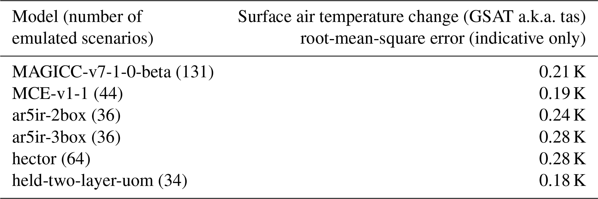

Figure 2Emulation of CMIP6 models by RCMs. The thick transparent lines are the target CMIP6 model output (here from IPSL-CM6A-LR r1i1p1f1). The thin lines are emulations from different RCMs. Panel (a) shows results for scenario-based experiments, whilst panels (b)–(e) show results for idealised CO2-only experiments (note that panels b–e share the same legend). See the Supplement for other target CMIP6 models.
RCMIP also facilitates a comparison of model calibrations and CMIP output (Fig. 2). Examining multiple emulation setups, we see that RCMs can reproduce the temperature response of CMIP models to forcing changes to within a root-mean-square error of 0.2 ∘C (Table 2). A detailed comparison of RCMs with 24 CMIP6 ESM ensemble members is available in the Supplement (Table S1 and Figs. S1–S24). In scenario-based experiments, it appears to be harder for RCMs to emulate CMIP output than in idealised experiments. We suggest two key explanations. The first is that effective radiative forcing cannot be easily diagnosed in SSP-based scenarios and hence it is hard to know how best to force the RCM during calibration. The second is that the forcing in these scenarios includes periods of increase, sudden decrease due to volcanoes and longer-term stabilisation rather than the simpler changes seen in the idealised experiments. Fitting all three of these regimes is a more difficult challenge than fitting the idealised experiments alone.
Only 6 models (Table 2) have been able to submit emulation configurations. Furthermore, each RCM is calibrated to a different number of CMIP models, with some modelling teams unable to provide any calibrations at all. The reason is that there is to date no common resource of calibration data from the CMIP6 repositories. The technical challenge of diagnosing, stitching together, creating area-weighted averages and de-drifting a large amount of CMIP6 output data within a short time period has turned out to be a hurdle for many modelling teams. As an offspring from RCMIP, we attempt to address this challenge for the future by providing a unifying data portal (see https://cmip6.science.unimelb.edu.au/, last access: 22 October 2020, Nicholls et al., 2020b).
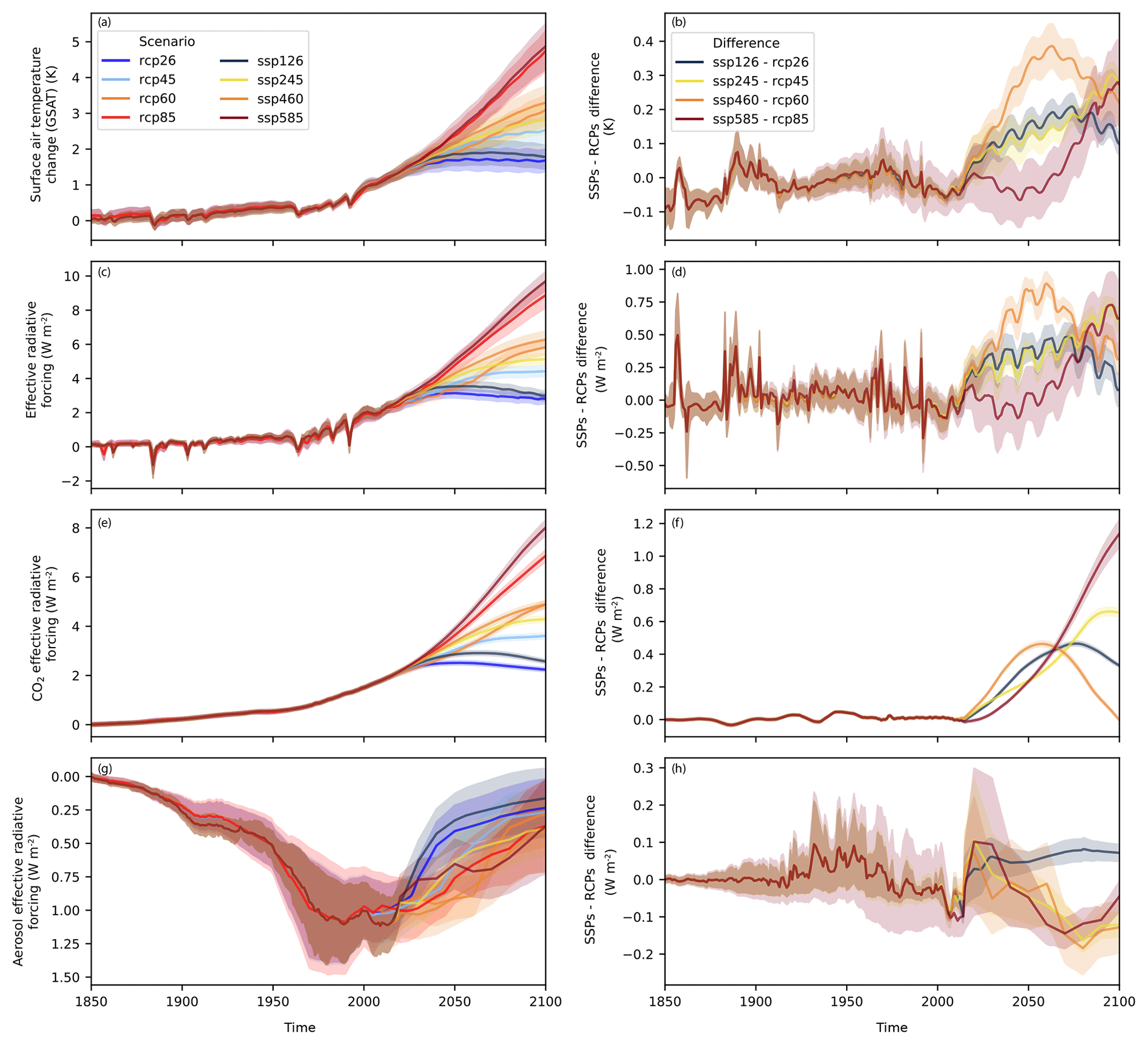
Figure 3Output from the RCP and SSP-based scenarios up until 2100. The left-hand column shows raw model output. The right-hand column shows the difference between RCP and SSP-based scenario pairs for a given model's output. The shaded range shows 1 standard deviation about the median (solid lines). Output is shown for surface air temperature change (GSAT, a and b), effective radiative forcing (c and d), CO2 effective radiative forcing (e and f) and aerosol effective radiative forcing (g and h). The results here are based on a limited set of models: CICERO-SCM, MAGICC, OSCAR, GIR (since renamed FaIR-v2) and FaIR. Only these models have performed the required RCP and SSP-based scenario pair experiments.
The ensemble of RCMs also provides insights into the differences between CMIP5 and CMIP6 generation scenarios (“RCP” and “SSP-based” scenarios respectively) when these scenarios are run with identical models (Fig. 3). In the selection of models which have submitted all RCP and SSP-based scenario pairs, the SSP-based scenarios are 0.20 ∘C (standard deviation 0.10 ∘C across the available models) warmer than their corresponding RCPs (Fig. 3b). This difference is driven by the 0.39 ±0.24 W m−2 larger effective radiative forcing in the SSP-based scenarios (Fig. 3d), which itself is driven by the 0.53±0.44 W m−2 larger CO2 effective radiative forcing in the SSP-based scenarios (Fig. 3f). These results add to the work of Wyser et al. (2020), which suggests that, even when run with the same model (in a concentration-driven setup), the SSP-based scenarios result in warmer projections than the RCPs. When we run one of the RCMs (MAGICC) with an AR5-consistent stratospheric-adjusted radiative forcing definition (Myhre et al., 2013), the SSP-based and RCP scenarios are within 6 % of each other in 2100 (although their AR5-consistent stratospheric-adjusted radiative forcing trajectories can differ by up to 15 % at different times over the 21st century). Thus, we find that the update to effective radiative forcing (Forster et al., 2016), mainly using the formulations presented in Etminan et al. (2016) plus any rapid adjustment terms (Smith et al., 2018b), increases the total forcing in the SSP-based scenarios, because their generally higher CO2 concentrations are partially, but not fully, offset by lower CH4 concentrations (see e.g. Fig. 11 in Meinshausen et al., 2020). There is a clear need for further, more comprehensive exploration of the differences between the RCP and SSP-based scenarios.
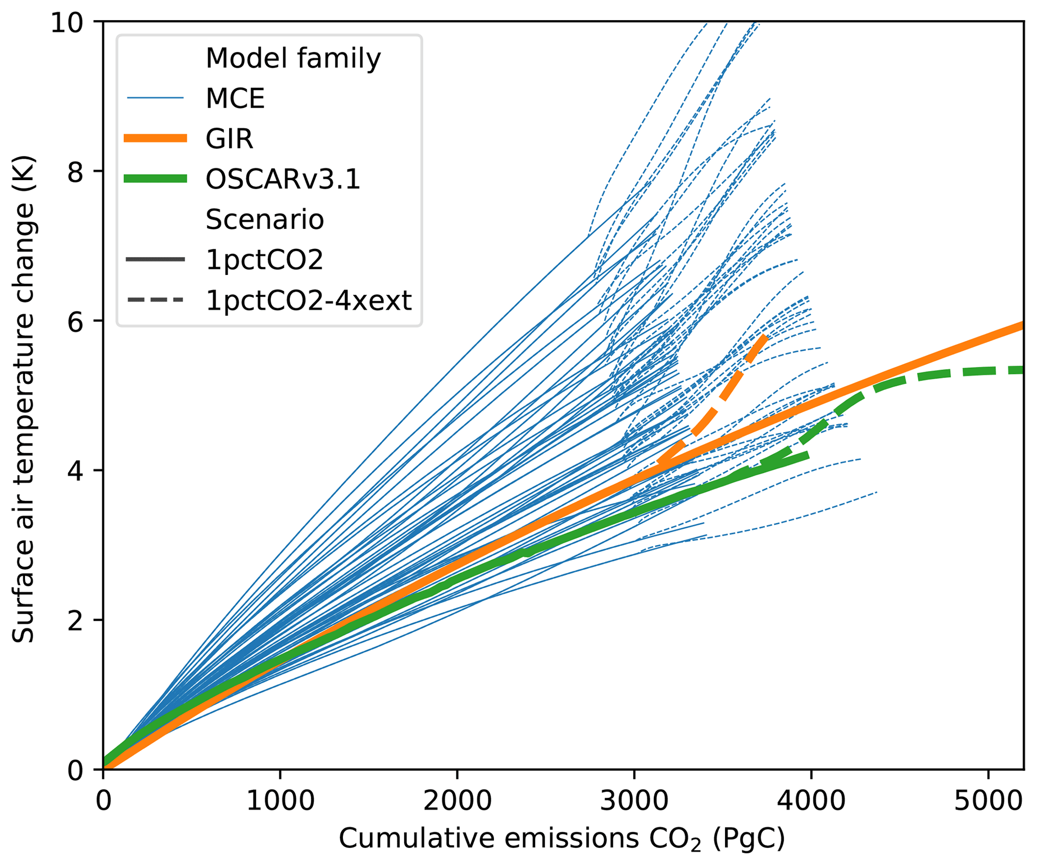
Figure 4Surface air temperature change against cumulative CO2 emissions in the 1pctCO2 and 1pctCO2-4xext experiments. Thin lines are used for the MCE model's family of emulation setups. Thick lines are used for the GIR (since renamed FaIR-v2) and OSCAR 3 ∘C climate sensitivity setups.
Finally, we present variations in the relationship between surface air temperature change and cumulative CO2 emissions from the 1pctCO2 and 1pctCO2-4xext experiments (Fig. 4). To date, only three models (GIR (since renamed FaIR-v2), MCE and OSCAR) have been able to provide the required outputs (in particular deriving inverse emissions from these concentration-defined experiments). From the available results, it is clear that the relationship between these two key variables varies over MCE's parameter ensemble, from weakly sub-linear to weakly super-linear. Such variation can have notable implications for the remaining carbon budget (Nicholls et al., 2020a). We also see that the MCE model's parameter ensemble covers a large range, dwarfing the differences between it and the GIR (since renamed FaIR-v2) and OSCAR models, which are shown here in their 3 ∘C climate sensitivity configurations. This suggests that, at least for RCMs, the response of individual components and their configuration is more important than model structure, although this conclusion is tempered by the paucity of available results.
RCMIP Phase 1 provides proof of concept of the RCMIP approach to RCM evaluation, comparison and examination. However, Phase 1 has been limited to a very specific set of questions, and there is wide scope to use RCMs to examine other scientific questions of interest. In this section we present a number of ways in which further research and phases of RCMIP could build on the work presented in this paper.
The first is an exploration of probabilistic outputs. Most RCMs can be calibrated, i.e. have their parameters adjusted, such that they reproduce our best-estimate (typically median) observations. However, RCMs are also used in a probabilistic mode. In this mode a parametric ensemble is run for a given RCM and set of climate forcers. The results are then used to capture the likelihood that different climate changes will unfold, particularly the likelihood of reaching different warming levels. Given the widespread use of probabilistic distributions, particularly for quantifying likely ranges of climate sensitivity and climate projections (see e.g. Meinshausen et al., 2009; Skeie et al., 2018; Vega-Westhoff et al., 2019), examining the differences between existing probabilistic model setups is an obvious next step.
Secondly, there are a wide range of RCMs available in the literature. This variety can be confusing, especially to those who are not intimately involved in developing the models. An overview of the different models, their structure and relationship to one another (in the form of a genealogy) would help reduce the confusion and provide clarity about the implications of using one model over another.
Thirdly, emulation results have generally only been submitted for a limited set of experiments. Hence it is still not clear whether the emulation performance seen in idealised experiments also carries over to scenarios, particularly the SSP-based scenarios. As the number of available CMIP6 results continues to grow, this area is ripe for investigation and will lead to improved understanding of the limits of the reduced-complexity approach. The development of a common resource (see https://cmip6.science.unimelb.edu.au/, last access: 22 October 2020; Nicholls et al., 2020b) for RCM calibration will greatly aid this effort by ensuring that each group has access to the same set of calibration data.
Finally, whilst evaluating RCMs is a useful exercise, the root causes of these differences may not be clear. This can be addressed by performing experiments which specifically diagnose the reasons for differences between models, for example simple pulse emissions of different species or prescribed step changes in atmospheric greenhouse gas concentrations. Such experiments could build on existing research (van Vuuren et al., 2011b; Schwarber et al., 2019) and would allow even more comprehensive examination and understanding of RCM behaviour. This would require custom experiments, particularly for the carbon cycle, which is strongly coupled to other parts of the climate system. However, unlike in the case of ESMs, adding extra RCM experiments adds relatively little technical or human burden, because RCMs are computationally cheap and because RCMIP's standardised formats facilitate highly automated experiment pipelines.
RCMs are used in many applications, particularly where computational constraints prevent other techniques from being used. Due to their importance in climate policy assessments and in carbon budget calculations, as well as their applicability to a wide range of scientific questions, understanding the behaviour and output from RCMs is highly relevant and requires continuous updating with the latest science. Here we have presented the Reduced Complexity Model Intercomparison Project (RCMIP), an effort to facilitate the evaluation and understanding of RCMs in a systematic, standardised and detailed way. We hope this can greatly improve ease of use of, and familiarity with, RCMs.
We have performed RCMIP Phase 1, which provides an initial database of experiments conducted with 15 participating models from the RCM community. RCMIP Phase 1 focused on basic comparisons of RCMs with observed global-mean temperature changes, comparisons of RCMs with the global-mean temperature response of more complex models, the difference between the SSP-based and RCP scenarios, and an exploration of the relationship between cumulative CO2 emissions and surface air temperature change in the RCMs. These initial comparisons demonstrate that RCMIP's infrastructure is a useful tool for such intercomparisons and that the RCM community is able to perform such intercomparisons on timescales of the order of months. Further work will examine the relationship between different RCMs, RCMs' probabilistic projections and the cause of differences between RCMs.
RCMIP fills a gap in our understanding of RCM behaviour, in particular, how different RCMs perform relative to each other as well as how they compare with observations. This gap is particularly important to fill given the widespread use of RCMs throughout the integrated assessment modelling community and in large-scale climate science assessments. We welcome requests, suggestions and further involvement from throughout the climate modelling research community. With our efforts, we aim to increase understanding of and confidence in RCMs, particularly for their many users at the science–policy interface.
RCMIP input time series and results data along with processing scripts as used in this submission are available from the RCMIP GitLab repository at https://gitlab.com/rcmip/rcmip (last access: 22 October 2020) and archived by Zenodo (https://doi.org/10.5281/zenodo.3593569, Nicholls and Gieseke, 2019).
The ACC2 model code is available upon request.
The implementation of the AR5IR model used in this study is available in the OpenSCM repository: https://github.com/openscm/openscm/blob/ar5ir-notebooks/notebooks/ar5ir_rcmip.ipynb (last access: 22 October 2020, Nicholls, 2020).
The model version of ESCIMO used to produce the RCMIP runs can be downloaded from http://www.2052.info/wp-content/uploads/2019/12/mo191107%202%20ESCIMO-rcimp from%20mo160911%202100%20ESCIMO.vpm (last access: 22 October 2020, Randers et al., 2020). The vpm extension allows you to view, examine and run the model but not save it. The original model with full documentation is available from http://www.2052.info/escimo/ (last access: 22 October 2020).
FaIR is developed on GitHub at https://github.com/OMS-NetZero/FAIR (last access: 22 October 2020), and v1.5 used in this study is archived at Zenodo (Smith et al., 2019).
The GREB model source code used is available, upon request, on Bitbucket: https://bitbucket.org/rcmipgreb/greb-official/src/official-rcmip/ (last access: 22 October 2020). The last stable versions are available on GitHub at https://github.com/christianstassen/greb-official/releases (last access: 22 October 2020, Stassen et al., 2020).
The Held et al. two-layer model implementation used in this study is available in the OpenSCM repository: https://github.com/openscm/openscm/blob/ar5ir-notebooks/notebooks/held_two_layer_rcmip.ipynb.
Hector is developed on GitHub at https://github.com/JGCRI/hector (last access: 22 October 2020). The exact version of Hector used for these simulations can be found at https://github.com/ashiklom/hector/releases/tag/rcmip-phase-1 (last access: 22 October 2020, Link et al., 2020). The scripts for the RCMIP runs are available at https://github.com/ashiklom/hector-rcmip (last access: 22 October 2020, Link et al., 2020).
MAGICC's Python wrapper is archived at Zenodo (https://doi.org/10.5281/zenodo.1111815, Nicholls et al., 2019) and developed on GitHub at https://github.com/openclimatedata/pymagicc/ (last access: 22 October 2020).
OSCAR v3 is available on GitHub at https://github.com/tgasser/OSCAR (lasty access: 22 October 2020, Gasser, 2020).
WASP's code for the version used in this study is available from the supplement of Goodwin (2018): https://doi.org/10.1029/2018EF000889. See also the WASP website at https://waspclimatemodel.info/downloads/ (last access: 22 October 2020).
The other participating models are not yet available publicly for download or as open source. Please also refer to their respective model description papers for notes and code availability.
The supplement related to this article is available online at: https://doi.org/10.5194/gmd-13-5175-2020-supplement.
ZN and RG conceived the idea for RCMIP. ZN, MM and JL set up the RCMIP website (https://www.rcmip.org/, last access: 22 October 2020), produced the first draft of the protocol and derived the data format. All authors contributed to updating and improving the protocol. ACC2 results were provided by KT and EK. AR5IR and Held et al. two-layer model were provided by ZN. CICERO-SCM results were provided by JF, BS, MS and RBS. EMGC results were provided by LM, AH and RJS. ESCIMO results were provided by UG. FaIR results were provided by CS. GIR results were provided by NL. GREB results were provided by DD, CF, DM and ZX. Hector results were provided by AS and KD. MAGICC results were provided by MM, JL and ZN. MCE results were provided by JT. OSCAR results were provided by TG and YQ. WASP results were provided by PG. ZN wrote, except for the model descriptions, the first manuscript draft, produced all the figures and led the manuscript writing process with support from RG. All authors contributed to writing and revising the manuscript.
The authors declare that they have no conflict of interest.
We acknowledge the World Climate Research Programme, which, through its Working Group on Coupled Modelling, coordinated and promoted CMIP6. We thank the climate modelling groups for producing and making available their model output, the Earth System Grid Federation (ESGF) for archiving the data and providing access, and the multiple funding agencies who support CMIP6 and ESGF. RCMIP could not go ahead without the outputs of CMIP6 nor without the huge effort which is put in by all the researchers involved in CMIP6 (some of whom are also involved in RCMIP).
We also thank the RCMIP Steering Committee – comprised of Maisa Corradi, Piers Forster, Jan Fuglestvedt, Malte Meinshausen, Joeri Rogelj and Steven Smith – for their support and guidance throughout Phase 1. We look forward to their ongoing support in further phases.
Katsumasa Tanaka is supported by the Integrated Research Program for Advancing Climate Models (TOUGOU Program), the Ministry of Education, Culture, Sports, Science, and Technology (MEXT), Japan.
Zebedee R. J. Nicholls has been supported by the ARC Centre of Excellence for Climate Extremes (grant no. CE170100023). Katsumasa Tanaka benefited from state assistance managed by the National Research Agency in France under the “Programme d’Investissements d’Avenir” under the reference “ANR-19-MPGA-0008”. Robert Gieseke has been supported by the German Federal Ministry for the Environment, Nature Conservation and Nuclear Safety (grant no. NO16_II_148_Global_A_IMPACT) while at PIK in the beginning of RCMIP. The EMGC work was supported by the NASA Climate Indicators and Data Products for Future National Climate Assessments (INCA) programme (award NNX16AG34G).
This paper was edited by Carlos Sierra and reviewed by three anonymous referees.
Allen, M. R., Frame, D. J., Huntingford, C., Jones, C. D., Lowe, J. A., Meinshausen, M., and Meinshausen, N.: Warming caused by cumulative carbon emissions towards the trillionth tonne, Nature, 458, 1163–1166, 2009. a
Arora, V. K., Katavouta, A., Williams, R. G., Jones, C. D., Brovkin, V., Friedlingstein, P., Schwinger, J., Bopp, L., Boucher, O., Cadule, P., Chamberlain, M. A., Christian, J. R., Delire, C., Fisher, R. A., Hajima, T., Ilyina, T., Joetzjer, E., Kawamiya, M., Koven, C. D., Krasting, J. P., Law, R. M., Lawrence, D. M., Lenton, A., Lindsay, K., Pongratz, J., Raddatz, T., Séférian, R., Tachiiri, K., Tjiputra, J. F., Wiltshire, A., Wu, T., and Ziehn, T.: Carbon–concentration and carbon–climate feedbacks in CMIP6 models and their comparison to CMIP5 models, Biogeosciences, 17, 4173–4222, https://doi.org/10.5194/bg-17-4173-2020, 2020. a
Bruckner, T., Hooss, G., Füssel, H.-M., and Hasselmann, K.: Climate System Modeling in the Framework of the Tolerable Windows Approach: The ICLIPS Climate Model, Clim. Change, 56, 119–137, https://doi.org/10.1023/a:1021300924356, 2003. a
Canty, T., Mascioli, N. R., Smarte, M. D., and Salawitch, R. J.: An empirical model of global climate – Part 1: A critical evaluation of volcanic cooling, Atmos. Chem. Phys., 13, 3997–4031, https://doi.org/10.5194/acp-13-3997-2013, 2013. a
Carlson, D. and Eyring, V.: Contributions to Climate Science of the Coupled Model Intercomparison Project, available at: https://public.wmo.int/en/resources/bulletin/contributions-climate-science-of-coupled-model-intercomparison-project (last access: 22 October 2020), 2017. a
Clarke, L., Jiang, K., Akimoto, K., Babiker, M., Blanford, G., Fisher-Vanden, K., Hourcade, J.-C., Krey, V., Kriegler, E., Löschel, A., McCollum, D., Paltsev, S., Rose, S., Shukla, P. R., Tavoni, M., van der Zwaan, B., and van Vuuren, D. P: Assessing Transformation Pathways, in: Climate Change 2014: Mitigation of Climate Change, Contribution of Working Group III to the Fifth Assessment Report of the Intergovernmental Panel on Climate Change, edited by: Edenhofer, O., Pichs-Madruga, R., Sokona, Y., Farahani, E., Kadner, S., Seyboth, K., Adler, A., Baum, I., Brunner, S., Eickemeier, P., Kriemann, B., Savolainen, J., Schlömer, S., von Stechow, C., Zwickel, T., and Minx, J. C., Cambridge University Press, 413–510, 2014. a
Dommenget, D., Nice, K., Bayr, T., Kasang, D., Stassen, C., and Rezny, M.: The Monash Simple Climate Model experiments (MSCM-DB v1.0): an interactive database of mean climate, climate change, and scenario simulations, Geosci. Model Dev., 12, 2155–2179, https://doi.org/10.5194/gmd-12-2155-2019, 2019. a
Dorheim, K., Link, R., Hartin, C., Kravitz, B., and Snyder, A.: Calibrating simple climate models to individual Earth system models: Lessons learned from calibrating Hector, Earth Space Sci., https://doi.org/10.1029/2019ea000980, 2020. a
Etminan, M., Myhre, G., Highwood, E. J., and Shine, K. P.: Radiative forcing of carbon dioxide, methane, and nitrous oxide: A significant revision of the methane radiative forcing, Geophys. Res. Lett., 43, 12614–12623, https://doi.org/10.1002/2016gl071930, 2016. a, b, c
Eyring, V., Bony, S., Meehl, G. A., Senior, C. A., Stevens, B., Stouffer, R. J., and Taylor, K. E.: Overview of the Coupled Model Intercomparison Project Phase 6 (CMIP6) experimental design and organization, Geosci. Model Dev., 9, 1937–1958, https://doi.org/10.5194/gmd-9-1937-2016, 2016. a, b, c
Forster, P. M., Richardson, T., Maycock, A. C., Smith, C. J., Samset, B. H., Myhre, G., Andrews, T., Pincus, R., and Schulz, M.: Recommendations for diagnosing effective radiative forcing from climate models for CMIP6, J. Geophys. Res.-Atmos., 121, 12460–12475, https://doi.org/10.1002/2016JD025320, 2016. a
Forster, P., Huppmann, D., Kriegler, E., Mundaca, L., Smith, C., Rogelj, J., and Séférian, R.: Mitigation pathways compatible with 1.5 ∘C in the context of sustainable development supplementary material, IPCC/WMO, 2SM1–2SM50, available at: http://www.ipcc.ch/report/sr15/ (last access: 22 October 2020), 2018. a
Gasser, T.: OSCAR – A compact Earth system model, available at: https://github.com/tgasser/OSCAR, last access: 22 October 2020. a
Gasser, T., Ciais, P., Boucher, O., Quilcaille, Y., Tortora, M., Bopp, L., and Hauglustaine, D.: The compact Earth system model OSCAR v2.2: description and first results, Geosci. Model Dev., 10, 271–319, https://doi.org/10.5194/gmd-10-271-2017, 2017. a
Gidden, M. and Huppmann, D.: pyam: a Python Package for the Analysis and Visualization of Models of the Interaction of Climate, Human, and Environmental Systems, J. Open Sour. Softw., 4, 1095, https://doi.org/10.21105/joss.01095, 2019. a
Goodwin, P.: How historic simulation–observation discrepancy affects future warming projections in a very large model ensemble, Climate Dynam., 47, 2219–2233, https://doi.org/10.1007/s00382-015-2960-z, 2016. a
Goodwin, P.: On the Time Evolution of Climate Sensitivity and Future Warming, Earth's Future, 6, 1336–1348, https://doi.org/10.1029/2018ef000889, 2018. a, b
Goodwin, P., Williams, R. G., and Ridgwell, A.: Sensitivity of climate to cumulative carbon emissions due to compensation of ocean heat and carbon uptake, Nat. Geosci., 8, 29–34, https://doi.org/10.1038/ngeo2304, 2014. a
Goodwin, P., Williams, R. G., Roussenov, V. M., and Katavouta, A.: Climate Sensitivity From Both Physical and Carbon Cycle Feedbacks, Geophys. Res. Lett., 46, 7554–7564, https://doi.org/10.1029/2019gl082887, 2019. a
Harmsen, M. J. H. M., van Vuuren, D. P., van den Berg, M., Hof, A. F., Hope, C., Krey, V., Lamarque, J.-F., Marcucci, A., Shindell, D. T., and Schaeffer, M.: How well do integrated assessment models represent non-CO2 radiative forcing?, Clim. Change, 133, 565–582, https://doi.org/10.1007/s10584-015-1485-0, 2015. a
Hartin, C. A., Patel, P., Schwarber, A., Link, R. P., and Bond-Lamberty, B. P.: A simple object-oriented and open-source model for scientific and policy analyses of the global climate system – Hector v1.0, Geosci. Model Dev., 8, 939–955, https://doi.org/10.5194/gmd-8-939-2015, 2015. a
Held, I. M., Winton, M., Takahashi, K., Delworth, T., Zeng, F., and Vallis, G. K.: Probing the Fast and Slow Components of Global Warming by Returning Abruptly to Preindustrial Forcing, J. Climate, 23, 2418–2427, https://doi.org/10.1175/2009jcli3466.1, 2010. a
Hooss, G., Voss, R., Hasselmann, K., Maier-Reimer, E., and Joos, F.: A nonlinear impulse response model of the coupled carbon cycle-climate system (NICCS), Clim. Dynam., 18, 189–202, https://doi.org/10.1007/s003820100170, 2001. a, b
Hope, A. P., Canty, T. P., Salawitch, R. J., Tribett, W. R., and Bennett, B. F.: Forecasting Global Warming, Springer Climate, 51–114, 2017. a
Houghton, J. T., Meira Filho, L. G., Griggs, D. J., and Maskell, K.: An introduction to simple climate models used in the IPCC Second Assessment Report, Cambridge University Press Cambridge, available at: http://large.stanford.edu/courses/2015/ph240/girard1/docs/houghton.pdf (last access: 22 October 2020), 1997. a
Huppmann, D., Rogelj, J., Kriegler, E., Krey, V., and Riahi, K.: A new scenario resource for integrated 1.5 ∘C research, Nat. Clim. Change, 8, 1027–1030, https://doi.org/10.1038/s41558-018-0317-4, 2018. a
IPCC: Annex I: Glossary, in: Global Warming of 1.5 ∘C. An IPCC Special Report on the impacts of global warming of 1.5 ∘C above pre-industrial levels and related global greenhouse gas emission pathways, in the context of strengthening the global response to the threat of climate change, sustainable development, and efforts to eradicate poverty, edited by: Matthews, J. B. R., Geneva, Switzerland, in press, available at: https://www.ipcc.ch/sr15/chapter/glossary/ (last access: 22 October 2020), 2018. a
Joos, F., Bruno, M., Fink, R., Siegenthaler, U., Stocker, T. F., Quéré, C. L., and Sarmiento, J. L.: An efficient and accurate representation of complex oceanic and biospheric models of anthropogenic carbon uptake, Tellus B, 48, 394–417, https://doi.org/10.3402/tellusb.v48i3.15921, 1996. a, b
Kriegler, E.: Imprecise probability analysis for integrated assessment of climate change, Doctoral thesis, Universität Potsdam, available at: https://publishup.uni-potsdam.de/opus4-ubp/frontdoor/index/index/docId/497 (last access: 22 October 2020), 2005. a, b
Leach, N. J., Nicholls, Z., Jenkins, S., Smith, C. J., Lynch, J., Cain, M., Wu, B., Tsutsui, J., and Allen, M. R.: GIR v1.0.0: a generalised impulse-response model for climate uncertainty and future scenario exploration, Geosci. Model Dev. Discuss., https://doi.org/10.5194/gmd-2019-379, in review, 2020. a
Link, R., Shiklomanov, A., Bond-Lamberty, B., Hartin, C., Patel, P., and Dorheim, K. R.: ashiklom/hector: RCMIP Phase 1 (Version rcmip-phase-1), Zenodo, https://doi.org/10.5281/zenodo.4121543, 2020. a, b
Matthews, H. D., Gillett, N. P., Stott, P. A., and Zickfeld, K.: The proportionality of global warming to cumulative carbon emissions, Nature, 459, 829–832, 2009. a
McCoy, D. T., Bender, F. A.-M., Mohrmann, J. K. C., Hartmann, D. L., Wood, R., and Grosvenor, D. P.: The global aerosol-cloud first indirect effect estimated using MODIS, MERRA, and AeroCom, J. Geophys. Res.-Atmos., 122, 1779–1796, https://doi.org/10.1002/2016JD026141, 2017. a
Meinshausen, M., Meinshausen, N., Hare, W., Raper, S. C. B., Frieler, K., Knutti, R., Frame, D. J., and Allen, M. R.: Greenhouse-gas emission targets for limiting global warming to 2 ∘C, Nature, 458, 1158–1162, https://doi.org/10.1038/nature08017, 2009. a, b
Meinshausen, M., Raper, S. C. B., and Wigley, T. M. L.: Emulating coupled atmosphere-ocean and carbon cycle models with a simpler model, MAGICC6 – Part 1: Model description and calibration, Atmos. Chem. Phys., 11, 1417–1456, https://doi.org/10.5194/acp-11-1417-2011, 2011. a, b
Meinshausen, M., Vogel, E., Nauels, A., Lorbacher, K., Meinshausen, N., Etheridge, D. M., Fraser, P. J., Montzka, S. A., Rayner, P. J., Trudinger, C. M., Krummel, P. B., Beyerle, U., Canadell, J. G., Daniel, J. S., Enting, I. G., Law, R. M., Lunder, C. R., O'Doherty, S., Prinn, R. G., Reimann, S., Rubino, M., Velders, G. J. M., Vollmer, M. K., Wang, R. H. J., and Weiss, R.: Historical greenhouse gas concentrations for climate modelling (CMIP6), Geosci. Model Dev., 10, 2057–2116, https://doi.org/10.5194/gmd-10-2057-2017, 2017. a
Meinshausen, M., Nicholls, Z. R. J., Lewis, J., Gidden, M. J., Vogel, E., Freund, M., Beyerle, U., Gessner, C., Nauels, A., Bauer, N., Canadell, J. G., Daniel, J. S., John, A., Krummel, P. B., Luderer, G., Meinshausen, N., Montzka, S. A., Rayner, P. J., Reimann, S., Smith, S. J., van den Berg, M., Velders, G. J. M., Vollmer, M. K., and Wang, R. H. J.: The shared socio-economic pathway (SSP) greenhouse gas concentrations and their extensions to 2500, Geosci. Model Dev., 13, 3571–3605, https://doi.org/10.5194/gmd-13-3571-2020, 2020. a, b, c
Myhre, G., Shindell, D., Bréon, F.-M., Collins, W., Fuglestvedt, J., Huang, J., Koch, D., Lamarque, J.-F., Lee, D., Mendoza, B., Nakajima, T., Robock, A., Stephens, G., Takemura, T., and Zhang, H.: Anthropogenic and Natural Radiative Forcing, book section 8, Cambridge University Press, Cambridge, UK, New York, NY, USA, 659–740, https://doi.org/10.1017/CBO9781107415324.018, 2013. a, b, c, d
Nauels, A., Meinshausen, M., Mengel, M., Lorbacher, K., and Wigley, T. M. L.: Synthesizing long-term sea level rise projections – the MAGICC sea level model v2.0, Geosci. Model Dev., 10, 2495–2524, https://doi.org/10.5194/gmd-10-2495-2017, 2017. a
Nicholls, Z.: OpenSCM AR5IR implementation, GitHub, available at: https://github.com/openscm/openscm/blob/ar5ir-notebooks/notebooks/ar5ir_rcmip.ipynb, last access: 22 October 2020. a
Nicholls, Z. and Gieseke, R.: RCMIP Phase 1 Data (Version v2.0.0) [Data set], Zenodo, https://doi.org/10.5281/zenodo.4016613, 2019. a
Nicholls, Z., Gieseke, R., Lewis, J., Willner, S., and Mengel, M.: openclimatedata/pymagicc: v2.0.0-beta (Version v2.0.0-beta), Zenodo, https://doi.org/10.5281/zenodo.3386579, 2019. a
Nicholls, Z., Gieseke, R., Lewis, J., Nauels, A., and Meinshausen, M.: Implications of non-linearities between cumulative CO2 emissions and CO2-induced warming for assessing the remaining carbon budget, Environ. Res. Lett., https://doi.org/10.1088/1748-9326/ab83af, 2020a. a
Nicholls, Z., Lewis, J., Makin, M., Nattala, U., Zhang, G. Z., Mutch, S. J., Tescari, E., and Meinshausen, M.: Regionally aggregated, stitched and de-drifted CMIP-climate data, processed with netCDF-SCM v2.0.0, Geoscience Data Journal, in review, 2020b. a, b
Nordhaus, W.: Estimates of the Social Cost of Carbon: Concepts and Results from the DICE-2013R Model and Alternative Approaches, J. Assoc. Environ. Resour. Econom., 1, 273–312, https://doi.org/10.1086/676035, 2014. a
O'Neill, B. C., Tebaldi, C., van Vuuren, D. P., Eyring, V., Friedlingstein, P., Hurtt, G., Knutti, R., Kriegler, E., Lamarque, J.-F., Lowe, J., Meehl, G. A., Moss, R., Riahi, K., and Sanderson, B. M.: The Scenario Model Intercomparison Project (ScenarioMIP) for CMIP6, Geosci. Model Dev., 9, 3461–3482, https://doi.org/10.5194/gmd-9-3461-2016, 2016. a, b, c
Randers, J., Golüke, U., Wenstøp, F., and Wenstøp, S.: A user-friendly earth system model of low complexity: the ESCIMO system dynamics model of global warming towards 2100, Earth Syst. Dynam., 7, 831–850, https://doi.org/10.5194/esd-7-831-2016, 2016. a
Randers, J., Golüke, U., Wenstøp, F., and Wenstøp, S.: ESCIMO (Earth System Climate Interpretable Model), available at: http://www.2052.info/escimo/, last access: 22 October 2020. a
Riahi, K., van Vuuren, D. P., Kriegler, E., Edmonds, J., O'Neill, B. C., Fujimori, S., Bauer, N., Calvin, K., Dellink, R., Fricko, O., Lutz, W., Popp, A., Cuaresma, J. C., KC, S., Leimbach, M., Jiang, L., Kram, T., Rao, S., Emmerling, J., Ebi, K., Hasegawa, T., Havlik, P., Humpenöder, F., Da Silva, L. A., Smith, S., Stehfest, E., Bosetti, V., Eom, J., Gernaat, D., Masui, T., Rogelj, J., Strefler, J., Drouet, L., Krey, V., Luderer, G., Harmsen, M., Takahashi, K., Baumstark, L., Doelman, J. C., Kainuma, M., Klimont, Z., Marangoni, G., Lotze-Campen, H., Obersteiner, M., Tabeau, A., and Tavoni, M.: The Shared Socioeconomic Pathways and their energy, land use, and greenhouse gas emissions implications: An overview, Glob. Environ. Change, 42, 153–168, https://doi.org/10.1016/j.gloenvcha.2016.05.009, 2017. a, b
Richardson, M., Cowtan, K., Hawkins, E., and Stolpe, M. B.: Reconciled climate response estimates from climate models and the energy budget of Earth, Nat. Clim. Change, 6, 931–935, https://doi.org/10.1038/nclimate3066, 2016. a, b
Rogelj, J., Shindell, D., Jiang, K., Fifita, S., Forster, P., Ginzburg, V., Handa, C., Kheshgi, H., Kobayashi, S., Kriegler, E., Mundaca, L., Séférian, R., and Vilariño, M. V.: Mitigation pathways compatible with 1.5 ∘C in the context of sustainable development, in: Global Warming of 1.5 ∘C an IPCC special report on the impacts of global warming of 1.5 ∘C above pre-industrial levels and related global greenhouse gas emission pathways, in the context of strengthening the global response to the threat of climate change, sustainable development, and efforts to eradicate poverty, edited by: Flato, G., Fuglestvedt, J., Mrabet, R., and Schaeffer, R., IPCC/WMO, 93–174, available at: http://www.ipcc.ch/report/sr15/ (last access: 22 October 2020), 2018. a
Rogelj, J., Forster, P. M., Kriegler, E., Smith, C. J., and Séférian, R.: Estimating and tracking the remaining carbon budget for stringent climate targets, Nature, 571, 335–342, https://doi.org/10.1038/s41586-019-1368-z, 2019. a, b, c
Rohrschneider, T., Stevens, B., and Mauritsen, T.: On simple representations of the climate response to external radiative forcing, Clim. Dynam., 53, 3131–3145, https://doi.org/10.1007/s00382-019-04686-4, 2019. a, b
Saji, N. H., Goswami, B. N., Vinayachandran, P. N., and Yamagata, T.: A dipole mode in the tropical Indian Ocean, Nature, 401, 360–363, https://doi.org/10.1038/43854, 1999. a
Schlesinger, M. E., Jiang, X., and Charlson, R. J.: Implication of Anthropogenic Atmospheric Sulphate for the Sensitivity of the Climate System, in: Climate Change and Energy Policy: Proceedings of the International Conference on Global Climate Change: Its Mitigation Through Improved Production and Use of Energy, edited by: Rosen, L. and Glasser, R., American Institute of Physics, 75–108, 1992. a
Schneider von Deimling, T., Meinshausen, M., Levermann, A., Huber, V., Frieler, K., Lawrence, D. M., and Brovkin, V.: Estimating the near-surface permafrost-carbon feedback on global warming, Biogeosciences, 9, 649–665, https://doi.org/10.5194/bg-9-649-2012, 2012. a
Schwarber, A. K., Smith, S. J., Hartin, C. A., Vega-Westhoff, B. A., and Sriver, R.: Evaluating climate emulation: fundamental impulse testing of simple climate models, Earth Syst. Dynam., 10, 729–739, https://doi.org/10.5194/esd-10-729-2019, 2019. a, b
Skeie, R. B., Fuglestvedt, J., Berntsen, T., Peters, G. P., Andrew, R., Allen, M., and Kallbekken, S.: Perspective has a strong effect on the calculation of historical contributions to global warming, Environ. Res. Lett., 12, 024022, https://doi.org/10.1088/1748-9326/aa5b0a, 2017. a
Skeie, R. B., Berntsen, T., Aldrin, M., Holden, M., and Myhre, G.: Climate sensitivity estimates – sensitivity to radiative forcing time series and observational data, Earth Syst. Dynam., 9, 879–894, https://doi.org/10.5194/esd-9-879-2018, 2018. a, b
Smith, C. J., Forster, P. M., Allen, M., Leach, N., Millar, R. J., Passerello, G. A., and Regayre, L. A.: FAIR v1.3: a simple emissions-based impulse response and carbon cycle model, Geosci. Model Dev., 11, 2273–2297, https://doi.org/10.5194/gmd-11-2273-2018, 2018a. a
Smith, C. J., Kramer, R. J., Myhre, G., Forster, P. M., Soden, B. J., Andrews, T., Boucher, O., Faluvegi, G., Fläschner, D., Hodnebrog, Ø., Kasoar, M., Kharin, V., Kirkevåg, A., Lamarque, J.-F., Mülmenstädt, J., Olivié, D., Richardson, T., Samset, B. H., Shindell, D., Stier, P., Takemura, T., Voulgarakis, A., and Watson-Parris, D.: Understanding Rapid Adjustments to Diverse Forcing Agents, Geophys. Res. Lett., 45, 12023–12031, https://doi.org/10.1029/2018GL079826, 2018b. a
Smith, C. J., Gieseke, R., and Nicholls, Z.: OMS-NetZero/FAIR: RCMIP phase 1, Zenodo, https://doi.org/10.5281/ zenodo.3588880, 2019. a
Smith, C. J., Kramer, R. J., Myhre, G., Alterskjær, K., Collins, W., Sima, A., Boucher, O., Dufresne, J.-L., Nabat, P., Michou, M., Yukimoto, S., Cole, J., Paynter, D., Shiogama, H., O'Connor, F. M., Robertson, E., Wiltshire, A., Andrews, T., Hannay, C., Miller, R., Nazarenko, L., Kirkevåg, A., Olivié, D., Fiedler, S., Lewinschal, A., Mackallah, C., Dix, M., Pincus, R., and Forster, P. M.: Effective radiative forcing and adjustments in CMIP6 models, Atmos. Chem. Phys., 20, 9591–9618, https://doi.org/10.5194/acp-20-9591-2020, 2020. a
Stassen, C., Dommenget, D., and Loveday, N.: A hydrological cycle model for the Globally Resolved Energy Balance (GREB) model, available at: https://github.com/christianstassen/greb-official/, last access: 22 October 2020. a
Tanaka, K. and O'Neill, B. C.: The Paris Agreement zero-emissions goal is not always consistent with the 1.5 ∘C and 2 ∘C temperature targets, Nature Climate Change, 8, 319–324, https://doi.org/10.1038/s41558-018-0097-x, 2018. a
Tanaka, K., Kriegler, E., Bruckner, T., Hooss, G., Knorr, W., Raddatz, T., and Tol, R.: Aggregated Carbon cycle, atmospheric chemistry and climate model (ACC2): description of forward and inverse mode, available at: https://pure.mpg.de/rest/items/item_994422/component/file_994421/content (last access: 22 October 2020), 2007. a, b
Tsutsui, J.: Quantification of temperature response to CO2 forcing in atmosphere–ocean general circulation models, Clim. Change, 140, 287–305, https://doi.org/10.1007/s10584-016-1832-9, 2017. a
Tsutsui, J.: Diagnosing Transient Response to CO2 Forcing in Coupled Atmosphere-Ocean Model Experiments Using a Climate Model Emulator, Geophys. Res. Lett., 47, e2019GL085844, https://doi.org/10.1029/2019gl085844, 2020. a, b
van Vuuren, D. P., Edmonds, J., Kainuma, M., Riahi, K., Thomson, A., Hibbard, K., Hurtt, G. C., Kram, T., Krey, V., Lamarque, J.-F., Masui, T., Meinshausen, M., Nakicenovic, N., Smith, S. J., and Rose, S. K.: The representative concentration pathways: an overview, Clim. Change, 109, 5, https://doi.org/10.1007/s10584-011-0148-z, 2011a. a, b
van Vuuren, D. P., Lowe, J., Stehfest, E., Gohar, L., Hof, A. F., Hope, C., Warren, R., Meinshausen, M., and Plattner, G.-K.: How well do integrated assessment models simulate climate change?, Clim. Change, 104, 255–285, https://doi.org/10.1007/s10584-009-9764-2, 2011b. a, b, c, d
Vega-Westhoff, B., Sriver, R. L., Hartin, C. A., Wong, T. E., and Keller, K.: Impacts of Observational Constraints Related to Sea Level on Estimates of Climate Sensitivity, Earth's Future, 7, 677–690, https://doi.org/10.1029/2018ef001082, 2019. a, b
Waldhoff, S. T., Anthoff, D., Rose, S., and Tol, R. S.: The marginal damage costs of different greenhouse gases: An application of FUND, Economics: The Open-Access, Open-Assessment E-Journal, 8, 1–33, 2011. a
Wigley, T. M. L. and Raper, S. C. B.: Interpretation of High Projections for Global-Mean Warming, Science, 293, 451–454, https://doi.org/10.1126/science.1061604, 2001. a
Wolter, K. and Timlin, M. S.: El Niño/Southern Oscillation behaviour since 1871 as diagnosed in an extended multivariate ENSO index (MEI.ext), Int. J. Climatol., 31, 1074–1087, https://doi.org/10.1002/joc.2336, 2011. a
Wyser, K., van Noije, T., Yang, S., von Hardenberg, J., O'Donnell, D., and Döscher, R.: On the increased climate sensitivity in the EC-Earth model from CMIP5 to CMIP6, Geosci. Model Dev., 13, 3465–3474, https://doi.org/10.5194/gmd-13-3465-2020, 2020. a
Wyser, K., Kjellström, E., Koenigk, T., Martins, H., and Döscher, R.: Warmer climate projections in EC-Earth3-Veg: the role of changes in the greenhouse gas concentrations from CMIP5 to CMIP6, Environ. Res. Lett., 15, 054020, https://doi.org/10.1088/1748-9326/ab81c2, 2020. a, b
Zhang, Y., Wallace, J. M., and Battisti, D. S.: ENSO-like Interdecadal Variability: 1900–93, J. Climate, 10, 1004–1020, https://doi.org/10.1175/1520-0442(1997)010<1004:ELIV>2.0.CO;2, 1997. a
Zickfeld, K., Eby, M., Matthews, H. D., and Weaver, A. J.: Setting cumulative emissions targets to reduce the risk of dangerous climate change, P. Natl. Acad. Sci. USA, 106, 16129–16134, https://doi.org/10.1073/pnas.0805800106, 2009. a