3.1 Pond water accumulation and runoff

Precipitation can reach the surface as rain or snow (below 0 ^∘C snow accumulation is assumed). Snow water melts from the snowpack as a function of temperature and radiation and is added to the precipitation input.

The canopy can intercept rain. The intercepted volume goes into the canopy water pool, which can evaporate. No canopy interception of snow is assumed. The throughfall (complemented with the amount of melted snow) gives the potential infiltration.

A new development in Biome-BGCMuSo v6.2 is that maximum infiltration is calculated based on the saturated hydraulic conductivity and the SWC of the topsoil layers. If the potential infiltration exceeds the maximum infiltration, pond water can be formed. If the sum of the precipitation and the actual pond height minus the maximum infiltration rate is greater than the maximum pond height, the excess water is added to surface runoff detailed below (Balsamo et al., 2009). The maximum pond height is an input parameter. Water from the pond can infiltrate into the soil at a rate at which the topsoil layer can absorb it. Evaporation of pond water is assumed to be equal to the potential evaporation.

Surface runoff is the water flow occurring on the surface when a portion of the precipitation cannot infiltrate into the soil. Two types of surface runoff processes can be distinguished: Hortonian and Dunne. Hortonian runoff is unsaturated overland flow that occurs when the rate of precipitation exceeds the rate at which water can infiltrate. The other type of surface runoff is the Dunne runoff (also known as the saturation overland flow), which occurs when the entire soil is saturated but the rain continues to fall. In this case the rainfall immediately triggers pond water formation and (above the maximum pond water height) surface runoff. The handling of these processes is presented in the soil hydrological module of Biome-BGCMuSo v6.2.

Calculation of Hortonian runoff ($\mathrm{kg}{\mathrm{H}}_{\mathrm{2}}\mathrm{O}{\mathrm{m}}^{-\mathrm{2}}{\mathrm{d}}^{-\mathrm{1}}$) is based on a semi-empirical method and uses the precipitation amount (cm d⁻¹), the unitless runoff curve number (RCN), and the actual moisture content status of the topsoil (Rawls et al., 1980; this method is known as the SCS runoff curve number method; SCS: soil conservation service). This type of runoff simulation can be turned off by setting RCN to zero. A detailed description can be found in Sect. S1 in the Supplement. The amount of runoff as a function of the soil type and the actual SWC is presented in Fig. 1.

Figure 1Hortonian runoff as a function of rainfall intensity, soil type, and actual soil water content of the topsoil layer. Sand soil means 92 % sand, 4 % silt, and 4 % clay; silt soil means 8 % sand, 86 % silt, and 6 % clay; clay soil means 20 % sand, 20 % silt, and 60 % clay. SWC and SAT denote soil water content and saturation, respectively.

Download

3.2 Infiltration, percolation, and diffusion

There are two optional methods in Biome-BGCMuSo v6.2 to calculate soil water movement between soil layers and actual SWC layer by layer. The first one is a cascade method (also known as tipping bucket method), and the second is a physical method based on the Richards equation. The tipping bucket method has a long history in crop modeling and is considered to be a successful, well-evaluated algorithm that can accurately simulate downward water flow in the soil.

The cascade method uses a semi-empirical input parameter (DC: drainage coefficient, d⁻¹) to calculate the downward water flow rate. When the SWC of a soil layer exceeds field capacity (FC), a fraction (equal to DC) of the water amount above FC goes to the layer next below. If DC is not set in the soil input file, it is estimated from the saturated hydraulic conductivity: $\text{DC}=\mathrm{0.1122}\cdot K_{\text{SAT}}^{\mathrm{0.339}}$ (K_SAT: saturated hydraulic conductivity, cm d⁻¹; the user can set its value or the model based on soil texture estimates it internally; see Hidy et al., 2016). A detailed description of the method can be found in Sect. S2 in the Supplement. Drainage from the bottom layer is a net loss for the soil profile.

Water diffusion that is the capillary water flow between the soil layers is calculated to account for the relatively slow movement of water. The flow rate is a function of the water content difference of two adjacent layers and the soil water diffusivity at the boundary of the layers, which is determined based on the average water content of the two layers. A detailed mathematical description of the method can be found in Sect. S3 in the Supplement.

A detailed description of the Richards method can be found in Hidy et al. (2012). To support efficient and robust calculations of soil water fluxes a dynamically changing time step was introduced in version 4.0 (Hidy et al., 2016). The implementation of the more sophisticated Richards method is still in an experimental phase requiring rigorous testing and validation in the future.

3.3 Evapotranspiration

Biome-BGCMuSo, like its predecessor Biome-BGC, estimates evaporation of leaf-intercepted water, bare soil evaporation, and transpiration to estimate the total evapotranspiration at a daily level. The potential rates of all three processes are calculated based on the Penman–Monteith (PM) method. PM equation requires net radiation (minus soil heat flux) and conductance values by definition using different parameterization for the different processes. The model calculates leaf- and canopy-level conductances of water vapor and sensible heat fluxes to be used in Penman–Monteith calculations of canopy evaporation and canopy transpiration. Note that in the Biome-BGC model family the direct wind effect is ignored but can be considered indirectly by adjusting boundary layer conductance to site-specific conditions. A possible future direction might be the extension of the model logic to consider the wind effect directly.

3.3.2 Soil evaporation

In order to estimate soil evaporation, first the potential evaporation is calculated, assuming that the resistance to vapor is equal to the resistance to sensible heat and assuming no additional resistance component. Both resistances are assumed to be equal to the actual aerodynamic resistance. Actual aerodynamic resistance is a function of the actual air pressure and air temperature as well as the potential aerodynamic resistance (potR_air in s m⁻¹). potR_air was a fixed value in the previous model versions (107 s m⁻¹). Its value was derived from observations over bare soil in tiger bush in southwestern Niger (Wallace and Holwill, 1997). In Biome-BGCMuSo v6.2, the potR_air is an input parameter that can be adjusted by the user (Hidy et al., 2021). Another new development in Biome-BGCMuSo v6.2 is the introduction of an upper limit for daily potential evaporation (evap_limit) that is determined by the available energy (incident shortwave flux that reaches the soil surface):

$$\begin{array}{}\text{(1)}& {\text{evap}}_{\text{limit}}={\displaystyle \frac{\text{irad}\cdot \text{dayl}}{{\text{LH}}_{\text{vap}}}},\end{array}$$

where irad is the incident shortwave flux density (W m⁻²), dayl is the length of the day in seconds, and LH_vap is the latent heat of vaporization (the amount of energy that must be added to liquid to transform into gas; J kg⁻¹). This feature was missing from previous model versions, resulting in considerable overestimation of evaporation on certain days that was caused by the missing energy limitation on evaporation.

A new feature in Biome-BGCMuSo v6.2 is the calculation of the actual evaporation from the potential evaporation and the square root of time elapsed since the last precipitation (expressed by days; Ritchie, 1998). This is another method that has been used by the crop modeler community for many years. A detailed description of the algorithm can be found in Sect. S4 in the Supplement.

One major new development in Biome-BGCMuSo v6.2 is the simulation of the reducing effect of surface residue or mulch cover on bare soil evaporation. Here we use the term “mulch” to quantify surface residue cover in general, keeping in mind that mulch is typically a human-induced coverage. Surface residue includes aboveground litter and coarse woody debris as well.

The evaporation reduction effect (evapREDmulch; unitless) is a variable between 0 and 1 (0 means full limitation, and 1 means no limitation) estimated based on a power function of the surface coverage (mulchCOV in %) and a soil-specific constant set by the user (pREDmulch; see Hidy et al., 2021). If variable mulchCOV reaches 100 % it means that the surface is completely covered. If mulchCOV is greater than 100 % it means the surface is covered by more than one layer. Surface coverage is a power function of the amount of mulch (mu, kg C m⁻²) with parameters p1_mulch, p2_mulch, and p3_mulch (soil parameters) based on the method of Rawls et al. (1980).

$$\begin{array}{}\text{(2)}& {\displaystyle }\text{mulchCOV}={\text{p1}}_{\text{mulch}}\cdot (\text{mu}/{\text{p2}}_{\text{mulch}}{)}^{{\text{p3}}_{\text{mulch}}}\text{(3)}& {\displaystyle }\text{evapREdmulch}={\text{pREDmulch}}^{\frac{\text{mulchCOV}}{\mathrm{100}}}\end{array}$$

Another simulated effect of surface residue cover is the homogenization of soil temperature between 0 and 30 cm depth (layers 1, 2, and 3). The functional forms of surface coverage and the evaporation reduction factor are presented in Fig. 2.

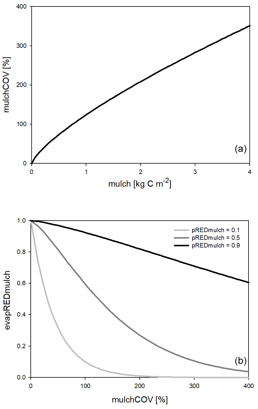
Figure 2Surface coverage as a function of the amount of surface residue or mulch (a) and the evaporation reduction factor (evapREDmulch) as a function of mulch coverage (b) using different mulch-specific soil parameters (pREDmulch). See text for details.

Download

3.4 Effect of groundwater

Simulation of the groundwater effect was introduced in Biome-BGCMuSo v4.0 (Hidy et al., 2016), but the method has been significantly improved, and the new algorithm it is now available in Biome-BGCMuSo v6.2. In the recent model version there is an option to provide an additional input file with the daily values of the groundwater table depth (GWdepth in meters).

Groundwater may affect soil hydrological and plant physiological processes if the water table is closer to the root zone than the thickness of the capillary fringe (that is the region saturated from groundwater via the capillary effect). The thickness of the capillary fringe (CF in meters) is estimated using literature data and depends on the soil type (Johnson and Ettinger model; Tillman and Weaver, 2006). Groundwater table distance (GWdist in m) for a given layer is defined as the difference between GWdepth and the depth of the midpoint of the layer.

The layers completely below the groundwater table are assumed to be fully saturated. In the case of layers within the capillary fringe (GWdist<CF), the calculation of water balance changes: the FC rises, and thus the difference between saturation (SAT) and FC decreases, and the layer charges gradually until the increased FC value is reached. The FC rising effect of groundwater for the layers above the water table is calculated based on the ratio of the groundwater distance and the capillary fringe thickness, but only after the water contents of the layers below have reached their modified FC values. A detailed description of the groundwater effect can be found in Sect. S6 in the Supplement.

3.5 Soil moisture stress

In the original Biome-BGC model the effect of changing soil water content on photosynthesis and decomposition of soil organic matter is expressed in terms of soil water potential (Ψ). Instead of Ψ, the SWC is also widely used to calculate the limitation of stomatal conductance and decomposition. A practical advantage of using SWC as a factor in the stress function is that it is easier to measure in the field and the changes in the driving function are much smoother than in the case of Ψ. The disadvantage is that SWC is not comparable among different soil types (in contrast to Ψ).

The maximum of SWC is the saturation value; the minimum is the wilting point or the hygroscopic water depending on the type of simulated process. The novelty of Biome-BGCMuSo v6.2 is that the hygroscopic water, the wilting point, the field capacity, and the saturation values are calculated internally by the model based on the soil texture data, or they can be defined in the input file layer by layer.

In Biome-BGCMuSo v6.2 the so-called soil moisture stress index (SMSI) is calculated to represent overall soil stress conditions. SMSI is affected by the length of the drought event (SMSE: extent of soil stress) and the severity of the drought event (SMSL: length of soil stress), and it is aggravated by extreme temperature (extremT: effect of extreme heat). SMSI is equal to zero if no soil moisture limitation occurs and equal to 1 in the case of full soil moisture limitation. SMSI is used by the model for plant senescence calculations (presentation of plant-related processes is the subject of a forthcoming publication). The components of SMSI are explained in detail below.

The magnitude of soil moisture stress (SMSE) is calculated layer by layer based on SWC. Regarding soil moisture stress two different processes are distinguished: drought (i.e., low SWC close to or below WP) and anoxic conditions (i.e., after large precipitation events or in the presence of a high groundwater table; Bond-Lamberty et al., 2007). An important novelty of Biome-BGCMuSo v6.2 is the soil curvature parameter (q), which is introduced to provide a mechanism for soil-texture-dependent drought stress as it can affect the shape of the soil stress function (which means a possibility for a nonlinear ramp function):

where q is the curvature of the soil stress function, and ${\text{SWC}}_{\text{drought}}^i$ and ${\text{SWC}}_{\text{anoxic}}^i$ are critical SWC values for calculating soil stress.

In order to make the SWC values comparable between different soil types, ${\text{SWC}}_{\text{drought}}^i$ and ${\text{SWC}}_{\text{anoxic}}^i$ can be set in normalized form (such as in Eq. 4) as part of the ecophysiological parameterization of the model. More details about the adjustment of the critical SWC values can be found in Hidy et al. (2021).

The layer-specific soil moisture stress extent values are summed across the root zone using the relative quantity of roots in the layers (RPⁱ) as weighting factors to obtain the overall soil moisture stress extent (SMSE):

where nr is the number of soil layers in which roots can be found, RL is the actual length of roots, and RD is the rooting distribution parameter (ecophysiological parameter; see details in the user guide; Hidy et al., 2021). In the current model version SMSE can also affect the entire photosynthetic machinery by the introduction of an empirical parameter. This mechanism is responsible for accounting for the non-stomatal effect of drought on photosynthesis (details about this algorithm will be published in a separate paper). Since there is no mechanistic representation behind this empirical downregulation of photosynthesis, further tests are needed for the correct setting of this parameter preferentially using eddy covariance data.

The factor (SMSL) related to soil moisture stress length is the ratio of the critical soil moisture stress length (ecophysiological parameter) and the sum of the daily (1−SMSE) values. This cumulated value restarts if SMSE is equal to 1 (no stress). Extreme heat (extremT) is also considered and is taken into account in the final stress function (see above) by using a ramp function. Its parameterization thus requires the setting of two critical temperature limits that define the ramp function (set by the ecophysiological parameterization; see Hidy et al., 2021). Its characteristic temperature values can be set by parameterization (ecophysiological input file).

4.1 Soil–litter module

We made substantial changes in the soil biogeochemistry module of the Biome-BGC model. Previous model versions already offered solutions for multilayer simulations (Hidy et al., 2012, 2016), but some pools still inherited the single-layer logic of the original model. In the new model version all relevant soil processes are separated layer by layer, which is a major step forward.

Instead of defining a single litter, soil organic carbon (SOC), and nitrogen pool, we implemented separate carbon and nitrogen pools for each soil layer in the form of soil organic matter (SOM) and litter in Biome-BGCMuSo v6.2. The changes in the mass of the carbon and nitrogen pools are calculated layer by layer. Mortality fluxes (whole plant mortality, senescence, litterfall) of aboveground plant material are transferred into the litter pools of the topsoil layers (0–10 cm, layers 1–2). Mortality fluxes of belowground plant material are transferred into the corresponding soil layers based on their location within the root zone. Due to ploughing and leaching, carbon and nitrogen can also be relocated to deeper layers. The plant material turning into the litter compartment is divided between the different types of litter pools (labile, unshielded cellulose, shielded cellulose, and lignin) according to the parameterization. Litter and soil decomposition fluxes (carbon and nitrogen fluxes from litter to soil pools) are calculated layer by layer, depending on the actual temperature and SWC of the corresponding layers. Vertical mixing of soil organic matter between the soil layers (e.g., bioturbation) is not implemented in the current model version.

Figure 3 shows the most important simulated soil and litter processes. N fixation (Nf) is the N input from the atmosphere to soil layers in the root zone by microorganisms. The user can set its annual value as an input parameter. N deposition (Nd) is the N input from the atmosphere to the topsoil layers (see below). The user can set its annual value as a site-specific parameter in the initialization input file. Nitrogen deposition can be provided by annually varying values as well. Plant uptake (PU) is the absorption of mineral N by plants from the soil layers in the root zone. Mineralization (MI) is the release of plant-available nitrogen (flux from soil organic matter to mineralized nitrogen). Immobilization (IM) is the consumption of inorganic nitrogen by microorganisms (flux from mineralized nitrogen to soil organic matter). Nitrification (NI) is the biological oxidation of ammonium to nitrate through nitrifying bacteria. Denitrification (DN) is a microbial process whereby nitrate (${{\mathrm{NO}}_{\mathrm{3}}}^{-}$) is reduced and converted to nitrogen gas (N₂) through intermediate nitrogen oxide gases. Leaching (L) is the loss of water-soluble mineral nitrogen from the soil layers. If leaching occurs in the lowermost soil layer that means loss of N from the simulated system. Litterfall (LI) is the plant material transfer from plant compartments to litter. Decomposition is the C and N transfer from litter to soil pools and between soil pools. In the case of woody vegetation coarse woody debris (CWD) contains the woody plant material after litterfall before physical fragmentation. Litter has also four sub-pools based on composition: labile (L1), unshielded and shielded cellulose (L2, L3), and lignin (L4). Soil organic matter also has four sub-pools based on turnover rate: labile (S1), medium (S2), slow (S3), and passive (recalcitrant; S4). The soil-mineralized nitrogen pool contains the inorganic N forms of the soil: ammonium and nitrate.

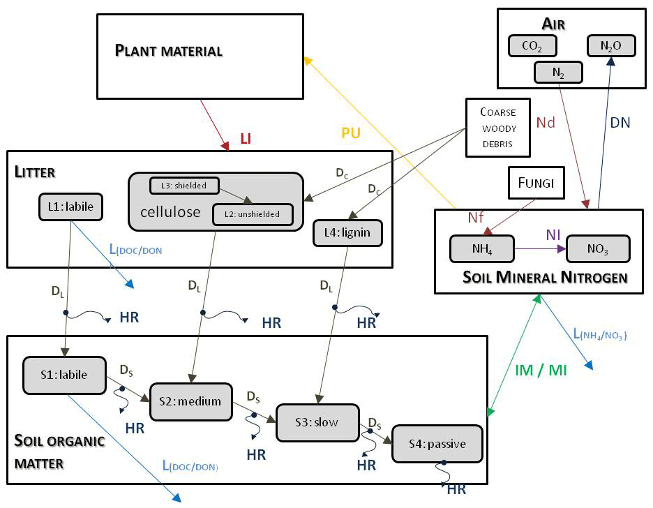
Figure 3Soil- and litter-related simulated carbon and nitrogen fluxes (arrows) as well as pools (rectangles) in Biome-BGCMuSo v6.2. HR: heterotrophic respiration, IM: immobilization, MI: mineralization, PU: plant uptake, LI: litterfall, NI: nitrification, D: decomposition (D_L: decomposition of litter, D_S: decomposition of SOM, D_C: fragmentation of coarse woody debris), L: leaching, Nf: nitrogen fixation, Nd: nitrogen deposition, DN: denitrification. L represents loss of C and N from the simulated system.

Download

4.2 Decomposition

In the decomposition module (i.e., converging cascade scheme; Thornton, 1998) the fluxes between litter and soil pools are calculated layer by layer. The potential fluxes are modified in the case of N limitation when the potential gross immobilization is greater than the potential gross mineralization.

To explain the decomposition processes implemented in Biome-BGCMuSo v6.2 the main carbon and nitrogen pools as well as fluxes between litter and soil organic and inorganic (mineralized) matter are presented in Fig. 4.

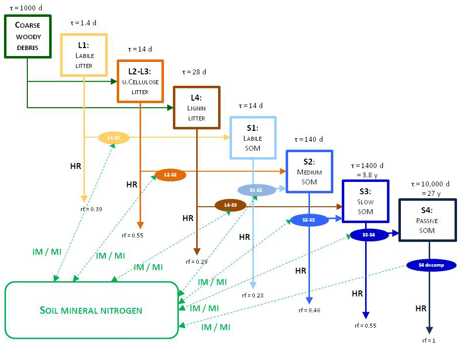
Figure 4Overview of the converging cascade model of litter and soil organic matter decomposition that is implemented in Biome-BGCMuSo v6.2. The notation rf represents the respiration fraction of the different transformation fluxes, and τ is the residence time (reciprocal of the rate constants, which is the turnover rate). IM/MI: immobilization and mineralization fluxes, HR: heterotrophic respiration. Note that both the respiration fraction and the turnover rate parameters can be adjusted through parameterization.

Download

In the original Biome-BGC and in previous Biome-BGCMuSo versions the C:N ratio (CN) of the soil pools was fixed in the model code. One of the new features in Biome-BGCMuSo v6.2 is that the CN of the passive soil pool (S4 in Fig. 4; recalcitrant soil organic matter) can be set by the user as a soil parameter. The CN of the other soil pools (labile, medium, and slow; S1, S2, and S3) is calculated based on the proportion of fixed CN values of the original Biome-BGC (${\text{CN}}_{\text{labile}}/{\text{CN}}_{\text{passive}}=\mathrm{1.2}$, ${\text{CN}}_{\text{medium}}/{\text{CN}}_{\text{passive}}=\mathrm{1.2}$, ${\text{CN}}_{\text{slow}}/{\text{CN}}_{\text{passive}}=\mathrm{1}$). Note that the CN of the donor and acceptor pools is used in decomposition calculations (see details in Sect. S7 in the Supplement), and as a result these parameters set the C:N ratio of the soil pools. The donor and acceptor pools can be seen in Figs. 3 and 4.

For the calculation of nitrogen mineralization, first respiration cost (respiration fraction) is estimated. Mineralization is then a function of the remaining part of the pool and its C:N ratio. The nitrogen mineralization fluxes of the SOM pools are functions of the potential rate constant (reciprocal of residence time) and the integrated response function that accounts for the impact of multiple environmental factors. The integrated response function of decomposition is a product of the response functions of depth, soil temperature, and SWC (F_r(d)_D, F_r(T)_D, F_r(SWC)_D; Fig. 5). Its detailed description can be found in Sect. S7. The dependence of the three different factors on depth, temperature, and SWC with default parameters is presented in Fig. 5.

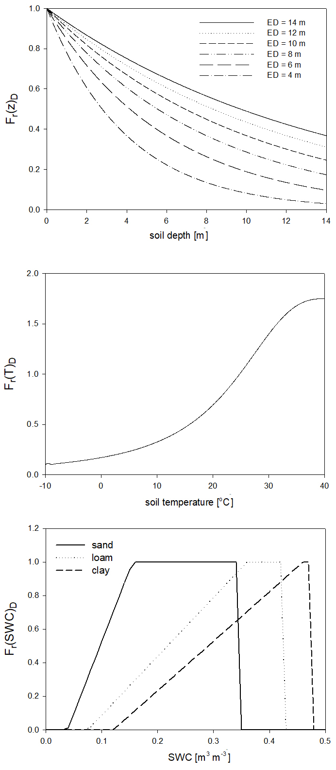
Figure 5The dependence of the individual factors that form the complex environmental response function of decomposition on depth (F_r(d)_D), temperature (F_r(T)_D), and SWC in the case of different soil types (F_r(SWC)_D). ED is the e-folding depth, which is one of the adjustable soil parameters of the model. For the definition of sand, silt, and clay see Fig. 1.

Download

4.3 Soil nitrogen processes

In Biome-BGCMuSo v6.2 separate ammonium (sNH4) and nitrate (sNO3) soil pools are implemented instead of a general mineralized nitrogen pool. This was a necessary step for the realistic representation of many internal processes like plant nitrogen uptake, nitrification, denitrification, consideration of the effect of different mineral and organic fertilizers, and N₂O emission.

It is important to introduce the availability concept that Biome-BGCMuSo uses and is associated with the ammonium and nitrate pools. We use the logic proposed by Thomas et al. (2013), which means that the plant has access only to a part of the given inorganic nitrogen pool. The unavailable part is buffered as it is associated with soil aggregates and is unavailable for plant uptake. The available part of ammonium is calculated based on the NH₄ mobile proportion (that is a soil parameter set to 10 % according to Thomas et al., 2013; Hidy et al., 2021) and the actual pool. The available part of nitrate is assumed to be 100 %.

The amount of ammonium and nitrate is determined layer by layer controlled by input and output fluxes (F, $\mathrm{kg}\mathrm{N}{\mathrm{m}}^{-\mathrm{2}}{\mathrm{d}}^{-\mathrm{1}}$) listed below:

where ${\text{IN}}_{\text{sNH4}}^i$ and ${\text{IN}}_{\text{sNO3}}^i$ are the input fluxes to the ammonium and nitrate pools, respectively; $L_{\text{sNH4}}^i$, $L_{\text{sNH4}}^{i-\mathrm{1}}$, $L_{\text{sNO3}}^i$, and $L_{\text{sNO3}}^{i-\mathrm{1}}$ represent the amount of leached mineralized ammonium and nitrate from a layer (i) or from the upper layer (i−1), respectively; ${\text{PU}}_{\text{sNH4}}^i$ and ${\text{PU}}_{\text{sNO3}}^i$ are the plant uptake fluxes of ammonium and nitrate, respectively; ${\text{IM}}_{\text{sNH4}}^i$ and ${\text{IM}}_{\text{sNO3}}^i$ are the immobilization fluxes of ammonium and nitrate, respectively; ${\text{MI}}_{\text{sNH4}}^i$ and ${\text{MI}}_{\text{sNO3}}^i$ are the mineralization fluxes of ammonium and nitrate, respectively; ${\text{NI}}_{\text{sNH4}}^i$ is the nitrification flux of ammonium; and ${\text{DN}}_{\text{sNO3}}^i$ is the denitrification flux of nitrate.

In the following subsections the different terms of the equations are described in detail.

Nitrification (NI Eqs. 6 and 7)

Nitrification is a function of the soil ammonium content, the net mineralization, and the response functions of temperature, soil pH, and SWC (F_r(pH)_NI, F_r(T)_NI, and F_r(SWC)_NI, respectively) based on the method of Parton et al. (2001) and Thomas et al. (2013). Its detailed mathematical description can be found in Sect. S8 in the Supplement. The response functions with proposed parameters are shown in Fig. 6.

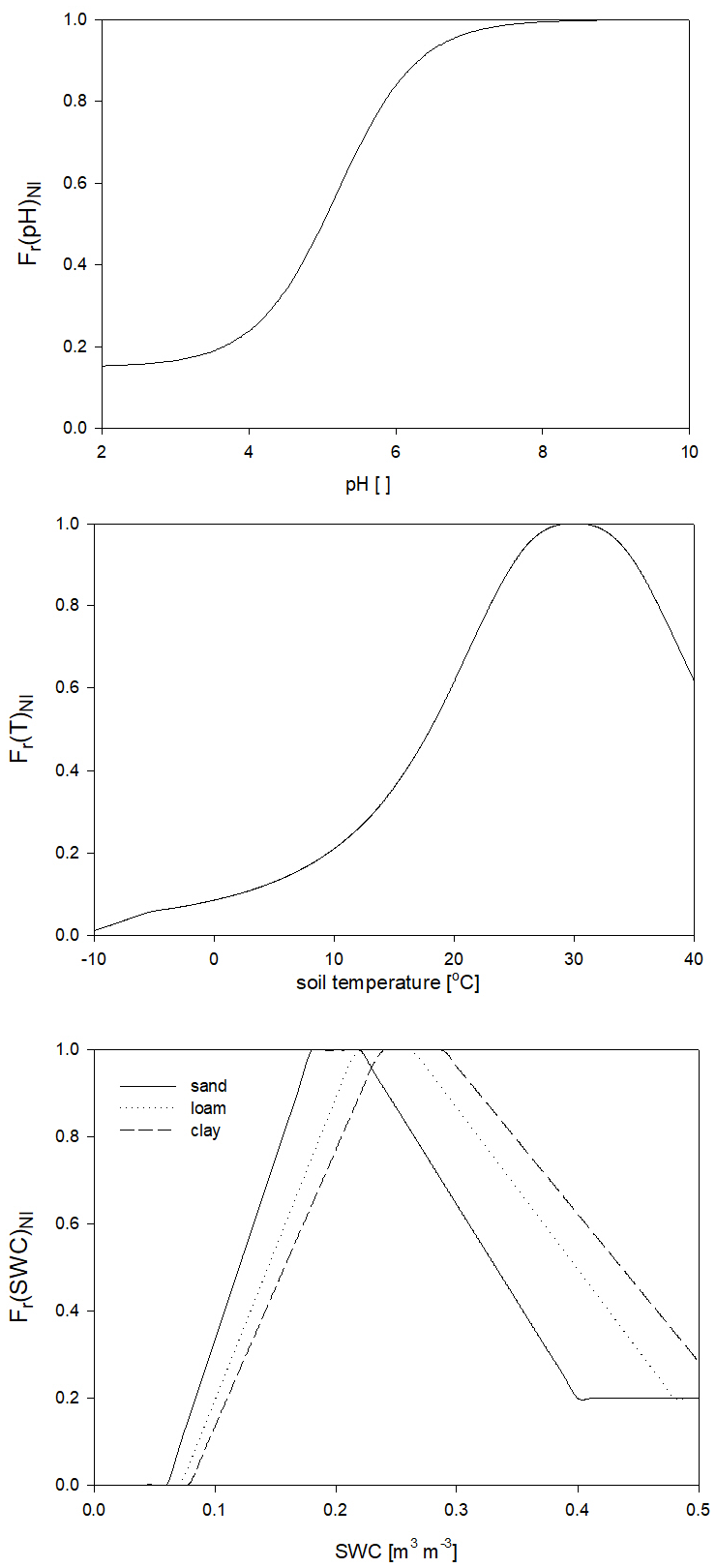
Figure 6The dependence of the individual factors of the environmental response function of nitrification on soil pH (F_r(pH)_NI), temperature (F_r(T)_NI), and SWC F_r(SWC)_NI in the case of different soil types. The pH and temperature response functions are independent of the soil texture.

Download

4.4 N₂O emission and N emission

During both nitrification and denitrification N₂O emission occurs, which (added to the N₂O flux originating from grazing processes if applicable) contributes to the total N₂O emission of the examined ecosystem.

In Biome-BGCMuSo v6.2 a fixed part (set by the coefficient of the N₂O emission of the nitrification input soil parameter; Hidy et al., 2021) of nitrification flux is lost as N₂O and not converted to NO₃.

During denitrification, nitrate is transformed into N₂ and N₂O gas depending on the environmental conditions: NO₃ availability, total soil respiration (proxy for microbial activity), SWC and pH. The denitrification-related ${\mathrm{N}}_{\mathrm{2}}/{\mathrm{N}}_{\mathrm{2}}\mathrm{O}$ ratio input soil parameter is used to represent the effect of the soil type on the ${\mathrm{N}}_{\mathrm{2}}/{\mathrm{N}}_{\mathrm{2}}\mathrm{O}$ ratio (del Grosso et al., 2000; Hidy et al., 2021). Detailed mathematical description of the algorithm can be found in Sect. S9 in the Supplement.

4.5 Leaching of dissolved matter

Leaching of nitrate, ammonium, and dissolved organic carbon and nitrogen (DOC and DON) content from the actual layer is calculated as the product of the concentration of the dissolved component in the soil water and the amount of water (drainage plus diffusion) leaving the given layer either downward or upward. The dissolved component (concentration) of organic carbon is calculated from the SOC pool contents and the corresponding fraction of the dissolved part of SOC soil parameters. The dissolved component of the organic nitrogen content of the given soil pool is calculated from the carbon content and the corresponding C:N ratio. The downward leaching is net loss from the actual layer and net gain for the next layer below; the upward flux is net loss for the actual layer and net gain for the next layer up. The downward leaching of the bottom active layer (ninth) is net loss for the system. The upward movement of dissolved substance from the passive (10th) layer is net gain for the system.

5.1 Evaluation of soil hydrological simulation

In order to evaluate the functioning of the new model version (and to compare simulation results made by the current and previously published model version), a case study is presented regarding soil water content and soil evaporation simulations. The results of a bare soil simulation (i.e., no plant is assumed to be present) are compared to observation data from a weighing lysimeter station installed at Martonvásár, Hungary ($\mathrm{47}{}^{\circ }{\mathrm{18}}^{\prime }{\mathrm{57.6}}^{\prime \prime }$ N, $\mathrm{18}{}^{\circ }{\mathrm{47}}^{\prime }{\mathrm{25.6}}^{\prime \prime }$ E), in 2017. The climate of the area is continental with a 30-year average temperature of 11.0 ^∘C (−1 ^∘C in January and 21.2 ^∘C in July) and annual rainfall of 548 mm based on data from the on-site weather station.

The station consists of 12 scientific lysimeter columns 2 m deep with 1 m diameter (Meter Group Inc., USA) and with soil temperature, SWC, and soil water potential sensors installed at 5, 10, 30, 50, 70, 100, and 150 cm depth. Observation data for 2020 from six columns without vegetation cover (i.e., bare soil) were used to validate the model.

Raw lysimeter observation data were processed using standard methods. Bare soil evaporation values were derived based on changes in the mass of the soil columns also considering the mass change in the drainage water. Additionally, experience has shown that wind speed is related to the high-frequency mass change in the soil column mass. To reduce noise, five-point (5 min) moving averages were used based on Marek et al. (2014). After quality control of the data, the corrected and smoothed lysimeter mass values were used for the calculations. SWC observations were averaged to daily resolution to match the time step of the model.

Observed local meteorology was used to drive the models for the year 2020. Soil physical model input parameters (field capacity, wilting point, bulk density, etc.) were determined in the laboratory using 100 cm³ undisturbed soil samples taken from various depths during the installation of the lysimeter station. Regarding other soil parameters the proposed values were used. A detailed description of the input soil parameters and their proposed values is presented in the user guide (Hidy et al., 2021).

In Fig. 7 the simulated and observed time series of soil evaporation are presented for Martonvásár for 2020. The figure shows that the soil evaporation simulation by v6.2 is more realistic than by v4.0. Biome-BGCMuSo v4.0 provides very low values during summer on some days, which is not in accordance with the observations. Biome-BGCMuSo v6.2 provides more realistic values during this time period.

Figure 7The simulated (blue line: v4.0; red line: v6.2) and observed (grey dots) daily soil evaporation values at Martonvásár during 2020. Vertical grey lines associated with the observations represent the standard deviation of the observations from six lysimeter columns. The improved model clearly outperforms the earlier version.

Download

In Fig. 8 the simulated and observed SWCs at 10 cm depth are presented with the daily sum of precipitation representing the bare soil simulation in Martonvásár for 2020. The soil water balance simulation seems to be realistic using v6.2, since the annual course captures the low and high end of the observed values. In contrast, Biome-BGCMuSo v4.0 underestimates the range of SWC and provides overestimations during the growing season (from spring to autumn). With a couple of exceptions, the simulated values using v6.2 fall into the uncertainty range of the measured values defined by the standard deviation of the six parallel measurements. This is not the case for the simulations with the 4.0 version.

Figure 8The simulated (blue line: v4.0; red line: v6.2) and observed (grey dots) soil water content values at 10 cm depth (right y axis) with the daily sums of precipitation (left axis; black columns) during 2020 at the Martonvásár lysimeter station. Vertical grey lines associated with the observations represent ± 1 standard deviation around the observations. The improved model clearly outperforms the earlier version in simulating soil water balance.

Download

Model performance was evaluated by quantitative measures such as the coefficient of determination (R²), mean absolute error (MAE), and mean signed error (MSE). In Fig. 9 the comparison of the simulated and observed daily evaporation is presented. Based on the performance indicators it is obvious that the simulation with the new model version (v6.2) is much closer to observations than the old version (v4.0). Biome-BGCMuSo v6.2 slightly underestimated the observations.

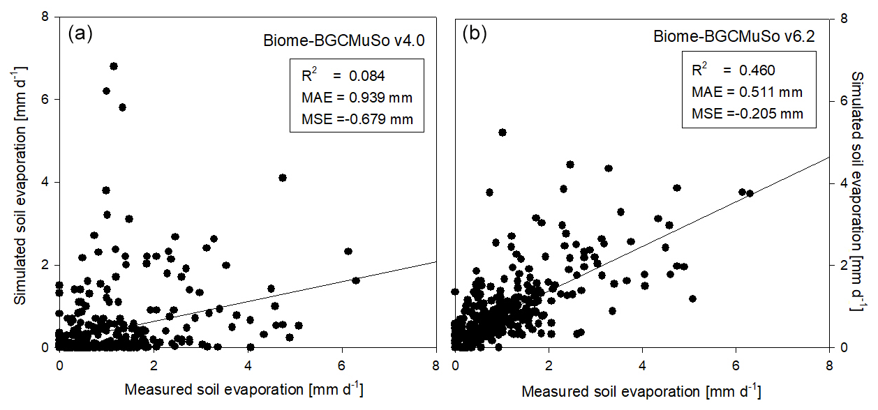
Figure 9Comparison of the simulated (a: v4.0; b: v6.2) and observed daily soil evaporation representing the means of measured data obtained from six weighing lysimeter columns with bare soil at Martonvásár in 2020. R², MAE, and MSE denote the coefficient of determination, mean absolute error, and mean signed error (bias) of the simulated values, respectively.

Download

In Fig. 10 the comparison of the simulated and observed daily SWC from the lysimeter experiment is presented. Based on the model evaluation it seems that the simulation with the new model version is much closer to observations than with old version (4.0). The results obtained from v4.0 are consistent with earlier findings about the incorrect representation of the annual SWC cycle (Hidy et al., 2016; Sándor et al., 2017).

Figure 10Comparison of the simulated (a: v4.0; b: v6.2) and observed daily SWC representing the means of measured data obtained from six weighing lysimeter columns with bare soil at Martonvásár in 2020. R², MAE, and MSE denote the coefficient of determination, mean absolute error, and mean signed error (bias) of the simulated values, respectively.

Download

A thorough validation of the improved model based on observed SWC and ET datasets from eddy covariance sites is planned to be published in an upcoming paper about the plant-related improvements.

5.2 Evaluation of the soil nitrogen balance module and the simulated soil respiration

Soil-related developments were evaluated with a case study focusing on topsoil nitrate content, soil N₂O efflux, and soil respiration.

Experimental data were collected in a long-term fertilization experiment that was set up in 1959 at Martonvásár, Hungary ($\mathrm{47}{}^{\circ }{\mathrm{18}}^{\prime }{\mathrm{41}}^{\prime \prime }$ N, $\mathrm{18}{}^{\circ }{\mathrm{46}}^{\prime }{\mathrm{50}}^{\prime \prime }$ E). According to the FAO-WRB classification system (IUSS Working Group, 2015), the soil is a Haplic Chernozem, with 51.4 % sand, 34 % silt, and 14.6 % clay content. Bulk density is 1.47 g cm⁻³, pH(H₂O) is 7.3, CaCO₃ content is 0 %–1 %, and the mean soil organic matter content in the topsoil is 3.2 %. The plant-available macronutrient supply in the soil was poor for phosphorus and medium to good for potassium based on the ProPlanta plant nutrition advisory system (Fodor et al., 2011). In the long-term fertilization experiment the treatments were arranged in a random block design with 6 m×8 m plots in four replicates. Eight different treatments were set up: control (zero artificial fertilizer applied), only N, only P, NPK – with farmyard manure, absolute control (zero nutrient supply), only N, only P, and NPK – without farmyard manure. The crop in the 4-year fertilizer cycles was maize in the first and second years and winter wheat in the third and fourth years. Here we used data from the absolute control and from the farmyard manure (FYM) treatments only. FYM was applied once every 4 years at a rate of 35 t ha⁻¹ in autumn.

Topsoil nitrate content was measured during 2017, 2018, and 2020 on a few occasions by wet chemical reactions using a stream distillation method after KCl extraction of soil samples (Hungarian Standards Institution MSZ 20135:1999; Akhtar et al., 2011).

Dynamic-chamber-based soil N₂O efflux observations were available from 2020 and 2021. The N₂O efflux measurements with a gas incubation time of 10 min were performed by using a Picarro G2508 (Picarro, USA) cavity ring-down spectrometer (Christiansen et al., 2015; Zhen et al., 2021). The cylinder-shaped transparent gas incubation chamber was 16.5 cm in diameter, and its height was 30 cm. N₂O flux measurements were executed in six replicates per treatment on a biweekly (2020) and precipitation-event-related (2021) basis. Soil respiration was measured with the same Picarro gas analyzer. Sampling numbers and points were identical to those of the N₂O efflux measurements. CO₂ and N₂O effluxes were calculated by a linear equation (Widen and Lindroth, 2003) based on gas concentration data.

For the simulations we used a maize parameterization from previous studies (Fodor et al., 2021). A winter wheat parameterization was constructed based on a country-scale optimization using the AgroMo software package (https://github.com/hollorol/AgroMo, last access: November 2021) and the NUTS 3 level long-term (1991–2020) yield database of the Hungarian Central Statistical Office. For nitrogen-cycle-related parameters we mainly used the values presented in the user guide (Hidy et al., 2021). Two soil parameters were adjusted (coefficient of N₂O emission for nitrification and ${\mathrm{N}}_{\mathrm{2}}/{\mathrm{N}}_{\mathrm{2}}\mathrm{O}$ ratio multiplier for denitrification-related N gas flux; Del Grosso et al., 2000; Parton et al., 2001; Thomas et al., 2013; Hidy et al., 2021) to match the simulated N₂O efflux to the observations.

Figure 11 shows the comparison of the simulated and observed NO₃ content of the topsoil for the two selected treatments. The results indicate that the model underestimates the topsoil NO₃ content in the case of both C and FYM (bias is −2.3 and −2.4 ppm, respectively) treatments, but the simulation error is in an acceptable range (NRMSE is 45.5 % and 37.6 % for C and FYM, respectively).

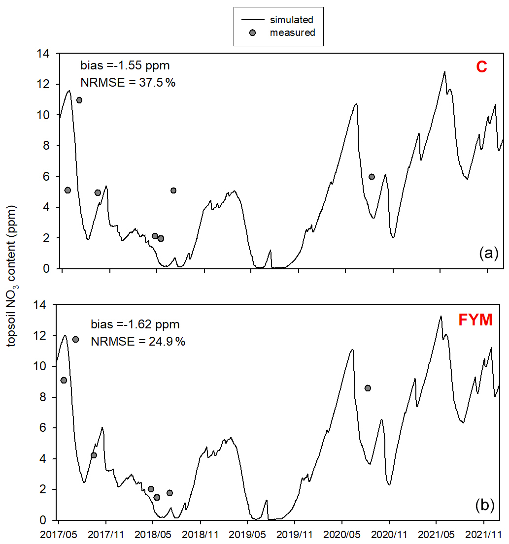
Figure 11Comparison of the simulated and observed NO₃ content of the topsoil for the absolute control (C; a) and for the farmyard manure (FYM; b) treatment between May 2017 and November 2021 at Martonvásár.

Download

Figure 12 shows the comparison of the observed and simulated N₂O efflux for the 2020–2021 time period. Measurement uncertainties are also indicated. Note that the uncertainty of the observations (e.g., due to spatial heterogeneity and sample number, soil disturbance, improper chamber design, methods of sample analysis) is remarkable due to known features of the chamber technique (Chadwick et al., 2014; Pavelka et al., 2018). The model captured more of the magnitude of N₂O efflux peaks and less of their timing. Overall the model underestimated the observed values in both cases (bias is −0.13 and −0.1 $\mathrm{mg}\mathrm{N}{\mathrm{m}}^{-\mathrm{2}}{\mathrm{d}}^{-\mathrm{1}}$ for C and FYM, respectively), with NRMSE of 32.4 % and 37.6 % for C and FYM, respectively.

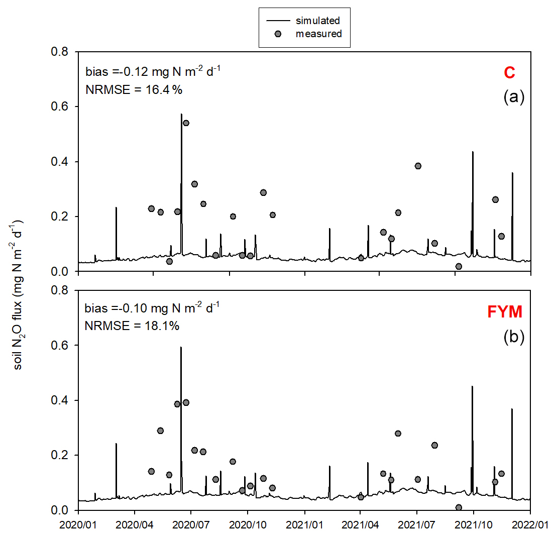
Figure 12Comparison of the simulated and observed soil N₂O efflux for two treatments: absolute control (C; a) and application of farmyard manure (FYM; b) between January 2020 and December 2021 at Martonvásár. Whiskers indicate the uncertainty (± 1 standard deviation) of the measurements.

Download

Figure 13 presents the comparison of the observed and simulated soil respiration for the same time period as for the soil N₂O efflux. Observation uncertainty is indicated that represents 1 standard deviation of the replicates. The model mostly captured the magnitude and variability of soil respiration flux. The model overestimated the observed values in both cases with bias of 0.17 and 0.04 $\mathrm{g}\mathrm{C}{\mathrm{m}}^{-\mathrm{2}}{\mathrm{d}}^{-\mathrm{1}}$ for C and FYM, respectively. The NRMSE is 34.1 % and 40.1 % for C and FYM, respectively. It is interesting to note that the observations and the simulations are particularly different after harvest time in both years (i.e., beginning of October). The simulated respiration has peaks corresponding to harvest when the amount of litter sharply increases due to the by-products left behind (decomposition of residues left on the site after harvest is accounted for in the model). The chamber-based CO₂ efflux data did not really show similar peaks, likely because of methodological issues (litter is removed from the soil surface before placing of the chambers).

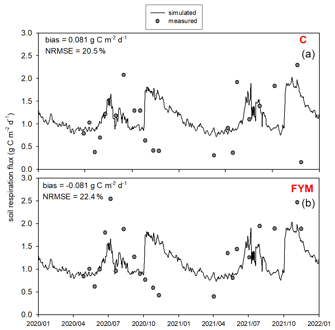
Figure 13Comparison of the simulated and observed soil respiration flux for two treatments: absolute control (C; a) and application of farmyard manure (FYM; b) between January 2020 and December 2021 at Martonvásár. Whiskers indicate the uncertainty (± 1 standard deviation) of the measurements.

Download

Overall, the model provided nitrate content, N₂O emission, and soil respiration simulation results that are consistent with the observations. The model was capable of estimating the observed values with comparable efficiency reported in similar studies (Gabrielle et al., 2002; Andrews et al., 2020).

5.3 Sensitivity analysis and optimization of the soil biogeochemistry scheme

Here we present another case study that provides insight into the functioning of the converging cascade (decomposition) scheme that is implemented in Biome-BGCMuSo v6.2. A large-scale in silico experiment is also presented, the main aim of which was to perform model self-initialization (i.e., spin-up) at country scale (for the entire area of Hungary) with the resulting soil organic matter pools expected to be consistent with the observations.

The observation-based, gridded, multilayer SOC database of Hungary (DOSoReMI database; Pásztor et al., 2020; see Figs. S3–S4 in the Supplement) and the FORESEE meteorological database (Kern et al., 2016) were used for the sensitivity analysis of the soil scheme as well as for optimizing the most important soil parameters when the model was calibrated to the observation-based SOC values. As a first step, the area of the country was divided into 1104 grid cells (regular grid with 0.1^∘ by 0.1^∘ resolution, corresponding to approximately 10 km resolution). The 1104 grid cells of the DOSoReMI database were grouped based on their dominant land use type (cropland, grassland, or forest based on the CORINE-2018 database; EEA, 2021; Figs. S1–S2 in the Supplement) as well as the soil texture class (12 classes according to the USDA system; USDA, 1987) and SOC content (high and low; high is greater than the group mean, while low is less than the mean) of the topsoil (0–30 cm layer). As some of the theoretically possible 72 groups had no members (e.g., there is no soil in Hungary with sandy–clay texture) soils of the 1104 grid cells were categorized into 51 groups. For each group one single cell (so-called representative cell) was selected based on the topsoil SOC content. The representative cell was the one with the smallest absolute deviation from the group mean SOC content (land use maps for Hungary are presented in Sect. S10 in the Supplement: Figs. S1–S2).

The grassland ecophysiological parameterization without management was used in the spin-up phase to initialize SOC pools for croplands. For the transient phase, the cropland parameterization was used with fertilization, ploughing, planting, and harvest settings. In the case of grasslands, a grassland parameterization was used during both the spin-up and transient phases, and in the transient phase mowing was assumed once a year. In the case of forests a generic deciduous broadleaf forest parameterization was used for both the spin-up and transient phases with thinning in the latter phase. For our parameterization presented in the MS the generic, plant-functional-type-specific ecophysiological parameter sets published by White et al. (2000) served as starting points. These Biome-BGCMuSo-specific parameter sets are available at the website of the model¹.

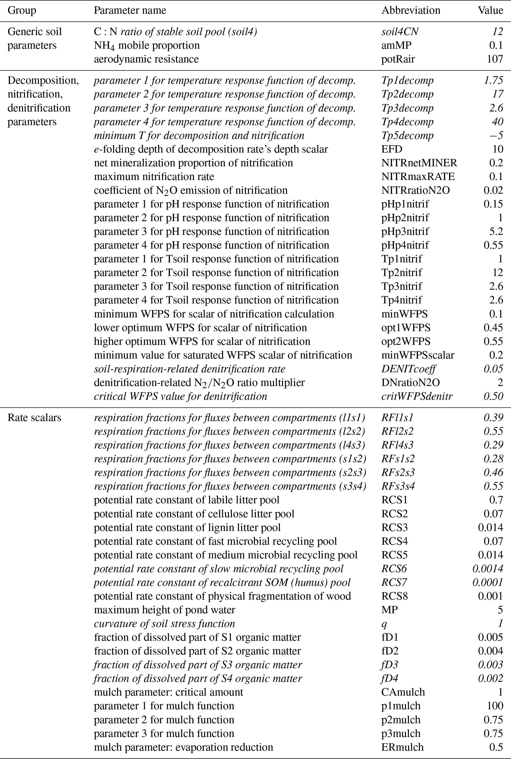
Soil parameters in Biome-BGCMuSo v6.2 were classified into six groups: (1) 4 generic soil parameters; (2) 24 parameters related to decomposition, nitrification, and denitrification; (3) 14 rate scalars for the converging (decomposition) cascade scheme; (4) 19 soil-moisture-related parameters; (5) 7 methane-related parameters; and (6) 11 soil composition and characteristic values (can be set layer by layer). A detailed description and proposed value of each soil parameters can be found in the user guide (Hidy et al., 2021).

As methane simulation was not the subject of the present case study we neglected the related parameters. Regarding the soil composition and characteristic values we used the DOSoReMI database (Pásztor et al., 2020). From the remaining 61 parameters, soil depth, runoff curve number, and the three soil-moisture-related parameters (tipping bucket method) were not included in the analysis. The groundwater module was switched off in this case (no groundwater is assumed) and the related parameters were not studied. The remaining 53 parameters were used in the sensitivity analysis and are listed in Table 1.

Table 1Soil parameters of Biome-BGCMuSo v6.2 (referring to SOC simulation) that were used during the sensitivity analysis. The “Value” column shows the originally proposed values (Hidy et al., 2021). See Fig. 4 for an explanation of the compartment names. The parameters that were included in the second phase of the sensitivity analysis are marked with italics (see text).

Download Print Version | Download XLSX

As a first step sensitivity analysis was carried out for the selected 53 soil parameters by running the Biome-BGCMuSo v6.2 model in spin-up mode until a quasi-equilibrium in the total SOC was reached (that is the usual logic of the spin-up run). The model was run for each representative cell 2000 times with varying model parameters using the Monte Carlo method. All model parameters were varied randomly within the ±10 % range of their initial values that were inherited from the Biome-BGC model or were set according to the literature. The least square linearization (LSL) method (Verbeeck et al., 2006) was used for dividing output uncertainty into its input-parameter-related variability. As a result of the LSL method, the total variance of the model output and the sensitivity coefficient of each parameter can be determined. Sensitivity coefficients show the percent of total variance for which the given parameter is responsible.

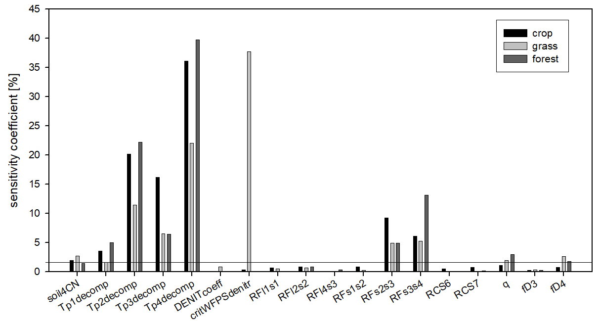
Figure 14The sensitivity coefficients of the soil parameters as the result of the sensitivity analysis. Black columns refer to the crop, light grey to the grass, and dark grey to the forest simulations. The sensitivity coefficients are calculated as the mean pixel-level sensitivity coefficient for the given land use type. The horizontal line indicates the 5 % threshold that was used to select the final parameter set for optimization.

Download

In order to simplify the workflow and decrease the degree of freedom another sensitivity analysis was performed. In this second step, the sensitive parameters (sensitivity coefficient >1 % for at least one land use type; a total of 18 parameters) were used in the following sensitivity analysis with 6000 iteration steps. These 18 parameters are marked with italics in Table 1.

Figure 14 shows the summary of the second sensitivity analysis wherein the overall importance of the parameters is calculated as the mean of all selected pixels in a given land use category. It can be seen in Fig. 4 that from the 18 parameters (selected during the first phase), the soil carbon ratio of the recalcitrant pool (soil4CN), the temperature dependence parameters of the decomposition function (Tp1decomp, Tp2decomp, Tp3decomp, Tp4_decomp), the respiration fraction of the S2–S3 and S3–S4 decomposition process (RFs2s3 and RFs3s4), the curvature of the soil stress function (q_soilstress), and the fraction of the dissolved part of S4 organic matter (fD4) are the most important for all land use types. Among the other parameters the critical WFPS of denitrification (critWFPSdentir) for grasslands has a remarkably high sensitivity (greater than 35 %). It means that in the case of grasslands the nitrogen availability seems to be an important limitation on primary production, probably because there are only natural sources of nitrogen (no fertilization is assumed here) and the rooting zone is shallower than in the case of forest, which involves limited mineralized N access. Thus, in the case of higher values of critical WFPS of denitrification, the simulated production of grassland (and therefore the final SOC) seems to be significantly underestimated.

The 10 selected soil-biogeochemistry-related parameters were optimized for each of the 51 groups separately using maximum likelihood estimation. For each group, the parameter set providing the smallest deviation between the simulated and observed values of the weighted average SOC content (weight factor of 5 for 0–30 cm and weight factor of 1 for 30–60 cm soil layers) was considered to be the final (optimized) model parameter set.

The differences of the simulated and observed SOC content for the 0–30 cm layer (SOC0-30) using the initial (Table 1) and final soil parameters (not shown here) are presented in Fig. 15. In the upper panel the signed relative error of SOC0-30 simulation before optimization can be seen, while in the lower panel the signed relative error of SOC0-30 simulation after optimization can be seen. It is clearly visible that because of optimization the overestimation of the SOC0-30 simulation significantly decreased.

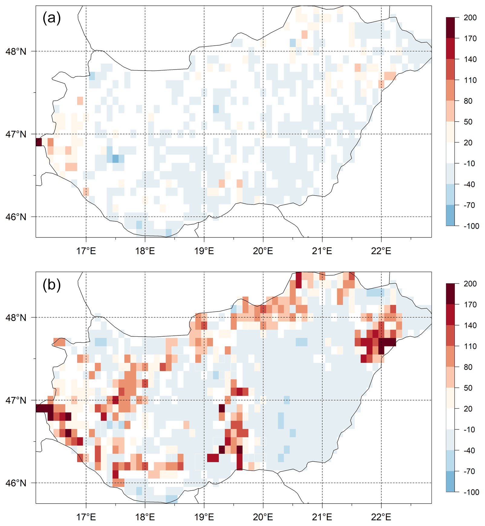
Figure 15Differences (expressed as signed relative error, %) between the simulated and observed SOC data for the 0–30 layer (SOC0-30) using the initial (a) and optimized (b) soil parameters. Visual comparison of the maps reveals the success of the optimization in terms of capturing the overall SOC for the whole country area.

Table 2Comparison of the internal processes simulated in Biome-BGC 4.1.1, Biome-BGCMuSo v4.0, and Biome-BGCMuSo v6.2.

Download Print Version | Download XLSX

We do not claim, of course, that the optimized parameters have universal value. Site history is neglected during the spin-up simulations, and we use many simplifications like disregarding land use change and present-day ecophysiological parameterization. In this sense, the optimized parameter set can best be considered a pragmatic solution to provide initial conditions (equilibrium SOC pools) for the model at country scale consistent with the observations.