2.1 Runoff-generation scheme in ELM v1

The ELM v1(hereafter, v1 is omitted) was developed based on the Community Land Model 4.5 (CLM4.5; Oleson et al., 2013) to understand the water availability and water cycle extremes (Leung et al., 2020). The new physical processes added in ELM to better represent the terrestrial water cycle include a variably saturated flow model (Bisht et al., 2018), a soil erosion model (Tan et al., 2020), dynamic roots (Drewniak, 2019), and a two-way coupled irrigation scheme (Zhou et al., 2020). The runoff generation in ELM is based on the simple TOPMODEL-based runoff parameterization (SIMTOP; Niu et al., 2005) in which the total runoff (R_total) consists of the following three components: surface runoff (R_over; e.g., saturation excess runoff), surface water runoff (R_h2osfc; e.g., surface water drainage from depressions/wetlands), and subsurface runoff (R_drai), as seen in the following:

A fraction of the flux of water reaching the soil surface (q_liq) generates surface runoff, and the fraction is determined by the saturation fraction (f_sat) of the grid cell as follows:

where f_max represents the maximum saturation fraction for a given grid cell that is calculated with high-resolution compound topographic indices, f_over is a decay factor, and z_∇ is the water table depth.

ELM includes surface water storage to represent inland/wetland surface water dynamics (Ekici et al., 2019). When the surface water storage is fully filled, surface water runoff is generated as follows:

where k_h2osfc represents the linear storage coefficient, f_connected is the interconnected fraction of the inundated areas, W_sfc is the mass of surface water, W_c is the mass of surface water when the storage is full, and Δt is the model time step. W_sfc is formulated as follows:

where erf represents the error function, d is the height of the surface water relative to the cell averaged elevation, and σ_micro is the standard deviation of the microtopographic distribution that characterizes subgrid elevation variation. Given the surface water height from the previous equation, the surface water fraction (f_h2osfc) of a cell is estimated with the following:

The inundation areas are assumed to be randomly distributed within the grid cell, and the interconnected fraction of the inundated areas can be estimated based on percolation theory, as follows:

where f_c is the threshold below which the inundated areas are not connected, and μ is a scaling exponent. The default parameter values in ELM of f_c and μ are 0.4 and 0.14 for all the global cells, respectively.

The subsurface runoff is parameterized as an exponential function of water table depth and includes an ice impedance factor (Θ_ice) to account for the reduction in the bottom drainage when ice is present in the soil (Swenson et al., 2012), as follows:

where q_drai,max is the maximum drainage rate, f_drai is the decay factor, $\frac{{\mathit{\theta }}_{\mathrm{ice}}}{{\mathit{\theta }}_{\mathrm{sat}}}$ represents the ice-filled fraction of the pore space for the soil under the water table, and Ω is an adjustable parameter.

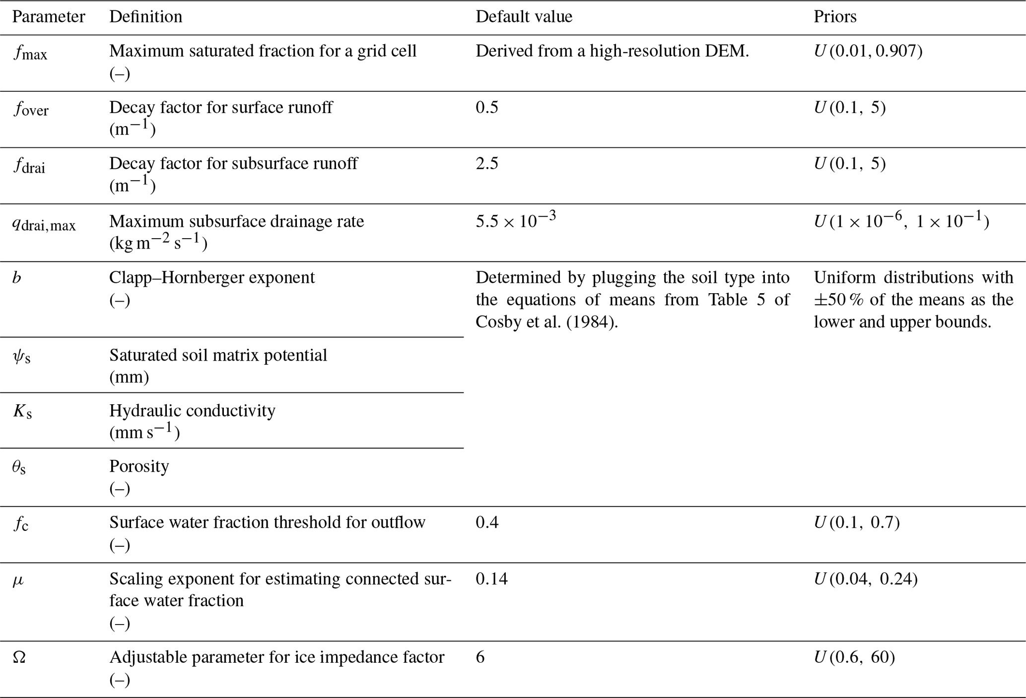
We follow the work of Huang et al. (2013) in selecting uncertain parameters and their corresponding ranges (Table 1). There are three additional parameters included in this study for surface water storage drainage and impacts of ice to subsurface runoff and soil water dynamics, which represent new features in ELM compared to CLM4.0 used in Huang et al. (2013). All the parameter prior distributions are assumed to be a uniform distribution.

Table 1Uncertain parameters' information. Note: DEM is for digital elevation model.

Download Print Version | Download XLSX

2.2 Model configuration

We ran ELM globally at a spatial resolution of 0.5^∘ × 0.5^∘, driven by the Global Soil Wetness Project forcing dataset (GSWP3v1) from 1991 to 2010, featuring 3 h, 0.5^∘ × 0.5^∘ global atmosphere forcing. GSWP3v1 has been dynamically downscaled and bias corrected based on the reanalysis data of Compo et al. (2011). The default configuration of ELM was used with a 30 min time step. With the default configuration, the hydrologic representations of ELM are the same as those in CLM4.5, as new model features such as the variably saturated flow model and subgrid topography are not included. Except the uncertain parameters listed in Table 1, the default values of all other ELM parameters were used in this study.

3.1 Polynomial chaos expansion

Let M denote a physical model (e.g., ELM) with uncertain parameters X, where $\mathbf{X}=[X_{\mathrm{1}},X_{\mathrm{2}},\mathrm{\dots },X_D]$, and D represents the total number of uncertain parameters. In this study, the uncertain parameters X are listed in Table 1 and D is 11. A scalar quantity of interest (QoI), $\widehat{y}$ (e.g., runoff at a specified time from a specified location), obtained using a sample of random parameters, x, can be expressed as a polynomial expansion, as follows:

where Ψ_α is a polynomial, and c_α is the corresponding coefficient. In practice, x is scaled to [−1, 1] from the original uncertainty input range. The polynomial expansion in Eq. (10) is written, with respect to multivariate orthogonal polynomials, as follows:

where ${\mathrm{\Psi }}_{{\mathit{\alpha }}_i}\left(x_i\right)$ is a univariate polynomial, whose form is associated with the prior distribution of uncertain input variable X_i (e.g., Legendre polynomials are used when the input variable follows a uniform distribution), and α_i is a member of the multi-index $\mathit{\alpha }=\left[{\mathit{\alpha }}_{\mathrm{1}},{\mathit{\alpha }}_{\mathrm{2}},\mathrm{\dots },{\mathit{\alpha }}_D\right]$, which represents the degrees of the univariate polynomial terms. Readers should refer to Dwelle et al. (2019) for details about the selection of polynomial terms and an illustration of how the multi-index is used to construct a PCE-based surrogate. In practice, Eq. (11) is approximated with a truncated PCE by only selecting terms with a total degree of polynomials smaller than a certain value p (Xiu and Karniadakis, 2002; Lin and Karniadakis, 2009). This leads to a finite set $A_p=(\mathit{\alpha }:{\sum }_{i=\mathrm{1}}^D{\mathit{\alpha }}_i\le p)$ for the multi-index α to take the following:

where j represents the counter-index of any possible multi-index α in A_p in a predefined order (see details in Appendix B of Dwelle et al., 2019). The coefficients (c_j) for the P+1 polynomial bases are computed using training simulations of M(x) (e.g., ELM) to construct the truncated PCE approximation in Eq. (12). The number of the polynomial basis is determined by both the input dimension D and the total degree for truncation p (Xiu and Karniadakis, 2002) is as follows:

The value P increases rapidly as the number of uncertainty input variables increases. For example, 11 uncertain parameters (e.g., D=11) with a truncated PCE order of p=4 lead to 1365 coefficients to solve in Eq. (12). It is computationally prohibitive to run 1365 global ELM simulations, so we adopted the BCS method of Sargsyan et al. (2014) that requires a much smaller number of ELM simulations to construct a PCE-based surrogate. The BCS method computes only a sparse set of c_j to construct the surrogate of a form given by Eq. (12) because not all Ψ_j(x) are relevant for the given QoI (Sargsyan et al., 2014).

3.2 Global sensitivity analysis

In this study, we performed variance-based, global sensitivity analysis using Sobol' indices (Sobol', 2001). For a PCE-based surrogate model, the main Sobol' index, S_i, for the uncertain parameter X_i can be estimated as follows:

where Π_i denotes all the indices of polynomial basis terms in Eq. (12) that only involve parameter X_i, and ||Ψ_j|| is the norm of the polynomial Ψ_j(x). The main Sobol' index S_i can be interpreted as the fraction of variance in the output that is associated with the uncertainty model parameter X_i only when other parameters are fixed at constant values. Similarly, one can estimate the Sobol' index for any pair of parameters X_i and $X_{i^{\prime }}$ to represent parameter interaction sensitivity with the coefficients c_j (Sargsyan et al., 2014).

3.3 Parameter inference

Parameter inference is used to determine a set of model parameters that reduces the error between observation and model prediction. The model inverse problem can be solved with the Bayes' theorem, as follows:

where p(X|y) is the posterior distribution of parameter X given observation y, L(y|X) is the likelihood function, p(X) represents the prior distribution of X, and p(y) is merely a normalizing constant for the purposes of parameter calibration. The discrepancy between the model and observations, $\mathit{ϵ}=\mathit{y}-M\left(\mathbf{X}\right)$, should be included in the likelihood function. It is common to assume the error term (e.g., ϵ) follows a Gaussian distribution with a vanishing mean:

where N is the number of observations used to infer the parameters (e.g., time series of monthly runoff), and the standard deviation, σ, can be inferred from the data (see Sect. 3.4). Then, the likelihood function can be written as follows:

The logarithm of Eq. (17) leads to the least squares objective function that is used for deterministic parameter estimation in practice (Sargsyan et al., 2015), as follows:

The posterior distribution in Eq. (18) is difficult to compute in practice; hence, we estimate it through samples obtained by the Markov Chain Monte Carlo (MCMC) method. Specifically, 1000 iterations are used as the burn-in period in this study, and the sampling of the posterior distribution is saved every 10 iterations. We run MCMC for 10 000 steps, resulting in 1800 samples to construct the posterior distribution. We have employed adaptive MCMC method of Haario et al. (2001), in which the parameter space is searched according to proposal steps with a covariance that is updated spontaneously.

3.4 Quantity of interest

In this study, the physical model M and the QoI $\widehat{y}$ correspond to ELM and runoff, respectively. The development of a surrogate model for the simulated runoff for each grid cell for each month of a 20-year simulation would require 240 (= 12 months × 20 years) PCE-based surrogates. Although developing a PCE-based surrogate is not expensive, it is computationally expensive to train 240 PCEs for each of the 70 302 grid cells in the global domain. The parameter inference process for 240 PCEs for each grid cell will further increase the computational cost. We reduce the number of QoIs by training the surrogate model for the root mean square error (RMSE) between the simulated runoff and observations instead of training the surrogate model to predict monthly runoff. The RMSE is given as follows:

where $R_i^{\mathrm{sim}}$ and $R_i^{\mathrm{obs}}$ represent the grid-level simulated total runoff and observed total runoff, respectively, for ith month in the simulated period, and N represents the number of simulation months. Consequently, only one surrogate model is needed for each grid cell to quantify the performance of ELM in capturing the monthly runoff variation for a given uncertain parameter set. The selection of RMSE as QoI in constructing surrogate models significantly reduces the computational burden of the surrogates' construction and parameter inference. We performed ELM simulations using 200 parameter sets that were randomly sampled from the range specified in Table 1. A set of 175 ELM simulations were used for training the surrogate models, and the other 25 simulations were used for validating their performances. The performance of the PCE-based surrogate model can be affected by the truncated order (Dwelle et al., 2019). For each grid cell, we train the surrogate with $p=\mathrm{1},\mathrm{2},\mathrm{\dots },\mathrm{7}$ separately and picked the order that minimizes the relative norm 2 error (RE) of validation simulations as follows:

where RMSE${}_{\mathrm{val}}^{\mathrm{PC}}$ and RMSE${}_{\mathrm{val}}^M$ represent the PCE-simulated and ELM-simulated vector of RMSE of the 25 validation simulations, respectively. Then, the trained surrogate models, RMSE^PC, can be plugged into the likelihood function of Eq. (18) seamlessly, as follows:

The standard deviation of error between model simulated runoff and observation exhibits a significant monthly variation. To provide a reasonable value of σ, we further assume σ in Eq. (21) has a different meaning than that in Eq. (18) by taking RMSE as model simulation, and 0 as the target. Therefore, σ is approximated as the standard deviation of the difference between 0 and RMSEs, where each RMSE was calculated using simulated runoff and observation for a given training simulation. Our estimation of σ leads to a reasonable posterior (see Sect. 5.4), though other methods can also be used to estimate σ. We acknowledge that the value of σ may have an impact on the parameter posteriors, but investigating the sensitivity of σ on the posteriors is beyond the scope of this study.

3.5 Calibration procedure

In summary, the following procedures were implemented to determine the optimal parameter values and their joint probability distribution:

1. Run ELM with 200 parameter sets randomly sampled with the range specified in Table 1.

2. Construct PCE-based surrogate models to mimic the RMSE between the ELM and GRUN runoff dataset with 175 simulations and validate the performance of the surrogate models with the other 25 simulations.

3. Implement sensitivity analysis with the surrogate models to reduce parameter dimensionality for calibration by ignoring the parameters with negligible Sobol' index (e.g., less than 0.05).

4. Estimate the Bayesian posterior of the most sensitive parameters for each grid through MCMC process with the runoff dataset of Ghiggi et al. (2019a).

It has been shown that small surrogate error can result in significant deviation of the inferred parameter (Laloy and Jacques, 2019). To further search the optimal parameters and construct the runoff posterior uncertainty, we ran ELM simulations with additional 100 samples from the posteriors of the three most sensitive parameters for all global grid cells, and default values were used for less sensitive parameters.

The parameters with the minimum RMSE between simulations and reference runoff data from the 100 ELM simulations were determined as the optimal parameter value for each grid cell.

4.1 Observation-based runoff data

The 0.5^∘ × 0.5^∘ observation-based global runoff dataset (GRUN) dataset of Ghiggi et al. (2019a) was used in this study as the observation within the calibration framework for parameter inference. The GRUN dataset was generated from a trained random forest (RF) model (Breiman, 2001) that used precipitation and near-surface temperature to predict monthly runoff. The training runoff data were derived from the Global Streamflow Indices and Metadata Archive (GSIM; Gudmundsson et al., 2018; Do et al., 2018), and only the gauges with contributing area comparable to cell area of 0.5^∘ × 0.5^∘ were used. GSWP3 atmospheric forcing was used for training and reconstruction of the monthly global runoff.

4.2 Model benchmarks

The ILAMB package (Collier et al., 2018) was used to evaluate the simulated water and energy cycles from the calibrated ELM against various benchmarks. Specifically, a gridded energy flux data (FLUXCOM; Jung et al., 2019) that was generated by machine learning with flux tower measurements was used to evaluate latent and sensible heat fluxes, the Global Land Evaporation Amsterdam Model version 3 (GLEAMv3; Martens et al., 2017) product was used to evaluate global evapotranspiration (ET), and Gravity Recovery And Climate Experiment (GRACE; Kim et al., 2009) data were used to evaluate a terrestrial water storage anomaly (TWSA). Details about ILAMB can be found at https://www.ilamb.org (last access: 23 June 2021).

The Inter-Sectoral Impact Model Intercomparison Project (ISIMIP) archived simulations from multiple global hydrological models and land surface model forced by the same atmosphere forcings (Warszawski et al., 2014). We used 13 available models from the second-phase water sector (ISIMIP2a; Gosling et al., 2019) to provide a benchmark for the uncertainty of annual runoff magnitude and trend. Only the models in ISIMPI2a that were driven by the GSWP3 forcing without accounting for human activity impacts were selected here to be consistent with ELM's configuration.

4.3 Evaluation metrics

There were two metrics used to evaluate ELM's performance of simulating runoff at a monthly scale with calibrated parameters, including the Nash–Sutcliffe efficiency (NSE; Nash and Sutcliffe, 1970) and the Kling–Gupta efficiency (KGE; Gupta et al., 2009) which are computed as follows:

where $R_i^{\mathrm{sim}}$ and $R_i^{\mathrm{obs}}$ represent cell-level simulated total runoff and observed total runoff, respectively, for the ith month, μ_obs is the corresponding averaged observation, ρ is the correlation coefficient between simulation and observation, σ_sim is the standard deviation in simulations, σ_obs is the standard deviation in observations, and μ_sim is the simulation mean. Both NSE and KGE vary from −∞ to 1, and a perfect model performance is indicated by NSE = 1 and KGE = 1. NSE < 0 and KGE < −0.41 mean the simulations are worse estimates than the mean of observations, indicating a bad model performance (Knoben et al., 2019).

The sensitivity of runoff to precipitation is a critical aspect for runoff simulation evaluation, considering changes in precipitation will continue in the future (Trenberth, 2011). Therefore, we evaluated the sensitivity of runoff to the precipitation anomalies with the calibrated parameters. The sensitivity was quantified by the slope of linear regression (β) between runoff anomalies (ΔR) and precipitation anomalies (ΔP) as follows:

The interception ϵ ≈0, implies the mean runoff is related to mean precipitation.

We also evaluated the impacts of parameters on the runoff trend. Specifically, the magnitude of runoff trend was calculated with Sen's slope (Sen, 1968), which is nonparametric and not sensitive to the outliers. Then, Mann–Kendall test was used to determine if the trend is significant or not at confidence level α=0.05.

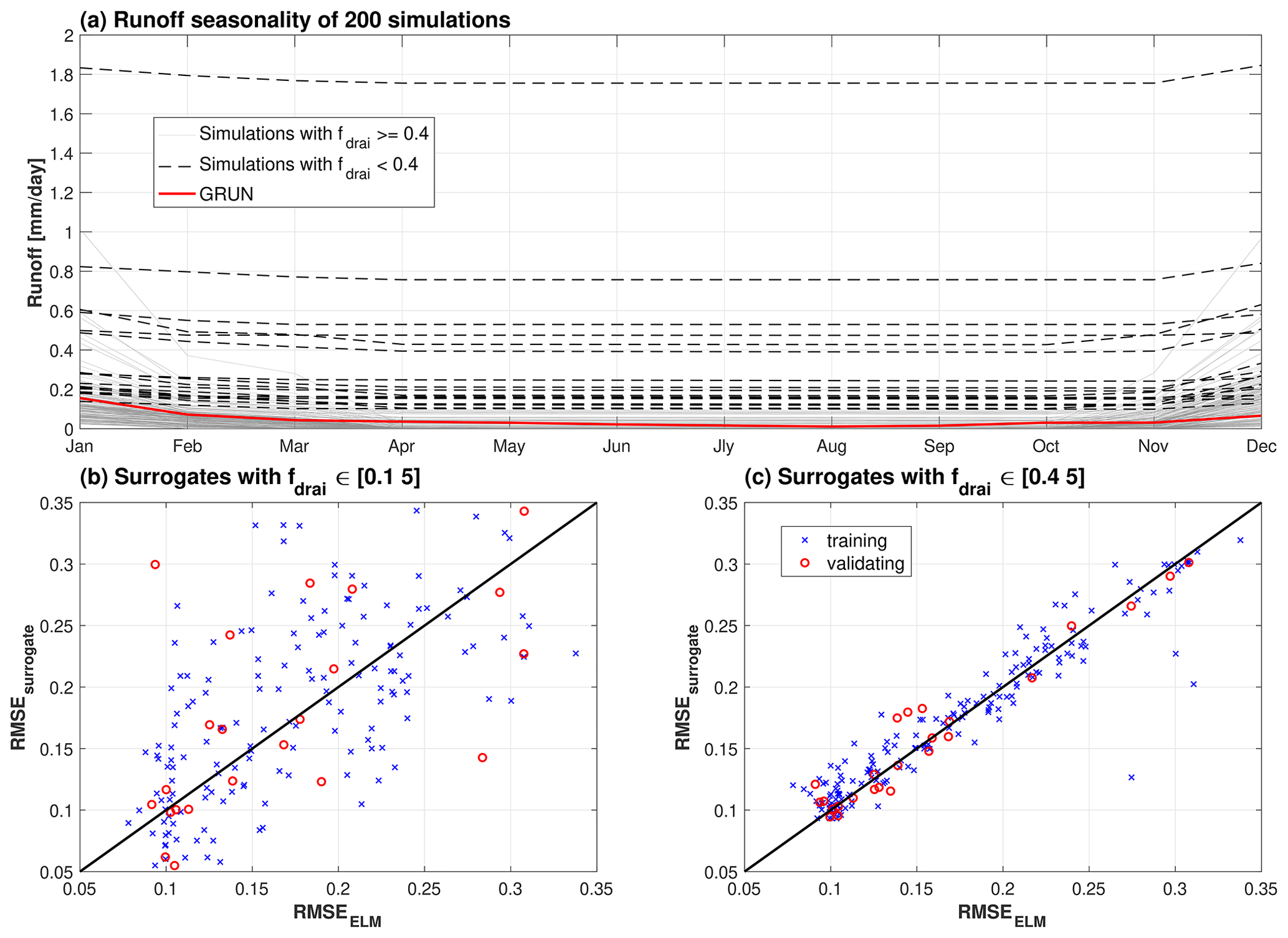
Figure 1Validation of surrogate performance for an example grid cell from an arid region. Panel (a) shows runoff seasonality from all 200 simulations with samples from parameter priors. Panel (b) shows the validation of the surrogate model trained with original ranges of f_drai given in Table 1 in the main text. Panel (c) shows the validation of the surrogate model trained with constrained f_drai.

Download

5.1 Refinement of f_drai for arid regions

The proposed prior for f_drai is not suitable for all the climate regions, such as the simulations with the full the range of f_drai defined in Table 1 results in unrealistic runoff for arid regions. For example, the simulated runoff from an example grid cell with f_drai<0.4 shows higher magnitudes and lower variabilities compared to simulations with f_drai≥0.4 (Fig. 1a). Lower f_drai can lead to unrealistically high subsurface runoff according to the exponential function of baseflow drainage (Eq. 8) for the arid regions, where the precipitation is not enough to maintain the water table at a reasonable level. Such simulations with f_drai<0.4 result in high nonlinearity in the simulated runoff, and hence, the PCE-based surrogate model cannot capture the model behaviors (Fig. 1b). The performance of surrogate models is improved by constraining the lower bound of f_drai to 0.4 (Fig. 1c). Therefore, f_drai is refined as [0.4, 5] for areas that are identified as arid climate in the Köppen climate classification (Fig. S1 in the Supplement), and [0.1, 5] is used in other regions.

5.2 Validation of surrogate models

The PCE-based surrogate models can mimic the variations in RMSE between ELM-simulated runoff and the GRUN runoff with the truncated order determined in Fig. S2. Specifically, the surrogate models exhibit good performance for the validation simulations with RE<0.1 for 70 % of the global domain (Fig. 2a). The global averaged RE of surrogate models for the validation simulations is around 0.1, with the largest error over the arid regions (Fig. 2b). While 41 % of the arid region shows an acceptable performance in the surrogate models when narrowing the range of f_drai with RE less than 0.15, the RE of other arid areas remain high (Fig. 2a). Additional simulations were performed to investigate if the lower performance of surrogate models for arid regions is due to insufficient number of training simulations. We randomly selected 20 grid cells from the arid region and ran 2000 ELM simulations with random samples from the parameter priors, as summarized in Table 1. The RE of surrogate models for the 20 grid cells remained large (e.g., RE > 0.2), even as the number of training simulations were increased (Fig. S3). Thus, the lower performance of surrogate models over the arid regions is not dependent on the number of training simulations.

Figure 2Relative norm 2 error of the surrogate models for the validation simulations. Panel (a) shows the spatial distribution of the errors, and panel (b) shows the average errors for the grid cells in each climate defined by Köppen climate classification.

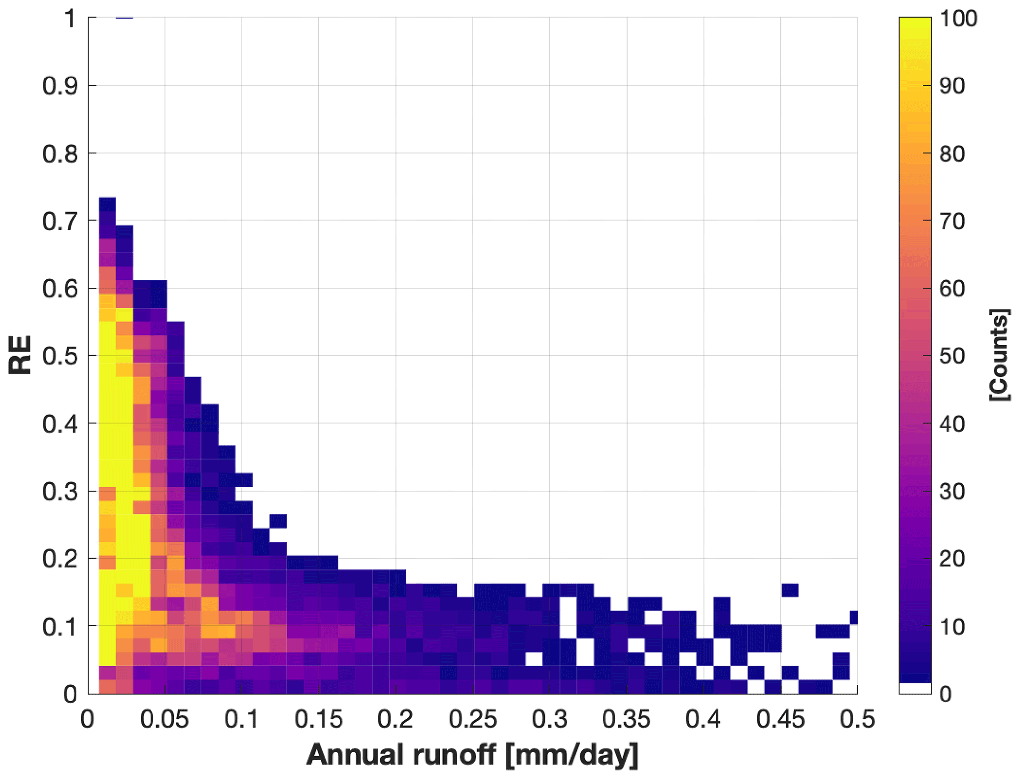
Figure 3Plot of relative norm 2 error (RE) of surrogate models for the validation simulations vs. averaged annual runoff magnitude with all the grid cells from the arid region.

Download

Most surrogate models with large RE are in extremely dry arid regions; for example, RE > 0.2 are mainly from grid cells with annual runoff <0.05 mm d⁻¹ (Fig. 3). The RE of surrogate models tends to decrease for areas with relatively higher annual runoff that are still from arid regions (annual runoff < 0.5 mm d⁻¹ in Fig. 3). However, the runoff uncertainty in extremely dry areas will have negligible impact on the global water cycle. Surrogate model with RE > 0.15 is considered as not sufficiently accurate, and such grid cells are excluded in the sensitivity analysis presented next.

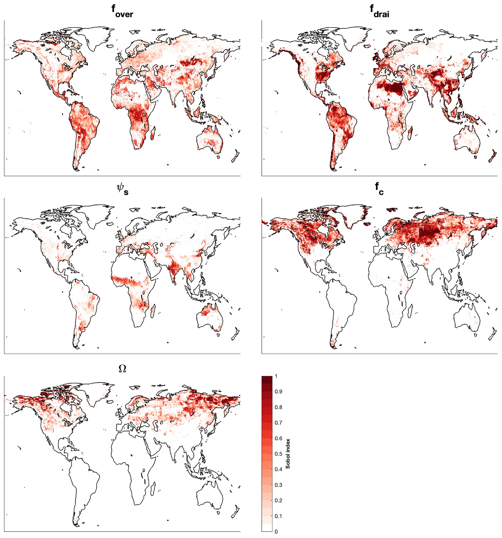
Figure 4Spatial distribution of the main Sobol' index for the sensitivity parameters.

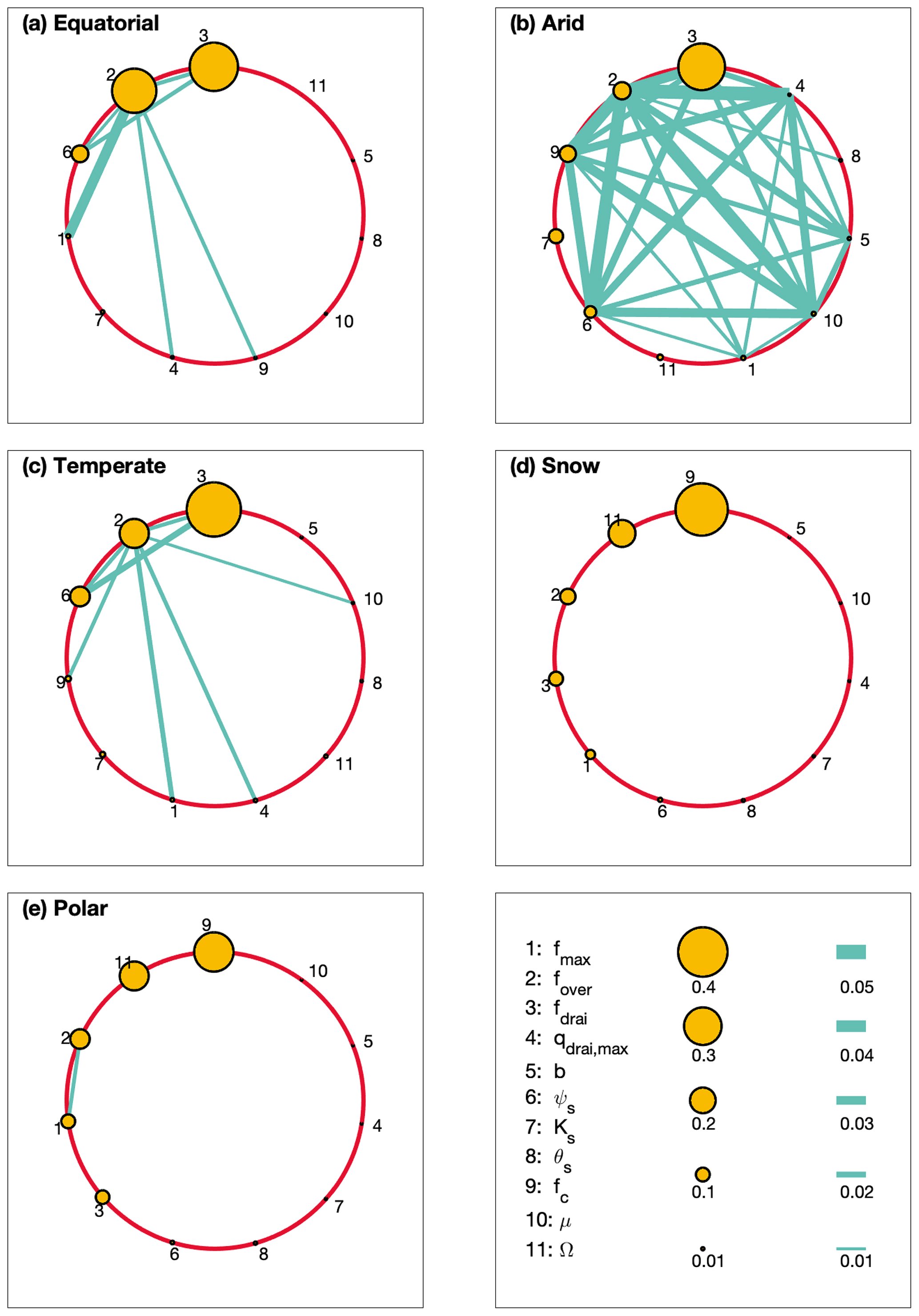
Figure 5Averaged main Sobol' index and joint Sobol' index for different climates defined by the Köppen climate classification. Only the cells with the relative norm 2 errors of PCE-based surrogate models for validating simulations of less than 0.15 are used for estimating the averaged sensitivity for each climate region. The size of the circles and thickness of the lines are proportional to main Sobol' index and joint Sobol' index, respectively. The legend in the right bottom subplot shows the Sobol' index for the corresponding size of circle and thickness of line.

Download

5.3 Global sensitivity analysis

The most significant ELM parameters identified for runoff generation are f_over, f_drai, ψ_s, f_c, and Ω, based on the spatial distribution of the main Sobol' indices (Fig. 4), while the other six parameters have negligible contributions to the runoff variations (Fig. S4). In equatorial regions, f_drai and f_over are equally sensitive and account for 39 % and 36 % of the average runoff variations, respectively, as indicated by the size of circles in Fig. 5a, while ψ_s is the secondary sensitive parameter. For the arid regions, f_drai is the most sensitive parameter, and f_over, f_c, K_s, and ψ_s are secondary sensitive parameters with a similar value for the main Sobol' indices (Fig. 5b). Although other parameters show negligible main Sobol' indices for arid regions, they have shown sensitivities when interacting with each other, as denoted by the thickness of the lines between each pair of parameters in Fig. 5b. The complex joint sensitivity results in high nonlinearity in the runoff variations, representing a possible reason for the poor performance of PCE for arid regions. The most significant uncertain parameters for the warm temperate region are the same as those for the equatorial region (Fig. 5c). Snow and polar climates have similar sensitivity pattern, with f_c and Ω being the two most important uncertain parameters (Fig. 5d and e). In colder regions, the contribution of surface water storage drainage, which is controlled by f_c, is large to the total runoff because of prominent surface water areas (Pekel et al., 2016). The hydraulic conductivity and groundwater drainage when ice is present in the soil is controlled by Ω, which has a significant impact on runoff-generation process when the soil is partial or fully frozen. The surface water storage and ice impedance factor, which were not included in the version of the model used in previous study (Hou et al., 2012; Huang et al., 2013), are found to be the most sensitive parameters in cold regions. Besides the arid region, other regions show smaller sensitivities to parameter interactions.

5.4 Parameter dimensionality reduction

The ELM simulated runoff is significantly sensitive to three or fewer parameters with Sobol' index >0.05 for 81.3 % of the total grid cells (Fig. S5). Therefore, we sampled only the three most sensitive parameters in each grid cell in the Markov chain Monte Carlo (MCMC) process to perform parameter inference, as mentioned in Sect. 3.3. The posteriors of the three calibrated parameters (f_drai, f_over, ψ_s) at an example grid cell (56.75^∘ W, 11.25^∘ S) are much more constrained than the priors after the MCMC simulation with the surrogate model (Fig. 6a, b, and c). The third parameter, ψ_s, has a relatively wider posterior than the first two parameters because its sensitivity is much smaller (e.g., Sobol' index = 0.08). The Gelman–Rubin R statistic of Gelman and Rubin (1992) computed with five MCMC chains (after the burn-in period) is 1.002, 1.004, and 1.003 for f_drai, f_over, and ψ_s, respectively, suggesting that our MCMC simulation has converged (see the convergence curve in Fig. S6). ELM simulations with a large number of samples from parameter priors are needed to identify the optimal parameter that minimizes RMSE; for example, 10 000 surrogate simulations are used to find the parameters that yield RMSE=1 (Fig. 6d). In contrast, due to the reduced parameter dimensionality and narrowed range, much fewer samples (e.g., 100) are needed to find the better parameter values (e.g., corresponding to RMSE<1) when they are sampled from the parameter posteriors (Fig. 6d). The spatial distribution of the parameter values at 5 % and 95 % of the posteriors is shown in Figs. S7 and S8, respectively.

Figure 6Posteriors of (a) f_drai, (b) f_over, and (c) ψ_s from parameter inference process at an example grid cell. Panel (d) shows the probability density function (PDF) of RMSE evaluated with surrogate models forced by 100 samples from parameter posteriors and 10 000 samples from parameter priors.

Download

5.5 Optimal parameter values

The procedure described in Sect. 3.5 is used to find the optimal parameter values for the three most sensitive parameters for each grid cell. For the grid cells with RE > 0.15 for surrogate models, the optimal parameter value is determined from the training and validation simulations (e.g., 200 simulations with random parameter values from priors) that yield minimum RMSE. The optimal parameter values show clear regional patterns (Fig. 7). Specifically, the optimal f_over tends to be lower than the default value for the equatorial and partial snow areas (Fig. 7a). The optimal f_over is found to be higher than the default value for the arid areas, while it is around the default value on average for the warm temperate areas (Fig. 7a). For the same water table depth, lower f_over leads to higher saturation fraction (Eq. 3), that in turn leads to larger surface runoff (Eq. 2). The calibrated f_drai is lower than the default value for both equatorial and arid regions (Fig. 7b). The optimal f_drai for warm temperate areas show different patterns, with higher values over eastern USA and Europe but lower values over southeastern China. The generation of subsurface runoff depends on f_drai (Eq. 8), with lower f_drai leading to larger subsurface runoff. ψ_s affects the runoff generation through its impact on soil water movement, such as the soil water flux being larger at saturation with higher ψ_s. As shown in Fig. 7c, higher ψ_s are needed to minimize the RMSE for all regions that show sensitivity to this parameter, except for some grid cells from polar area. Over the high latitudes of Northern Hemisphere, higher f_c and lower Ω are found in the optimal parameters (Fig. 7d, e). The surface water storage can store more water at higher f_c by reducing surface water runoff (Eqs. 4, 7), thus leading to a lower and delay peak runoff than the default values. Furthermore, the lower Ω values have fewer impacts of ice on hydraulic conductivity (Eq. 7.89 in Olson et al., 2016) and drainage (Eq. 9), leading to higher runoff for the winter seasons.

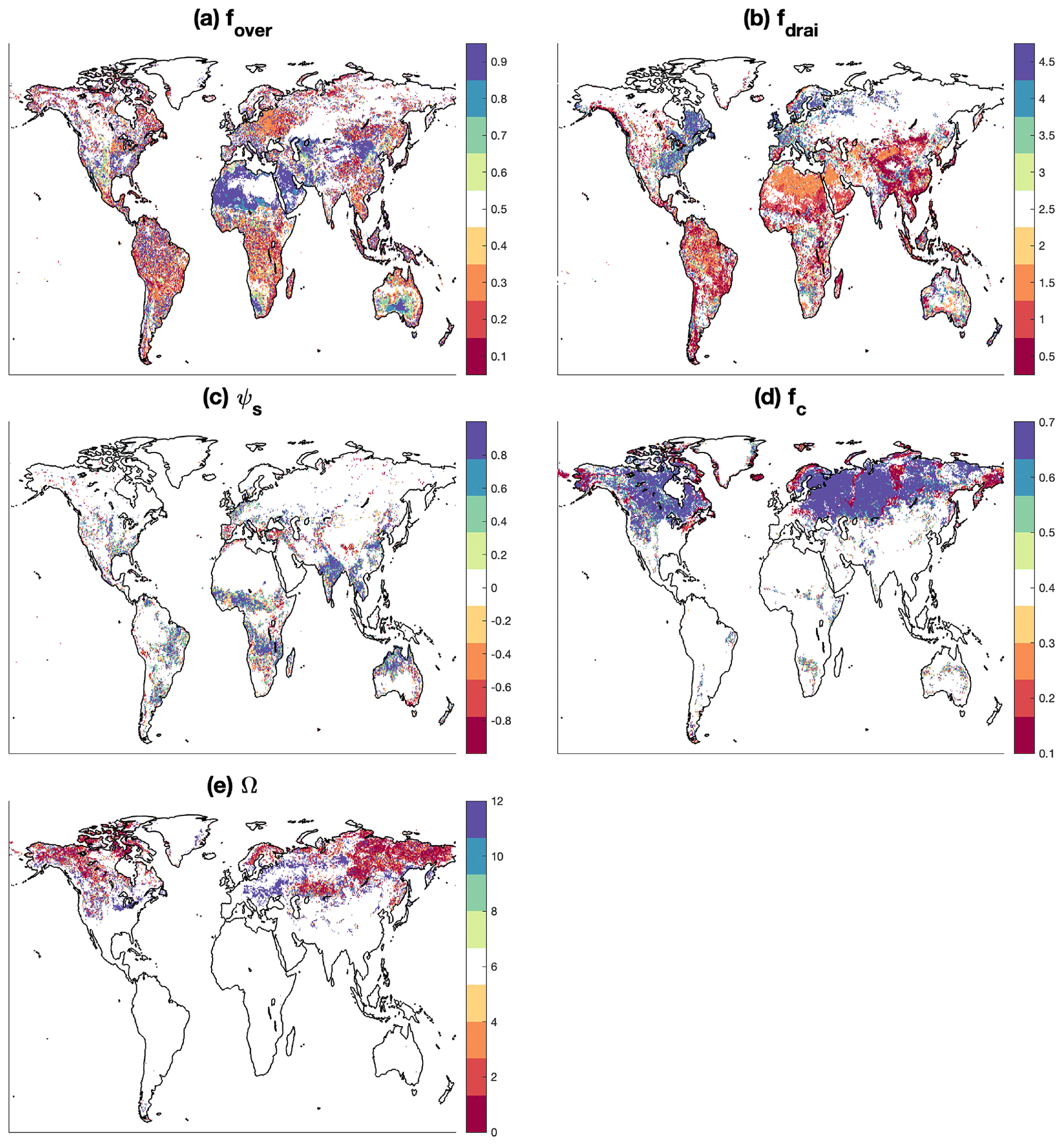
Figure 7Optimal values for the sensitive parameters. The default values for the parameters are defined at the midpoint of the color map. There are no certainty bounds for ψ_s from different grid cells because it is determined by the soil properties. Therefore, the values of ψ_s are scaled to [−1, 1] in panel (c) for each grid cell with the corresponding upper bound (ψ_s,max) and lower bound (ψ_s,min): $\frac{\mathrm{2}}{{\mathit{\psi }}_{\mathrm{s},\max }-{\mathit{\psi }}_{\mathrm{s},\min }}{\mathit{\psi }}_{\mathrm{s}}-\frac{{\mathit{\psi }}_{\mathrm{s},\max }+{\mathit{\psi }}_{\mathrm{s},\min }}{{\mathit{\psi }}_{\mathrm{s},\max }-{\mathit{\psi }}_{\mathrm{s},\min }}$.

5.6 Evaluation of ELM with the optimal parameters

The ELM-simulated runoff with the optimal parameter values shows improved skills of capturing the spatiotemporal variation in monthly runoff at a global scale with higher NSE and KGE compared to the simulation with default parameter values (Fig. 8). Specifically, the median of NSE and KGE from all global grid cells increases from −0.88 and −0.05 to 0.06 and 0.31, respectively. Over the western USA coast, southeast and midwest of USA, western Europe, and equatorial areas, the performance of the calibrated ELM is better with NSE > 0.5 and KGE > 0.7. While the performance of other areas (e.g., western USA, Sahara and Arabian desert, central and eastern Asia, and partial high latitude regions) is improved compared to simulations with the default parameter values, the NSE and KGE still have negative values. The higher model errors in those regions cannot be resolved by calibration as (1) the simulation resolution is too coarse to resolve the topographic impacts (Chegwidden et al., 2020), (2) the snow-melting processes are not calibrated in this study, and the onset of snowmelt in ELM is poorly represented (Toure et al., 2018), and (3) the hydrology of arid areas is not well understood (Pilgrim et al., 1988). Except for the calibration period, ELM with the optimal parameters also shows an improved performance in runoff simulation for another period (2011–2013; Fig. S9).

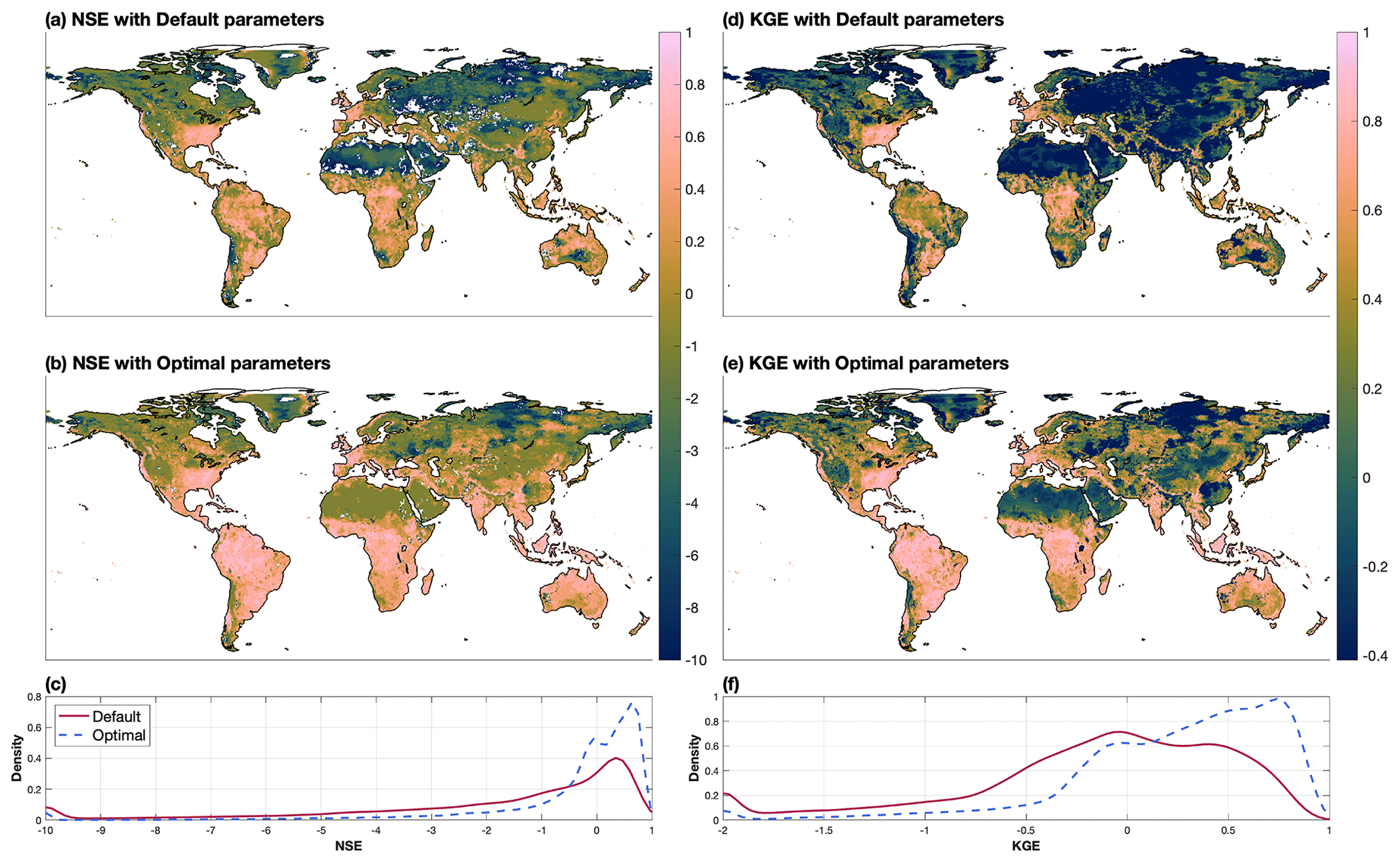
Figure 8Evaluation of simulated monthly runoff for 1991–2010 at grid level with default and optimal parameters. Panels (a) and (b) show the NSE metrics between the GRUN runoff and simulated runoff with default and optimal parameters, respectively. Panel (c) shows the comparison of the probability density function (PDF) of NSE metrics from all the global grid cells. Panels (d), (e), and (f) illustrate the evolution with the KGE metric.

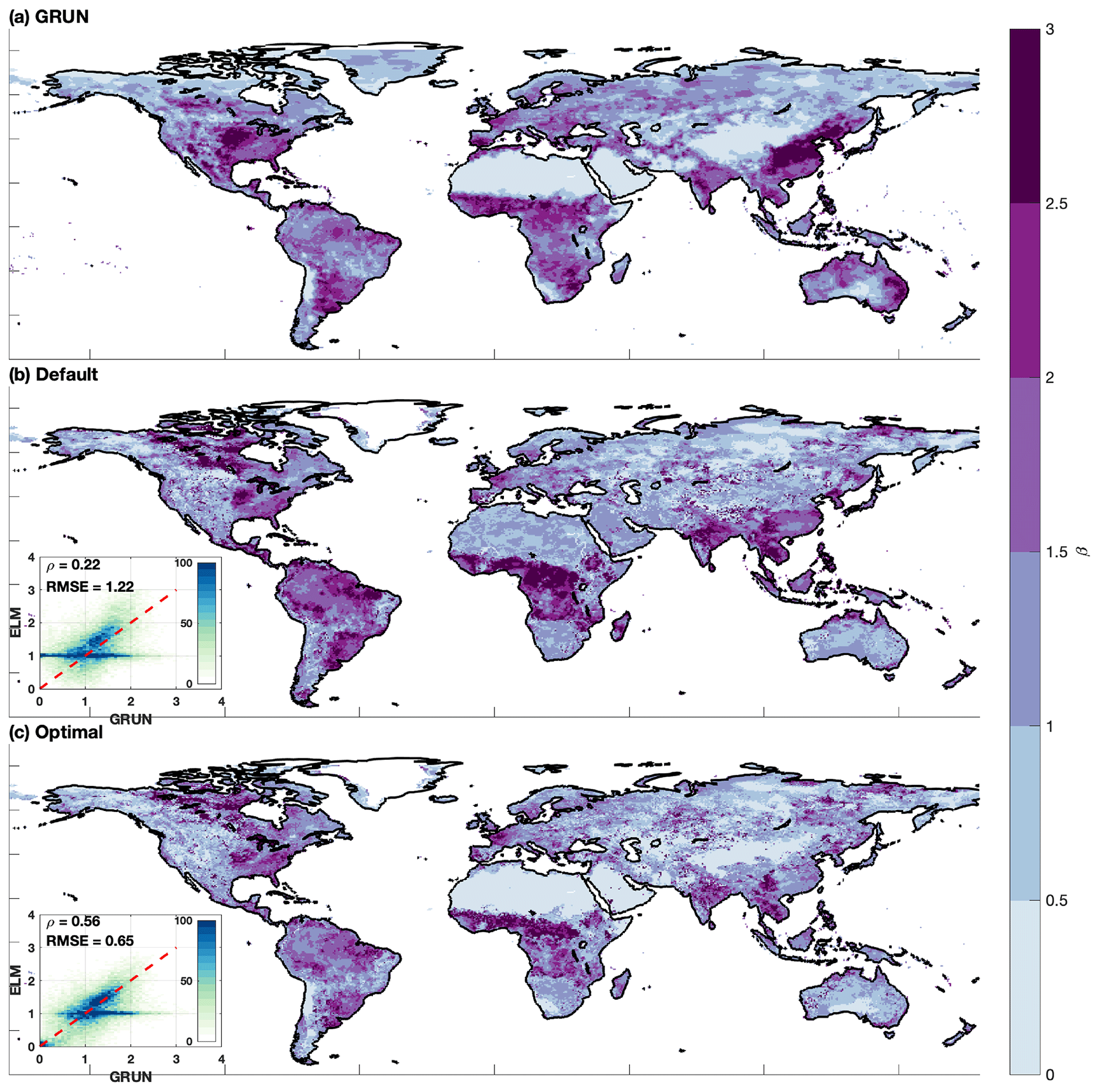
Figure 9Sensitivity of runoff to precipitation (β) estimated from the (a) GRUN runoff dataset, (b) ELM simulation with default parameter, and (c) ELM simulation with optimal parameter. The inserts show the scatterplots with density for cell-to-cell comparison of β between GRUN and ELM simulations.

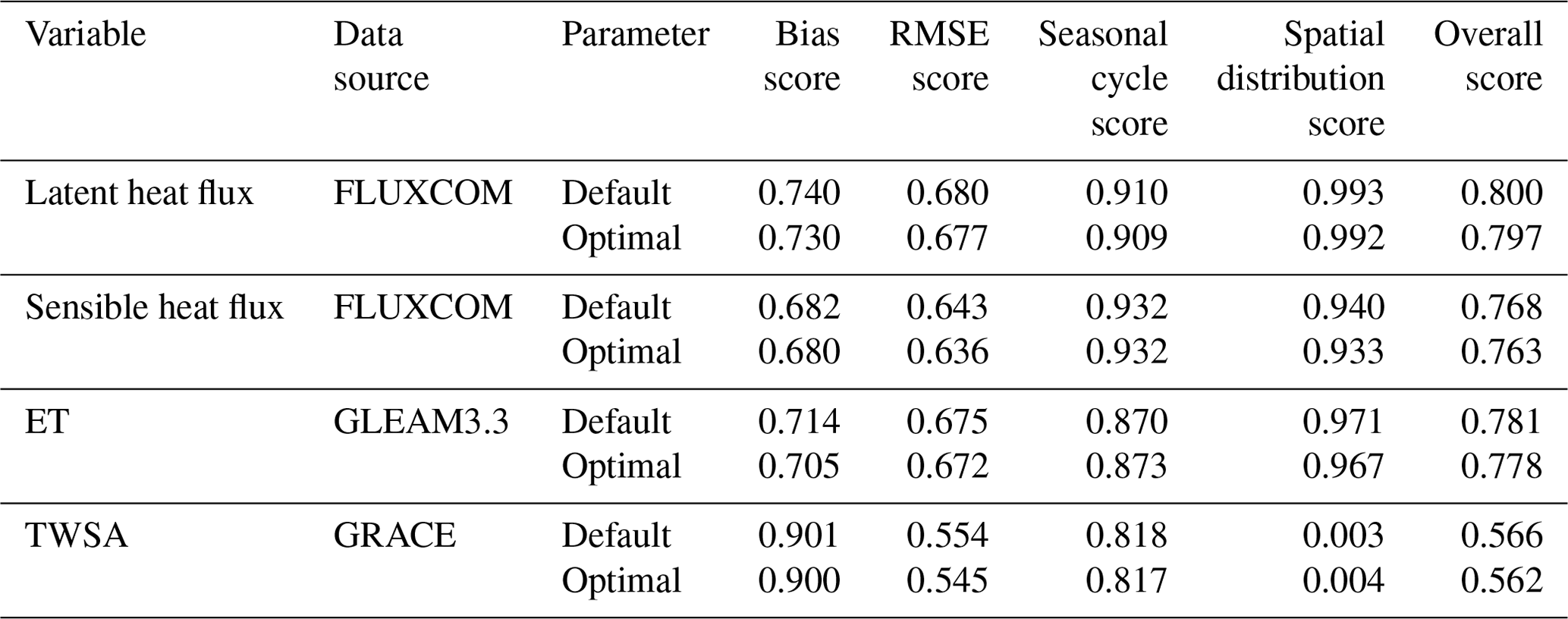
Table 2ILAMB benchmark scores for latent heat flux, sensible heat flux, evapotranspiration, and terrestrial water storage anomaly with default and optimized parameters in ELM. A description of each score metric can be found at http://redwood.ess.uci.edu/CMIP6_bnchmrk1_9_8/ (last access: 23 June 2021).

Download Print Version | Download XLSX

Compared to the reference runoff (Fig. 9a), the ELM simulation with default parameter values tends to overestimate the sensitivity of runoff to precipitation (β in Eq. 24) for the equatorial and arid regions but underestimates β in the warm temperate regions, such as the eastern USA, China, and eastern coast of Australia (Fig. 9b). The simulation with optimal parameter values is able to more accurately estimate β than the simulation with default parameter values with improved spatial correlation coefficient from 0.22 to 0.56 and lower RMSE from 1.22 to 0.65 (Fig. 9c). However, some significant discrepancy of β still exists in the simulation with optimal parameter values (e.g., eastern China), implying that the sensitivity is not well constrained in ELM for certain regions even after model calibration.

According to the evaluation with the ILAMB package, ELM shows a similar performance in simulating other variables (e.g., latent heat flux, sensible heat flux, ET, and TWSA) with optimal parameter values compared to the use of the default parameter values (Table 2). However, both the default and optimal simulations fail to capture the spatial variation in TWSA with a spatial distribution score of less than 0.05. This is because the coarse resolution (e.g., several hundred kilometers) of GRACE product (Seyoum et al., 2019) cannot resolve the spatial variability in TWSA for our model resolution.

5.7 Parametric uncertainty

The parameter priors listed in Table 1 result in significant uncertainties in the total runoff, with the global average annual runoff for 1991–2010 varying from 30 999–76 496 km³ yr⁻¹ (Fig. 10a). After parameter inference, the uncertainty of the runoff constructed using simulations with parameter posteriors is constrained to 35 389–49 741 km³ yr⁻¹. The constrained annual runoff uncertainty captures the reference runoff (38 443 km³ yr⁻¹) and is consistent with previous global runoff studies (Schellekens et al., 2017; Rodell et al., 2015; Clark et al., 2015; Haddeland et al., 2011). The simulation with the optimal parameter values yields an averaged global annual runoff of 42 156 km³ yr⁻¹, overestimating the reference runoff by 9.6 %. The overestimation is mainly from the Amazon, Asia, and eastern Europe (Fig. 10b), and Ghiggi et al. (2019a) reported a similar spatial bias pattern between global hydrological model simulations in ISIMP2a. The simulation with the default parameter values shows smaller biases in terms of the annual runoff magnitude as compared to the reference runoff data, with an overestimation of 5.3 % on average. However, the smaller biases of annual runoff with the default parameters are because of the canceling out of the monthly errors to some extent. For example, the default parameters tend to overestimate the runoff during the wet periods but underestimate the runoff during the dry periods in the Amazon basin (Fig. S10a). While the default simulation shows higher RMSE and lower NSE at a monthly scale, it yields smaller biases at an annual scale than the optimal parameter (Fig. S10b). Therefore, the calibrated simulation shows better performance in capturing the spatiotemporal variability (higher NSE and KGE in Fig. 8b and e), but it does not lead to a reduced bias at an annual scale. We further acknowledge that 200 simulations with 11 random parameters may not be sufficient to capture the full variations in simulated runoff.

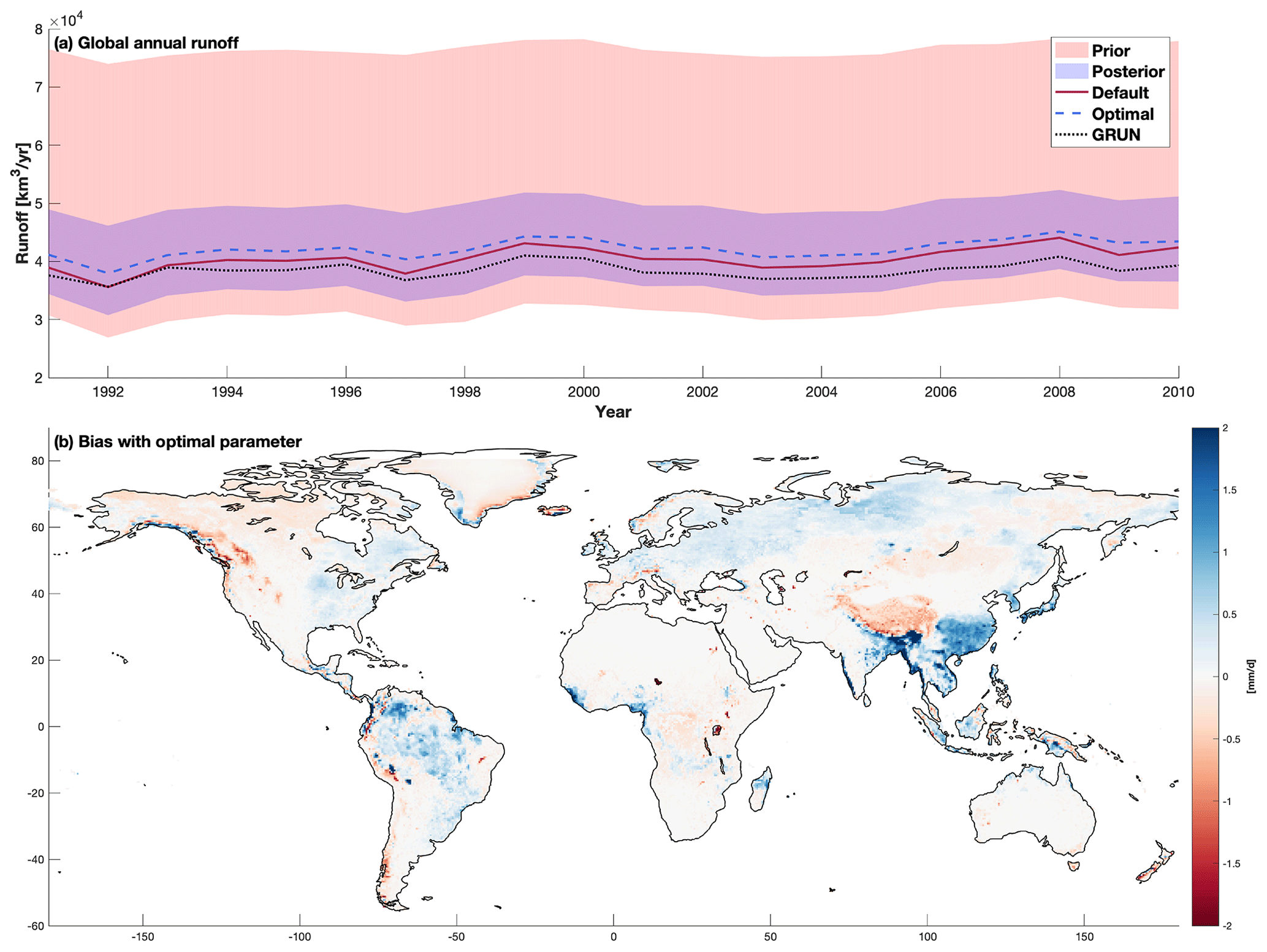
Figure 10(a) Annual global runoff from default ELM simulation, optimal ELM simulation, and GRUN runoff dataset for the simulation period (1991–2010). The red and blue shade areas represent the uncertainties constructed from the simulations with the parameter sampled on priors and posteriors, respectively. Panel (b) shows the absolute difference in annual average runoff between ELM simulation with optimal parameter and GRUN runoff data.

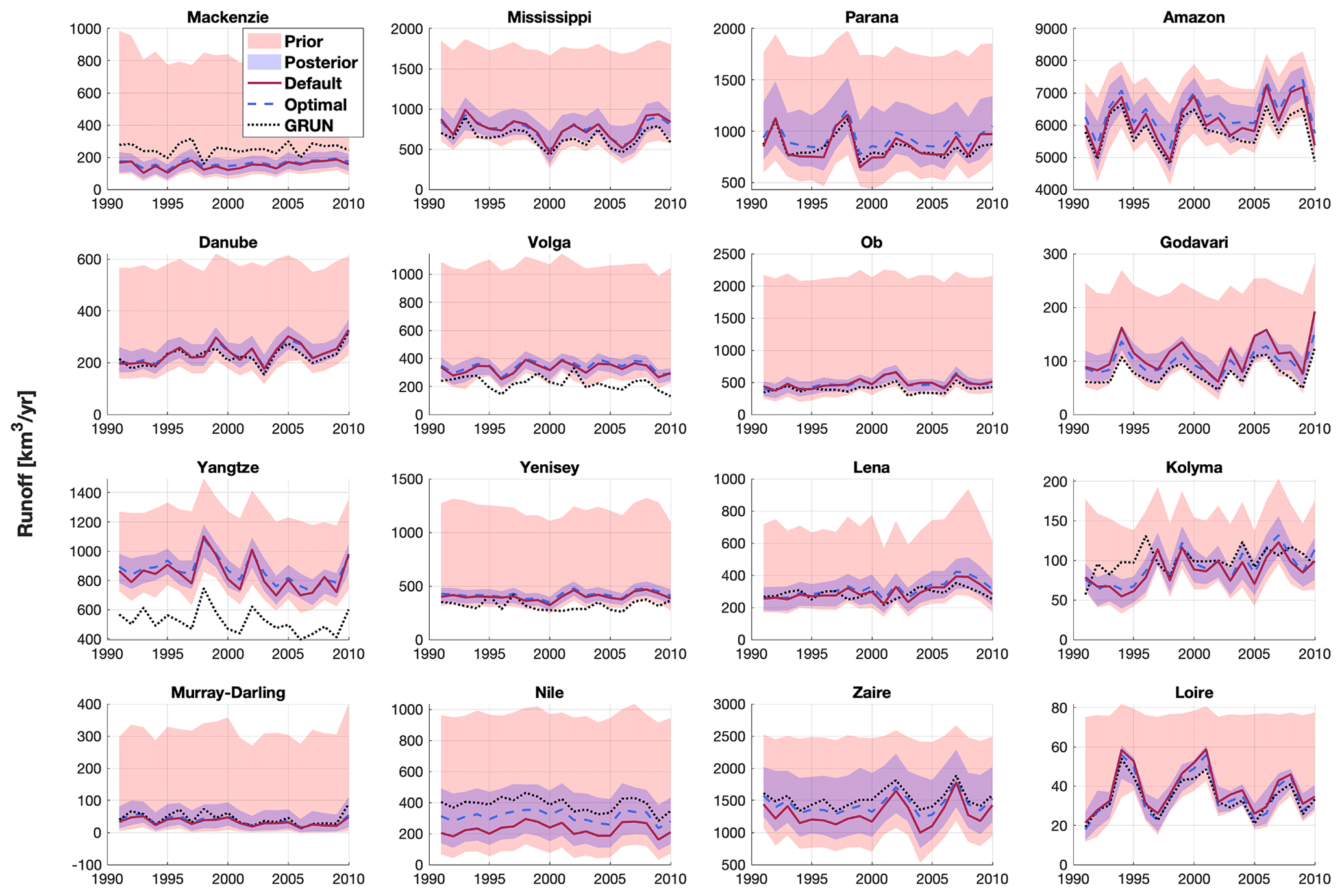
Figure 11Annual runoff at basin scale from the default ELM simulation, optimal ELM simulation, and GRUN runoff dataset for the simulation period (1991–2010). The red and blue shaded areas represent the uncertainties constructed from the simulations with parameter sampled on priors and posteriors, respectively.

Download

Figure 12(a) Annual global runoff from 13 global hydrological models participated in ISIMIP2a and ELM simulated runoff uncertainty constructed using simulations with parameter posteriors. (b) Sen's slope for the global annual runoff for the GRUN runoff dataset and simulations. The violin plots (Hintze and Nelson, 1998) are generated with Sen's slope of ELM simulations with parameter posteriors. The white point is the median value, and the gray line represents range of the 25 %–75 % percentile. The MATLAB function of Bechtold (2016) was used to create the violin plot. The cross signs are the Sen's slopes estimated from the ISIMIP2a model simulations.

Download

The runoff uncertainties associated with parameters are constrained significantly with the parameter posteriors at basin scale as well (Fig. 11). Noticeably, the posterior uncertainty of annual runoff is larger over the equatorial regions (e.g., Paraná, the Amazon, Godavari River, and Congo River) than other regions. The simulation with optimal parameter values yields larger overestimation of total runoff compared to the simulation using the default parameter values for the selected basins, except for the Mississippi River, Godavari River, and Loire basin (Table S1 in the Supplement). The reason for the overestimations is that the optimal parameters are determined by maximizing NSE at a monthly scale, which cannot ensure that the annual runoff is appropriately constrained. There exist significant discrepancies between simulations and GRUN for basins located at high latitudes (e.g., Mackenzie, Volga, Ob, Yenisei, and Lena rivers) even when the posterior uncertainties are considered (Fig. 11), highlighting the importance of snow-melting processes in snow-dominated regions. However, the large difference between ELM and the reference runoff in Yangtze River basin may be caused by the bias of the reference runoff since a previous study reported annual discharge to be around 900 km³ yr⁻¹ (Yang et al., 2015).

Despite being constrained by the parameter inference process, the parametric uncertainty of ELM-simulated annual runoff is considerable. Specifically, the posterior uncertainty of global runoff simulated by ELM is comparable to that of the multimodel ensemble constructed with the 13 global hydrological models from ISIMIP2a (Fig. 12a). The parametric uncertainty affects not only the magnitude of global runoff but also the trend for the simulation period during which a rapid increase in temperature has occurred (Fig. S11a). The Sen's slope (Sen, 1968) for the reference runoff data is found to be 54.7 km³ yr⁻¹, but this increasing trend is not significant according to the Mann–Kendall test (Fig. 12b). Other studies also reported no significant changes in the global runoff with observed streamflow data (Alkama et al., 2013; Dai et al., 2009; Milliman et al., 2008; Alkama et al., 2011). However, the default and calibrated ELM simulations yielded the Sen's slope to be 188.9 and 133.8 km³ yr⁻¹, respectively. Although the Sen's slope is reduced with the optimal parameters, the increasing trend remains significant. Likewise, all the other global hydrological models of ISIMIP2a exhibit significant increasing trend in the annual runoff, with the Sen's slope varying from 93 to 272 km³ yr⁻¹ (Fig. 12b). Considering that the GRUN dataset and all model simulations are forced by the same atmosphere forcing (i.e., GSWP3), the differences in the global runoff trends can be attributed to the model structural/parametric uncertainty. We note that there exists a significant trend in GSWP3 precipitation at a global scale, with an increase of 246.1 km³ yr⁻¹ during the simulation period (Fig. S11b). But it remains unclear how the runoff responds to the increase in precipitation at a global scale because the concurrent increased temperature (Fig. S11a) leads to more ET, which can potentially balance the increased precipitation to some extent. The inconsistency of the global runoff trend between the model simulations and observation-based data can be caused by uncertainties of different sources. For example, the accuracy of GRUN is limited by the coverage of the streamflow gauges, as over half of the global areas are ungauged (Alkama et al., 2013). The model parametric uncertainty is significant, as ELM simulations with parameters posteriors show a wide range of annual runoff trend, from no trend to a significant increasing trend (Fig. 12b). This highlights the necessity of including parametric uncertainty in future runoff projections, since runoff trend is not well constrained even if the model performance in the control period is improved.