the Creative Commons Attribution 4.0 License.
the Creative Commons Attribution 4.0 License.
 | 29 Mar 2018
Increase in flood risk resulting from climate change in a developed urban watershed – the role of storm temporal patterns
Suresh Hettiarachchi
Conrad Wasko
The effects of climate change are causing more frequent extreme rainfall events and an increased risk of flooding in developed areas. Quantifying this increased risk is of critical importance for the protection of life and property as well as for infrastructure planning and design. The updated National Oceanic and Atmospheric Administration (NOAA) Atlas 14 intensity–duration–frequency (IDF) relationships and temporal patterns are widely used in hydrologic and hydraulic modeling for design and planning in the United States. Current literature shows that rising temperatures as a result of climate change will result in an intensification of rainfall. These impacts are not explicitly included in the NOAA temporal patterns, which can have consequences on the design and planning of adaptation and flood mitigation measures. In addition there is a lack of detailed hydraulic modeling when assessing climate change impacts on flooding. The study presented in this paper uses a comprehensive hydrologic and hydraulic model of a fully developed urban/suburban catchment to explore two primary questions related to climate change impacts on flood risk. (1) How do climate change effects on storm temporal patterns and rainfall volumes impact flooding in a developed complex watershed? (2) Is the storm temporal pattern as critical as the total volume of rainfall when evaluating urban flood risk? We use the NOAA Atlas 14 temporal patterns, along with the expected increase in temperature for the RCP8.5 scenario for 2081–2100, to project temporal patterns and rainfall volumes to reflect future climatic change. The model results show that different rainfall patterns cause variability in flood depths during a storm event. The changes in the projected temporal patterns alone increase the risk of flood magnitude up to 35 %, with the cumulative impacts of temperature rise on temporal patterns and the storm volume increasing flood risk from 10 to 170 %. The results also show that regional storage facilities are sensitive to rainfall patterns that are loaded in the latter part of the storm duration, while extremely intense short-duration storms will cause flooding at all locations. This study shows that changes in temporal patterns will have a significant impact on urban/suburban flooding and need to be carefully considered and adjusted to account for climate change when used for the design and planning of future storm water systems.
- Article
(5753 KB) -
Supplement
(585 KB) - BibTeX
- EndNote


Recent history shows that extreme weather events are occurring more frequently and in areas that have not had such events in the past (Hartmann et al., 2013). There are more land regions where the number of heavy rainfall events has increased compared to where they have decreased (Alexander et al., 2006; Donat et al., 2013; Westra et al., 2013a). Intensification of rainfall extremes (Lenderink and van Meijgaard, 2008; Wasko and Sharma, 2015; Wasko et al., 2016b) and their increasing volume (Mishra et al., 2012; Trenberth, 2011) has been linked to the higher temperatures expected with climate change. This increase in the likelihood of extreme rainfall and its intensification creates a higher risk of damaging flood events that cause a threat to both life and the built environment, particularly in urban regions where the existing infrastructure has not been designed to cope with these increases. Adapting to future extreme storm events (i.e., flood events) will be costly both economically and socially (Doocy et al., 2013). Properly addressing this increased flood risk is all the more important given the expectation that the urban population is projected to grow from the current 54 to 66 % of the global population by the year 2050 (United Nations, 2014).
Adaptation as a way to address the effects of climate change has only recently attracted attention (Mamo, 2015; Füssel, 2007). Adaptation in the context of flood risk involves taking practical and proactive action to adjust or modify (Adger et al., 2007) storm water management infrastructure such as low impact development (LID) methods to reduce surface runoff or constructed storage to handle the increased flows during an extreme storm. The foundation of adaptation measures to deal with flooding is typically based on flood forecasting and hydrologic and hydraulic (H–H) modeling (Thodsen, 2007). The effectiveness of adaptation is dependent on the accuracy of simulating projected impacts, such as the effectiveness of a flood control structure to protect a city from future increased flooding. In addition, variability and uncertainty related to these flood forecasts play an important role since uncertainty in future projection limits the amount of adaptation that society will accept (Adger et al., 2009). Prior to the advent of computers and the increase in computational power, drainage design was based on simple empirical models of peak discharge rates using methods such as the rational formula in combination with intensity–duration–frequency (IDF) curves (Adams and Howard, 1986; Nguyen et al., 2010; Packman and Kidd, 1980). Consideration of the environmental impacts related to flow rates, volumes, water quality and downstream impacts requires more complex systems and ways to simulate the hydrologic and hydraulic processes in a more realistic manner (Nguyen et al., 2010). As such, the state of the art in modeling urban sewer and storm-water-related infrastructure uses distributed, fully dynamic, hydrologic and hydraulic modeling software (Singh and Woolhiser, 2002). The dynamic approach and integrated nature of current modeling requires the use of temporal patterns to distribute rainfall and volumes that closely resemble actual storm events (Nguyen et al., 2010; Rivard, 1996).
Temporal patterns have typically been derived using the alternating block method from IDF curves, where shorter storm durations are nested within longer storm duration design intensities (García-Bartual and Andrés-Doménech, 2017; Mockus et al., 2015). However, this method does not represent a real storm structure. Alternatively, Huff (1967) presented the first rigorous analysis of rainfall temporal patterns (García-Bartual and Andrés-Doménech, 2017), where rainfall temporal patterns were derived from observations. Similar methods include the average variability method, where a storm is partitioned into fractions of equal time, and each fraction is ranked. The temporal distribution is then specified as the most likely rainfall order with the average rainfall used for the associated fraction (Pilgrim et al., 1997). The National Oceanic and Atmospheric Administration (NOAA) Atlas 14 provides an updated set of temporal distributions and IDF curves for use in a major portion of the United States (Perica et al., 2013) that are now widely used for planning and design modeling analysis. These temporal distributions and rainfall depths are based on observed data and were generated using methodology similar to Huff (1967). The major concern is that the analysis and methods used in Atlas 14 assume a stationary climate over the period of observation and application (chap. 4.5.4 of Atlas 14 Volume 8). This seems contrary to prevailing scientific thought (Milly et al., 2007) and can lead to inadequacies of future storm water infrastructure as there is evidence to believe that warmer temperatures are forcing the intensification of temporal patterns (Wasko and Sharma, 2015) and an increase in variability (Mamo, 2015). Several previous studies have examined the sensitivity of urban catchments to changes in intensity and temporal patterns, by modeling peak runoff rates and volumes (Lambourne and Stephenson, 1987; Mamo, 2015; Nguyen et al., 2010; Zhou et al., 2017). For example, Lambourne and Stephenson (1987) presented a comparative model study to look at the impact of temporal patterns on peak discharge rates and volumes. However, with the exception of Zhou et al. (2018), these studies largely ignored the detailed hydraulic conveyance aspects of storage ponds, sewers, culverts and flow control structures which play an important role in how the flow rates generated during runoff move through and impact the built environment.
Although there are an increasing number of catchment/basin-scale and urban modeling studies that have been performed (Cameron, 2006; Graham et al., 2007; Leander et al., 2008; Zhou et al., 2018; Zope et al., 2016), there is a lack of a detailed studies that look at assessing future flood damage in a developed environment (Seneviratne et al., 2012). The majority of past studies focus on either the hydrologic modeling component or the rainfall intensity aspect and mostly overlook the crucial detail of rainfall patterns. In this study, we focus on the range of results generated from detailed H–H modeling arising from precipitation pattern variability and the impact of climatic change. We pay particular attention to the assessment and illustration of the variability in how different catchments respond to different rainfall patterns and the impacts of climate change. The primary questions that we address are as follows.
-
What is the relative importance of the storm pattern and volume of rainfall on urban flood peaks?
-
How will climate change affect storm patterns and volumes and what are the impacts on urban flood peaks?
Flood risk assessment and communication depend on flood risk mapping, for which flood inundation areas are needed (Merz et al., 2010). Urban catchments are typically complex and need to capture the response of the system along with the interactions of the various components of the storm water infrastructure (Zoppou, 2001) to provide reliable flood depths to develop inundation areas. The main characteristic of storm water in urban areas is that the flows are predominantly conveyed in constructed systems, replacing or modifying the natural flow paths. Including the complex hydraulics and possible hydraulic attenuation and timing of congruent flows will have an impact on flooding, particularly in developed environments. As discussed, temporal patterns of rainfall are now a critical aspect of the design and planning of future storm systems. Research which uses temperature to project future rainfall and temporal patterns and then assesses impacts on flooding has not yet been performed. This study aims to fill this research gap through an elaborate analysis of how rainfall intensities and patterns impact urban flood risk in a warmer climate.
Developed urban areas present the highest probability of causing damage and loss of life during flood events. There has been an increase in urban flooding in the past decade, with densely populated developing countries like India and China coming into focus (Bisht et al., 2016; Zhou et al., 2017; Willems et al., 2012). A case study on the Oshiwara River in Mumbai, India, has shown a 22 % increase in the overall flood hazard area due to changes in land use and increased urbanization within the catchment (Zope et al., 2016). In particular, flooding in Mumbai in 2005, which was caused by extreme rainfall coupled with inadequate storm sewer design, is blamed for 400 deaths (Bisht et al., 2016). China also experienced a devastating flood season in 2016 (Zhou et al., 2018) with the rapid increase in urbanization. Even with better planned and mature urban cities, Europe and North America are not immune to flooding in urban areas (Ashley et al., 2005; Feyen et al., 2009; Smith et al., 2016; Sandink, 2015). Impacts of climate change are expected to increase the risk of flooding and further exacerbate the difficulty of flood management in developed environments.
The number of studies investigating climate change impacts on urban flooding is increasing as the importance of this topic is more and more recognized. However, research focusing on the impacts of climate change on precipitation temporal patterns remains limited. The majority of available research uses global circulation models (GCMs) and regional climate models (RCMs) combined with statistical downscaling techniques to project IDF curves to reflect future climate conditions (Mamo, 2015; Nguyen et al., 2010; Schreider et al., 2000; Raff et al., 2009; Sørup et al., 2016). For example Mamo (2015) used monthly mean wet weather scenario data projected by four GCMs for the period 2020–2055, along with historic data from 1985 to 2013, which were then used as weather generator input using LARS-WG, from which data were generated to develop revised IDF curves. Nguyen et al. (2010) used data sets generated by two separate GCMs to develop IDF and temporal patterns to reflect future rainfall patterns. The inconsistent results generated by the two different GCMs illustrate the challenge of forecasting future climate conditions using GCM-generated results. It is recognized that GCM results form the largest part of the uncertainty in projected flood scenarios (Prudhomme and Davies, 2009).
Alternatively, research has shown that temperature, which influences the amount of water contained in the atmosphere, can have an impact on the patterns and total rainfall volumes of storm events (Hardwick Jones et al., 2010; Lenderink and van Meijgaard, 2008; Molnar et al., 2015; Utsumi et al., 2011; Wasko et al., 2015; Westra et al., 2013a). In general, intensification of rainfall events is expected with a trend towards “invigorating storm dynamics” (Trenberth, 2011; Wasko and Sharma, 2015). Even though forecasts for climate change impacts on future flooding have a “low confidence”, global-scale trends in temperature extremes are more reliable (Seneviratne et al., 2012). Following successful studies (Wasko and Sharma, 2017; Westra et al., 2013b) we take the approach of using temperature to project temporal patterns and rainfall volume to account for climate change impacts. As described in detail in Sect. 5, we examine historical rainfall data coupled with daily average temperature to project temporal patterns and rainfall volumes to account for climate change impacts.
In this study we use temperature to project rainfall temporal patterns and volumes to evaluate the variability in flood risk as well as the impact on flood risk due to climatic change. Broadly, the steps taken are as follows:
-
application of multiple temporal patterns and rainfall volumes with their associated confidence limits in the H–H model to establish the variability in the flood risk;
-
development of scaling factors (Lenderink and Attema, 2015; Wasko and Sharma, 2015) for the volume and temporal pattern for future conditions using temperature as the index;
-
evaluation of the impact of temperature rise on flood risk by scaling temporal patterns for a temperature increase;
-
evaluation of the cumulative impact of temperature rise on flood risk by scaling both volume and temporal patterns.
The hydrologic and hydraulic modeling performed here used the EPA SWMM model of an urban/suburban catchment in Minneapolis, Minnesota, United States. The SWMM software package was initially developed by the US Environmental Protection Agency (EPA, 2016) and has since been used as the base engine for most of the industry standard H–H modeling packages.
4.1 Study location and model
The H–H model used in this study was developed for the South Washington Watershed District (SWWD) in the state of Minnesota, United States, for the management of surface water flows as well as for the planning and management of ongoing development work and capital improvement projects. The catchment area of the SWWD is a highly developed urban/suburban area and extends over 140 km2. The model was initially built in the year 2000 and has been continuously maintained and updated with the latest available land use/land cover and storm water infrastructure information. The model includes extensive detail of all land use types and storm water infrastructures including sewers, culvert crossing, open-channel reaches, and constructed as well as natural storage. Highly detailed delineation of both sub-catchment boundaries and impervious area was done using a high-resolution digital elevation model, development construction and grading plan overlays and aerial imagery within a GIS environment. All surface runoff is fed into the appropriate inflow points of the hydraulic conveyance system. The model has been validated and used to design major capital improvement and flood mitigation projects (Hettiarachchi et al., 2005). Additional model information is available in the Supplement Sect. S1. For the purposes of this study and to reduce the complexity and model run times, the model was trimmed to the upper section of the SWWD, representing an area of approximately 22 km2.

Figure 1Location of the model and the sub-watersheds along with the reference points used in the discussion below. The details of the reference points and further explanation are presented in Table 1. The orange lines are an example of the sewer network geometry in the model. The blue lines represent reaches that are open channel. The magenta lines are the surface overflow routes that capture flow that tends to flood in areas and spread outside the sewer network. The black lines provide connectivity when the georeferenced locations of nodes are geographically different to the ends of some of the sewer network.
Figure 1 presents the focus areas along with the schematic of the model network to illustrate the level of detail of the existing storm water infrastructure captured in the model. As discussed above, the model includes geometry details to explicitly model the street overflow routes where flooding occurs as well as depth/area curves that capture flooding at the storage nodes. This level of detail results in accurately modeling the travel time of flows within the watershed and capturing all the runoff volume generated from the storm. Additionally, the geometry details provide a reasonably accurate representation of extents related to flooding. The proper simulation of hydraulic attenuation and a variety of land use types provide an ideal platform for this study.
Table 1Description of reference locations presented in Fig. 1 and used to present results. Each location represents a variation of land use within the watershed.
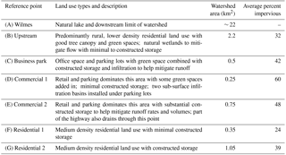
Table 1 lists the primary reference locations that are used for this study. The locations have specifically been chosen to represent the range of possible conditions that are encountered in urban catchments. The sub-catchment sizes vary from less than 0.5 km2 to approximately 2 km2, with an overall catchment of 22 km2. Different land uses such as commercial and industrial or different types of residential areas, as well as the amount of storage, have all been considered. It is important to note that these locations were selected prior to any model runs or availability of results and hence do not bias the results presented. Table 1 gives a description of the primary land use type of the subwatershed that drains to each reference location along with the watershed area and the overall percentage of impervious surface area within that watershed. It also describes whether there are local storage ponds, either natural or constructed, that provide rate and volume control.
4.2 Precipitation and temperature data
The precipitation and temperature data used in the analysis were sourced from the NOAA. Both hourly and daily rainfall data were downloaded from the climate data website for the Minneapolis–St Paul (MSP) International Airport gauge, which is the closest major airport to the study area. Daily data for the MSP airport were available from 1901 to 2014, while hourly data were available from 1948 to 2014. Daily maximum, minimum and average temperature data were also downloaded for the period from 1901 through 2014. For this analysis days that did not have precipitation data were assumed to have no rain.
Table 2Description of notation used in reference to the modeled storm depths and temporal distributions (NOAA Atlas 14 Volume 8 Appendix 5 accessed from http://www.nws.noaa.gov/oh/hdsc/PF_documents/Atlas14_Volume8.pdf) (see Fig. 2). ARI represents the average recurrence interval.
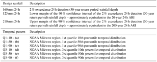
The temporal patterns for storms and the depths of rainfall were taken from NOAA ATLAS 14 Volume 8 (Perica et al., 2013) – the current state-of-the-art design standard for this location. The modeling analysis was centered on the 50-year (2 % exceedance probability) storm, which has a total rainfall volume of 160 mm in 24 h, for the area within the SWWD in the United States. The 90 % confidence margin storm depths were added to the analysis to look at how modeled flood depths vary with total precipitation (Table 2). Six temporal distributions (two patterns with their associated confidence margins) were chosen from NOAA ATLAS 14 Volume 8 to investigate how flood depths are impacted by the shape of storm over a 24 h period. Table 2 describes the different storm temporal patterns and each of the precipitation volumes modeled. The spatial distribution of rainfall is assumed to be uniform for this study. Even though we acknowledge that spatial variability of rainfall can have an impact on flooding, adding that dimension to the current analysis would have made the level of effort excessive. Also, by not spatially varying the rainfall distribution, we are able to better focus on the sensitivity of temporal patterns on flooding impacts.
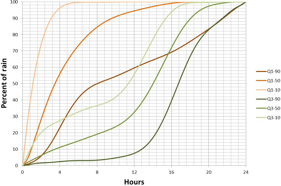
The quartiles indicate the timing of the greatest percentage of total rainfall that occurs during a storm. The first quartile indicates that the majority of the rainfall, including the peak, occurs in the first quarter of the duration, which is between hours 1 and 6 in the case of a 24 h storm. The third quartile indicates that the majority of the rainfall, including the peak, occurs in the third quarter of the storm duration, that is, hours 12–18 in the case of a 24 h storm. The temporal distributions were also separated in Atlas 14 to determine the frequency of occurrence within each quartile to determine a percentile for each distribution.
The SWMM model was run for each of the precipitation amounts for the six temporal patterns, a total of 18 model runs, to generate the base data set for current conditions and establish the variability in the current climate. The impact of climate change due to changed temporal patterns was assessed by modeling the 2 % exceedance rainfall value (160 mm) with temporal patterns scaled for an expected temperature increase. Finally the cumulative impacts of changed temporal patterns and volume were evaluated by scaling both the rainfall volume and temporal patterns with temperature. An important point to note is that only the rainfall time series was changed appropriately for each model run. All the boundary conditions such as initial water levels at storage locations and all hydrologic parameters for each of the above model runs were kept the same for every model run.
4.3 Temperature scaling of temporal patterns and rainfall volume
To assess the impact of climate change, design storm temporal patterns and rainfall volumes need to be projected for a future warmer climate. Most methods that project rainfall for future climates focus on downscaling output from general circulation models to that required for hydrological applications (Fowler et al., 2007; Maraun et al., 2010; Prudhomme et al., 2002) through either dynamical or statistical models (Wilks, 2010). Downscaling methods, however, will not replicate design rainfall (Woldemeskel et al., 2016), so an attractive alternative is that proposed by Lenderink and Attema (2015), whereby historical temperature sensitivities (scaling) are directly applied to the design rainfall. Here, we assume that temperature is the primary climatic variable associated with changing rainfall. This is consistent with studies that find that temperature is a recommended covariate for projecting rainfall (Agilan and Umamahesh, 2017; Ali and Mishra, 2017) and temperature sensitivities implicitly account for dynamic factors (Wasko and Sharma, 2017). Indeed projecting rainfall directly using temperature sensitivities gives comparable results to more sophisticated methods of rainfall projection using numerical weather prediction (Manola et al., 2017).
Using established methods (Hardwick Jones et al., 2010; Utsumi et al., 2011; Wasko and Sharma, 2014), the volume scaling for the 24 h storm duration was calculated using an exponential regression. The results are presented in Fig. 5. First, daily rainfall was paired with daily average temperature. The rainfall–temperature pairs were binned in 2 ∘C temperature bins, overlapping with steps of 1 ∘C. For each 2 ∘C bin a generalized Pareto distribution was fitted to the rainfall data in the bin that were above the 99th percentile to find extreme rainfall percentiles (Lenderink et al., 2011; Lenderink and van Meijgaard, 2008). Extreme percentiles below the 99th percentile (inclusive) were calculated empirically. A linear regression was subsequently fitted to the log-transformed extreme percentiles and used as the rainfall volume scaling (Fig. 5). Hence the volume (V) is related to a change in temperature (T) by
where α is the scaling of the precipitation per degree change in temperature.
Temporal pattern scaling was calculated using hourly data, again paired with the average daily temperature, and followed the proposed methodologies in Wasko and Sharma (2015). The largest 500 storm bursts of duration 24 h were identified in the hourly data, with each storm burst independent (not overlapping). The 24 h duration storm bursts were divided into six fractions, each fraction with a duration of 4 h. Each fraction was divided by the rainfall volume and ranked from largest to smallest. An exponential regression was fitted to the fractions corresponding to each rank and their corresponding temperature to produce a temporal pattern scaling. The scaled temporal patterns were then applied and run through the H–H models.
The results from the modeling analysis are presented and discussed below. We show that the current temporal patterns for design flood estimation need to be adjusted to account for climate change impacts as do design rainfall volumes.

Figure 3Scaling temporal pattern fractions with temperature for Minneapolis (1948–2014 hourly data). Black lines represent the fitted exponential regression. F represents the number of the ranked fraction.
5.1 Temporal patterns and volume scaling
The scaling of the temporal pattern fraction for Minneapolis is presented in Fig. 3. Table 3 provides the scaling that results from the fitted regression in each of the panels in Fig. 3. A temperature change of 5 ∘C was selected to determine the percentage change based on temperature increases estimated for the RCP8.5 scenario in Fig. SPM7(a) of the IPCC (2014) report projected for 2081–2100. The selection of the RCP8.5 scenario was based on the goal of this paper to demonstrate the importance of accounting for climate change in rainfall patterns as well the current literature suggesting that the patterns reflect a RCP8.5 scenario (Peters et al., 2013; Sillman et al., 2013). Additional analysis performed for the RCP4.5 scenario (Sect. S2) shows similar trends in results but of a lesser magnitude. It is important to note that rigorous thought is needed on how far out and what level of climate impacts should be considered when selecting a threshold for design or when setting absolute flood depths.
Table 3Temporal pattern scaling factors for each of the fractions.
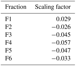

Figure 4Q1–50 and Q3–50 temporal patterns projected for temperature rise of 5 ∘C. Total rainfall of 160 mm over 24 h with each fraction representing accumulated rain for 4 h periods.
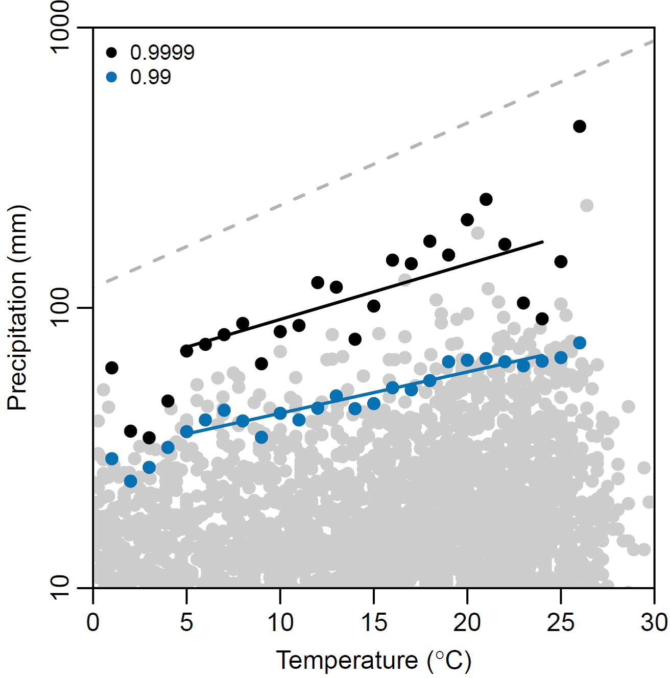
Figure 5Scaling total volume of rainfall with temperature for Minneapolis (1901–2014 daily rainfall). Grey dots are rainfall temperature pairs and the colored dots are the extreme percentiles. The grey dashed line represents a scaling of 7 %.
As the slopes in Fig. 3 and factors in Table 3 show, only the first fraction scaled positively, which means that the 4 h that included the highest amount of rainfall scale up while the remaining rainfall fractions scale down. The results are consistent with “invigorating storm dynamics” (Lenderink and van Meijgaard, 2008; Trenberth, 2011; Wasko and Sharma, 2015; Wasko et al., 2016b) resulting in a less uniform, more intense storm. The percentage adjustments were normalized to make sure that total rainfall amount did not change from the current value of 160 mm in 24 h. Figure 4 presents (Q1–50 and Q3–50 shown as an example) the changes in the temporal patterns when the scaling percentages calculated above are applied. Figure 4 illustrates the change to the highest peak rainfall rate and the decrease in the rest of the rainfall fractions. Similar scaling was applied for all six temporal patterns that were used in the H–H modeling analysis. As an additional verification, a similar analysis was completed for two neighboring locations (Sioux Falls, South Dakota, and Milwaukee, Wisconsin). The fraction and volume scaling results for both Sioux Falls and Milwaukee were consistent with those discussed in this paper.
Figure 5 presents the precipitation volume–temperature pairs, the extreme percentiles generated based on the temperature bins, as well as the resulting scaling for the 24 h rainfalls. The daily total rainfall of 160 mm fell into the 99.99th percentile based on a cursory ranking of the daily precipitation data. Hence, the 99.99th percentile 4.7 % scaling was selecting for the 24 h volume. This is broadly consistent with Utsumi et al. (2011) and Wasko et al. (2016a) who present scaling between 2 and 5 % for the central north of the United States for the 99th percentile and throughout Australia and less than the scaling found by Mishra et al. (2012) who used hourly precipitation, which is consistent with the expectation that shorter duration extremes have greater scaling (Hardwick Jones et al., 2010a; Panthou et al., 2014; Wasko et al., 2015). This value also appears to be consistent both with historical trends and climate change projections. Barbero et al. (2017) looked at a nonstationary extreme value analysis and found a sensitivity of approximately 7 % ∘C−1 for a nonstationary Theil–Sen estimator for North America. Globally, Westra et al. (2013a) found historical trends have global sensitivity between 5.9 and 7.7 % ∘C−1. However, Kharin et al. (2013) reported an approximately 4 % sensitivity over land globally from the CMIP5 model results with a range of 2.5–5 % for the United States. Relative to the literature stated above we believe our projections are consistent with the available evidence regarding precipitation change.
This 4.7 % scaling converts to an approximately 20 % increase in the volume of rainfall in a 24 h period for a 5∘ increase. Applying the 20 % increase to the 160 mm in 24 h gives a rainfall depth of 208 mm in 24 h. Coincidentally, 208 mm (∼ 210 mm) in 24 h is the upper margin of the 90 % confidence interval for the 160 mm event based on the margin provided in NOAA Atlas 14.
5.2 Flood depth response to temporal patterns and total rainfall variability
The H–H model was run for the 18 different combinations of rainfall volumes and temporal patterns. Results are presented for the five reference locations throughout the watershed representing different land use types that are typical in a developed area as described in Table 2. The selection of the reference points essentially provides results at different sub-catchments, or different sub-models. These sub-models show the variation in catchment response to runoff generated by a variety of land use types as well as changes in how the flows move through the different storm water infrastructure.
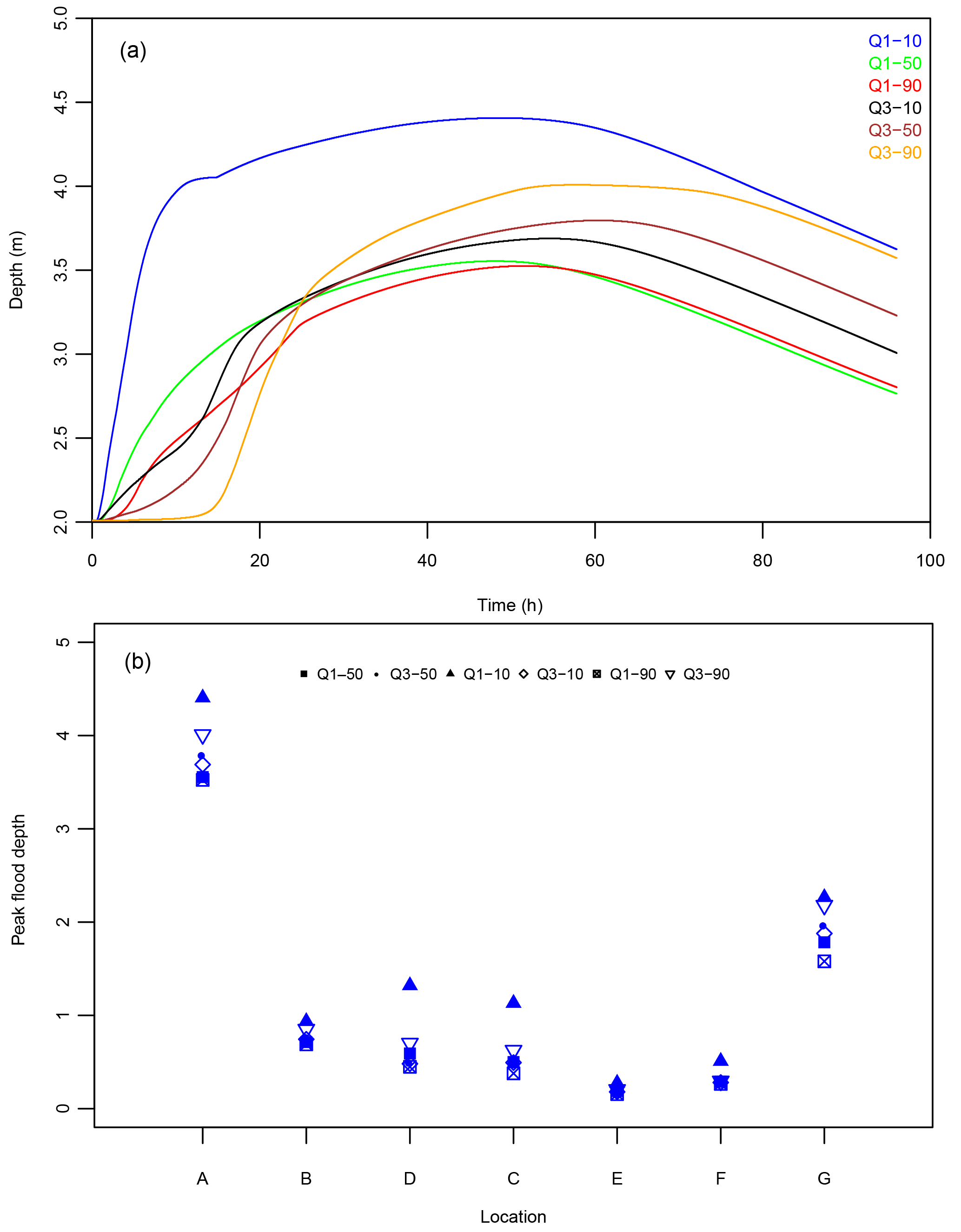
Figure 6(a) Depth over time at Wilmes Lake (location A), which is the downstream regional reference point in Fig. 1. Depth vs. time curves are plotted for 160 mm of total rainfall over 24 h with the six temporal patterns. Panel (b) presents the variation of peak flood depth (m) at reference locations throughout the watershed (refer to Table 1) with variation of temporal patterns for a total of 160 mm of rainfall over 24 h.
Figure 6a shows the depth/time curve at Wilmes Lake (location A), which is the main regional collection point and the downstream end of the model. Each curve represents change in depth vs. time for the six temporal patterns distributing the same total rainfall volume of 160 mm. The differences in shape, peak flood depth and the time to peak illustrate the variability in catchment response that can result purely due to variation in rainfall pattern during a storm event. A striking result is the approximately 1.3 m variation in flood depth at Wilmes Lake purely due to variation in how the rain falls within the duration of the storm. The highest flood depth curve is a result of the most intense storm event pattern, which is the Q1–10 distribution. The depth at Wilmes Lake rises quickly during the Q1–10 event but the peak flood depth still occurs within the 40–60 h band, similar to the other rainfall patterns. The high intensity of the Q1–10 pattern can overwhelm local conveyance and storage structures, resulting in overflows that flush down to the low-lying areas rapidly, causing the water level at the lake to rise. Note that the next highest peak flood level results from the Q3 pattern, which has the majority of the precipitation loaded in the latter half of the storm event. Comparison of the total runoff volume generated during each model run for the catchment between Q1–50 and Q3–50 temporal patterns shows a 9.5 % increase (refer to Table S4) for the same 50-year (160 mm in 24 h) storm event. A third quartile rainfall pattern can result in higher runoff volume as the soil saturates and infiltration rates are reduced and can cause worse flooding as local storage structures and ponds fill up by the time the bulk of the storm occurs. The results for the Q-3 patterns suggest that regional storage facilities such as Wilmes Lake within the SWWD are more sensitive to the runoff volume than the instantaneous peak flow rate, and thereby more sensitive to end-loaded temporal patterns during storms.
Figure 6b illustrates the same type of variation of peak flood depth due purely to the different temporal patterns at all of the reference points. Locations A, C, D and G average about 1 m in peak flood depth variation. When considering that the typical freeboard (the added elevation above the base flood elevation) used in the United States when setting the lowest open elevations for structures is 0.65 m, a 1 m variation in peak flood elevation is significant. As described in Table 1, the land use within the subcatchment that drains to location B is rural with local natural storage, whereas locations C and D have commercial land use with higher impervious land cover. This difference in land cover can explain why the variability in peak flood depth relative to changes in temporal patterns is lower at approximately 0.5 m and suggests that catchments with higher impervious surfaces have a higher sensitivity to rainfall patterns. Additionally, location F is within the storm sewer system, which suggests that variation in flow rates, or peak runoff from a catchment, does not always translate to higher variation in flood depths.
The depth vs. time curves in Fig. 6a also illustrate the value of including detailed hydraulic routing in the modeling analysis. As an example, the curves for Q1–10 and Q3–90 patterns show the difference of catchment response due to a high-intensity rainfall event that results in an initial peak flood depth resulting from overflows followed by the lagged response of the volume accumulation compared to the scenario of higher volume of runoff due to saturated soils. The variability in how the catchment responds to different temporal patterns is consistent with studies by Ball (1994) and Lambourne and Stephenson (1987). Though these studies focused primarily on the hydrologic aspect of the modeling and peak flow rates and volumes, the variation in catchment response to changes in “how it rains” is similar. The current study has the added benefit of detailed hydraulic routing and it is reasonable to assume that using only hydrologic routing, which is more common in current literature, would not have captured some of the detailed environmental hydraulics that can lead to better flood estimates in developed environments.
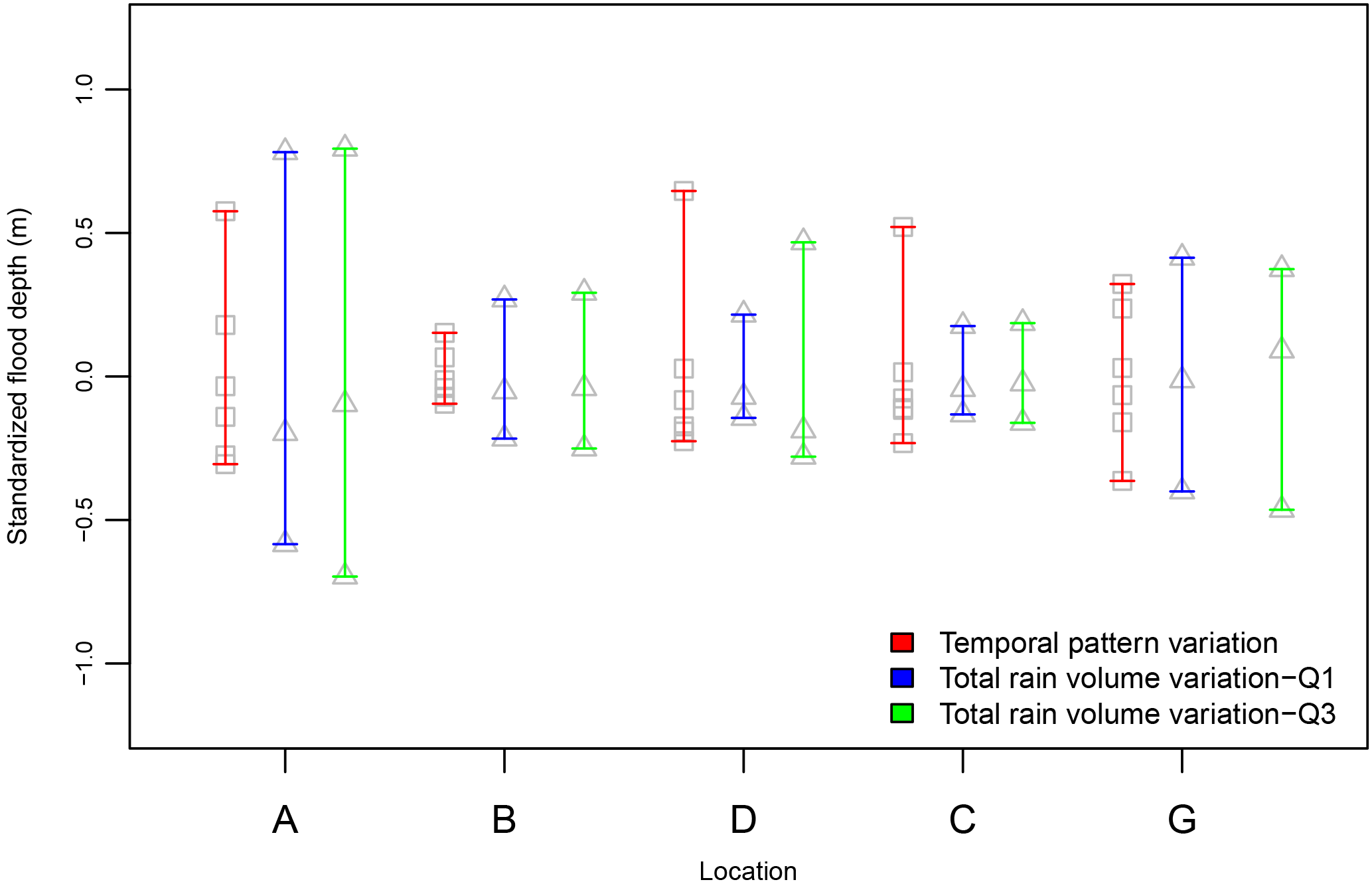
Figure 7Comparison of total volume of rainfall and temporal patterns' variability impact on peak flood depth. Flood depth variation due to the six different temporal patterns with 160 mm of rain compared to 110, 160 and 210 mm of total rainfall over 24 h distributed over Q1–50 and Q3–50 temporal patterns. Flood depths were standardized by subtracting the mean at each location for ease of comparison.
One of the primary questions that we set out to answer was the comparison of how it rains vs. how much it rains. For clarification, how it rains refers to the variation of temporal patterns during a storm event with the total rainfall volume within the 24 h held constant. The term “how much it rains” refers to different volumes of total rainfall within 24 h for each storm event with the temporal pattern held constant. Figure 7 makes the direct comparison between the variations of peak flood depth between how it rains and how much it rains. The range in peak depths at the reference locations indicates how the different catchments respond to variability in storm volume and pattern.
Comparison of the range of peak flood depths at locations C and D indicates a higher sensitivity to variation in how it rains as opposed to changes in how much it rains. Conversely, locations A, B and G indicate a higher range in flood depths due to changes in total rainfall volume, or how much it rains compared to changes in temporal patterns, or how it rains. Even though one can note that locations C and D receive runoff from catchments that have a majority of higher impervious land use relative to other locations, the number of data points does not allow for a statistically significant comparison of the sensitivity of impervious percentages in land use to the difference in how it rains vs. how much it rains. But it is important to note the consistency in the range of results across all the locations and the fact that how it rains has as much of an impact in the peak flood depths as how much it rains. The results in Fig. 7 clearly answer the first question presented in the introduction that temporal patterns of storms are as important as the total volume of rainfall during a storm in watershed response and flood estimation.
The results presented in Figs. 6 and 7 show that temporal patterns, or how it rains, add a degree of variability and have a significant contribution to the overall uncertainty in H–H modeling results. This is especially a concern given the evidence to date that systematic change is occurring in rainfall patterns across climate zones, making them more intense and impactful in derived flood estimations (Wasko and Sharma, 2015). The added variability has implications on the already complex nature of properly accounting for uncertainty in flood forecasts or the impacts of climate change in future flooding conditions, which can in turn have implications on how society will accept the socio-economic impacts of adaption as previously mentioned. Hence, careful consideration of how it rains and changes in how it rains have to be included in any H–H modeling framework along with the current typical practice of modeling how much it rains.
5.3 Impact of applying temperature scaling to temporal patterns and rainfall volume on flood depths
Figure 8 compares the results for projected temporal patterns with results from the base simulation. Both scenarios are based on the 50-year return period event, which consists of 160 mm of total rain distributed over the six base and projected temporal patterns. The results shown in Fig. 8 are variation of the peak flood depth around the mean of the results from the base condition models. In other words, the results were standardized by subtracting the mean of the base conditions from the results at each location.
As expected, the highest flood depth results from the Q1–10 pattern for both current and scaled conditions. But the results at the highest depths show little change due to temperature scaling of the Q1–10 pattern. The Q1–10 pattern is an extremely high-intensity event, with the majority of the rainfall occurring in the first fraction of the event. Applying the scaling percentages to this fraction makes minimal changes to the overall pattern of rainfall, resulting in no appreciable change in peak flood depths. If we take the extreme Q1–10 event out of consideration, one can say that qualitatively, there is an increasing trend in flood depths due to changes in the projected temporal patterns. The important fact is that these plots are based on the same total rainfall volume of 160 mm. The moderate increasing trend in the results is purely due to the projected temporal patterns. As discussed previously, location B represents a more rural-type catchment and shows less sensitivity to changes in rainfall patterns.
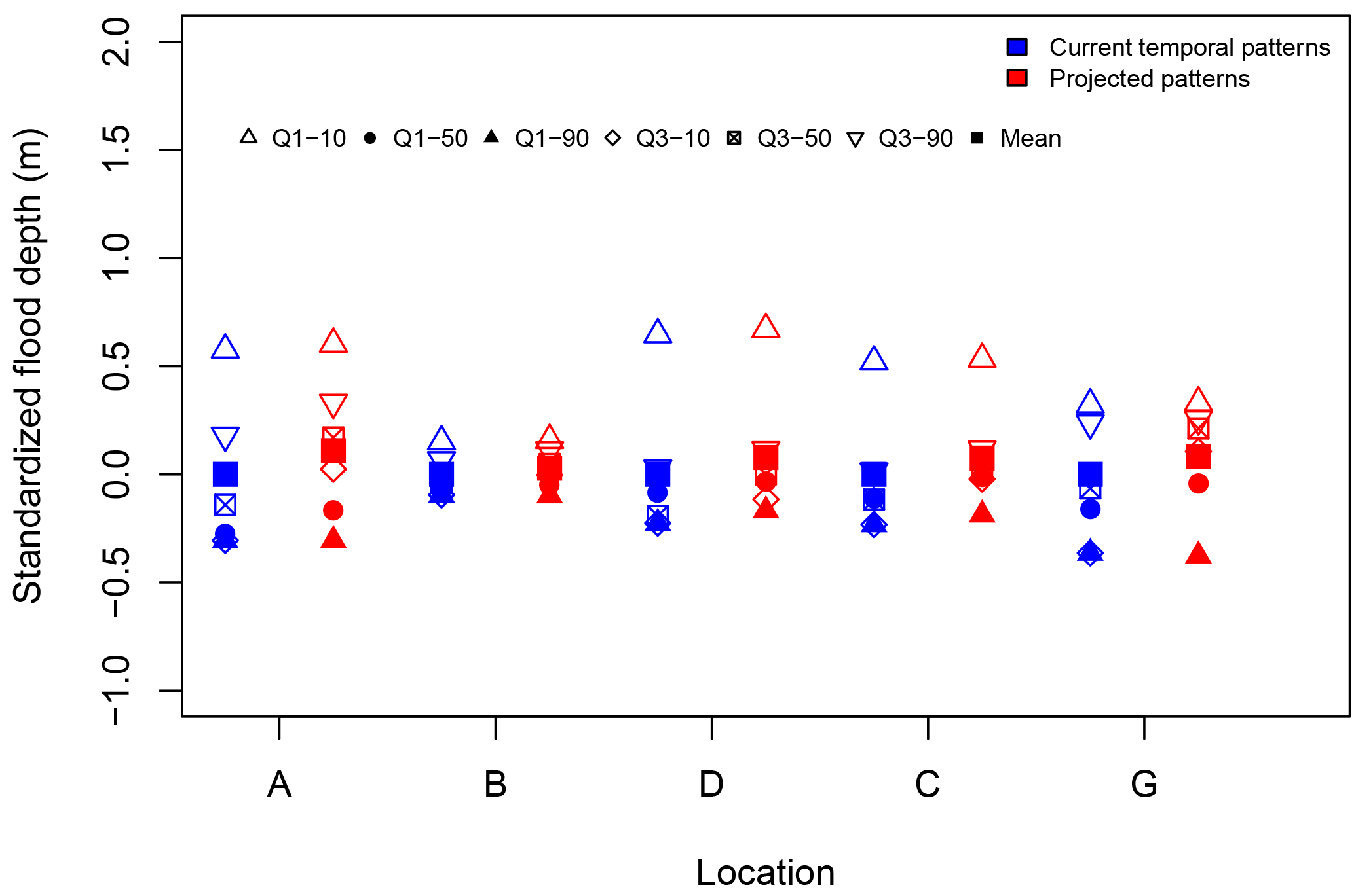
Figure 8Impact of rise in temperature on the peak flood depth variation at reference locations within the watershed when scaling is applied only to temporal patterns. The peak flood depths at each reference point are based on 160 mm of total rain distributed over the six temporal patterns used. Temperature scaling (T∕S) for the temporal patterns is based on scaling fractions presented in Fig. 3. Flood depths were standardized by subtracting the mean from the base simulations presented in Fig. 6 for each location. The mean flood depth is shown as solid squares.
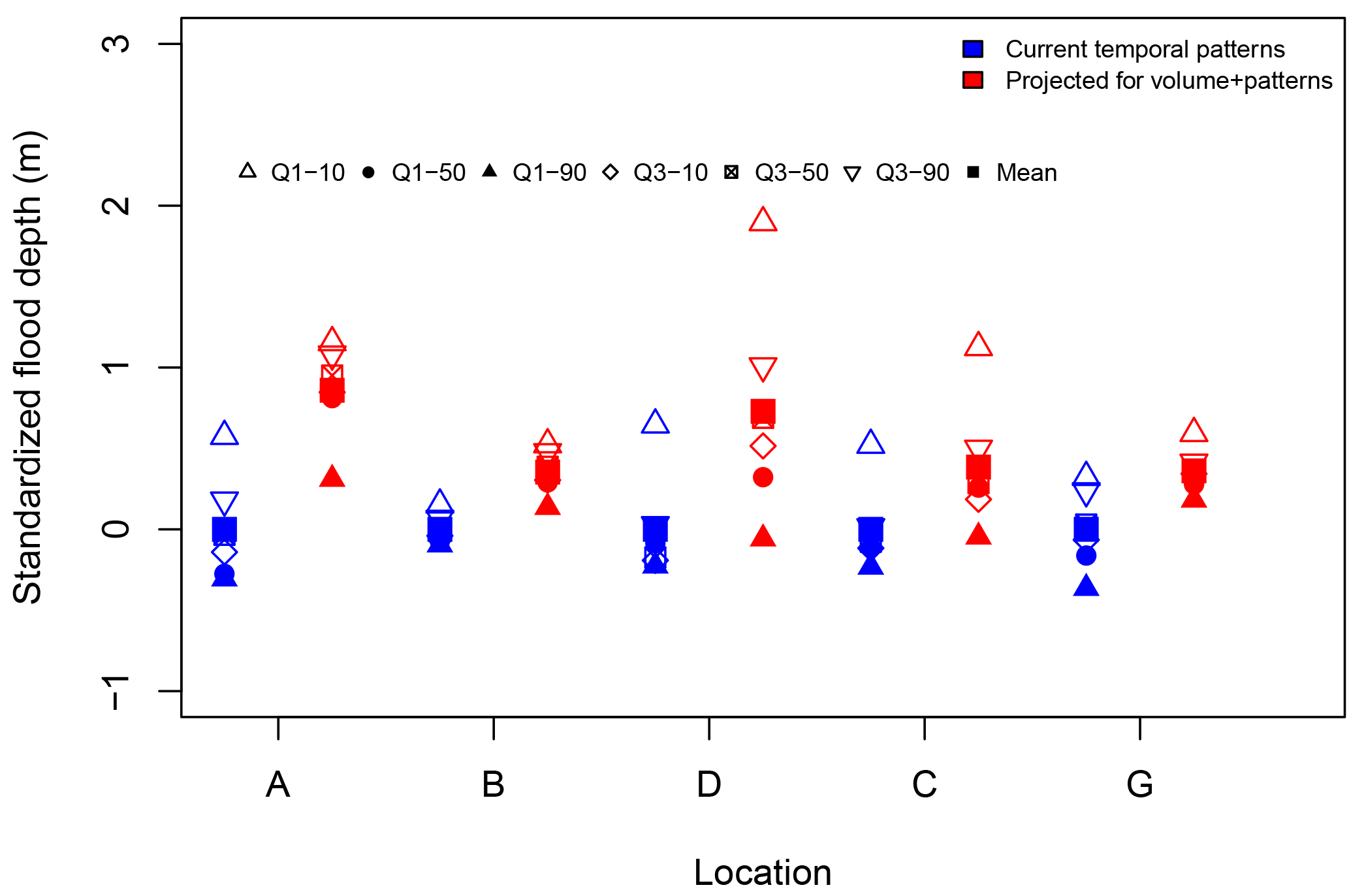
Figure 9Impact of rise in temperature on the peak flood depth variation at reference locations within the watershed, when scaling is applied to both rainfall volume and temporal pattern. The peak flood depths at each reference point are based on 210 mm of total rain distributed over the six temporal patterns used. Flood depths were standardized by subtracting the mean from the base simulations presented in Fig. 6 for each location. The mean flood depth is shown as solid squares.
Figure 9 shows the same comparison as in Fig. 8 when temperature scaling is applied to both the temporal pattern and rainfall volume. Hence Fig. 9 presents the cumulative impacts of temperature scaling to the base conditions. As in Fig. 8, the results in Fig. 9 show the variation of results for both scenarios around the mean of the base condition flood depth at each location.
As expected, a substantial increase in flood risk is seen when the cumulative impacts of changes to temporal pattern and increase in precipitation volume due to temperature rise are modeled. The mean flood depth is outside the upper margin of the highest flood depth for base conditions except at the business park (C). The business park location (C) comes close to meeting this threshold as well. The mean flood depth at Wilmes Lake (A) increases by approximately 1 m, which translates to a significant increase in the extent of flooding. The biggest change due to cumulative impacts occurs at the upstream location (B) where previously, when only the temporal patterns were scaled, minimal impact was shown. The increase in flood depth at the reference locations due to changes to temporal patterns alone ranges from 1 to 35 %, while the cumulative impacts increase flood depth from 10 % to as much as 170 %. These results are similar to Zhou et al. (2018) who projected a 52 % increase in urban flooding for an RCP8.5 scenario in China. When considering all the nodes in the model, the average increase in flood depth due only to changes in temporal patterns was 6 %. The average increase in flood depth throughout the entire model due to cumulative impacts of both changes to temporal pattern and rainfall volume is 37 %. The percentage increase (Table S2) shows that there is a significant impact on overall flood risk throughout the catchment and that it is not only confined to the reference points that have been discussed in detail in this paper. These results clearly show the increasing trend along with the significant variability in flood risk in developed environments.
Additionally, the range of the results and hence the overall variability has increased at the commercial and business park area (C, D) locations when compared to Fig. 8. But this change in the range is not consistent throughout the catchment. The higher intensity and the larger total volume of rainfall overwhelm the existing infrastructure with much larger surface overflows in different ways depending on the site and extent. Also, the amount of increase in the flood depths can change at different locations as the flooding increases. The changes to the range of depths as seen in Fig. 9 suggest that quantifying and accounting for uncertainty in flood forecasts will become more complex for future climates.
The use of detailed hydrologic and hydraulic modeling provides some of the nuances in catchment response that add important details to the results and our understanding of the impacts of temporal patterns on flood risk, such as that higher intensity rainfall does not always result in a higher flood risk. The variation of reference locations selected for this study provides a reasonable assessment of how the flows interact with the physical features of the catchment and how the results differ based on the location and features. This study clearly shows the sensitivity of the catchment to variation in how it rains, in particular the areas that are more impacted by volume as opposed to flow rate. Explicitly including intensification of rainfall patterns and volume due to climate change along with detailed H–H modeling to assess the variability in catchment response makes this study unique among available literature. The methodology presented here is universally applicable and the benefits of correctly designing infrastructure are likely to far outweigh the cost of the added effort, even in industry applications.
The significance of temporal patterns and how climate change impacts on rainfall patterns affect flooding in developed environments was investigated using detailed hydrologic and hydraulic modeling. Climate change impacts were undertaken by projecting historical precipitation–temperature sensitivities on storm volumes and temporal patterns. The following conclusions can be drawn from the results presented.
-
The response of a complex catchment is sensitive to variability in rainfall temporal patterns. The flood depths varied in excess of 1 m at Wilmes Lake when different temporal patterns were used with a constant volume of precipitation.
-
The variability of peak flood depth due to temporal pattern had similar magnitude when compared to variability due to total rainfall volume, which clearly shows that the temporal pattern of rainfall, or how it rains is as important as the volume of rainfall or how much it rains for the purposes of H–H modeling.
-
Temporal patterns add a quantifiable variability to the results generated in H–H modeling and need to be carefully considered when presenting results and associated uncertainties.
-
The temporal patterns intensified when scaled based on estimated temperature increases due to climate change.
-
A 1 to 35 % increase in flood depth resulted when the scaled temporal patterns were used in the H–H model, suggesting an increase in potential flood risk purely due to changes in how it rains as a result of climate change impacts.
-
A 10 to 170 % increase in flood depth resulted when the projected rainfall volume was added to the projected temporal patterns, which shows a substantial increase in flood risk as a result of climate change impacts on rainfall.
-
The variability of flood depth increased after temporal patterns and rainfall volumes were projected, suggesting that H–H modeling for future planning and design needs to give serious consideration to the aspects of variability of rainfall patterns as well as increases in rainfall amounts.
-
Regional storage facilities are sensitive to rainfall patterns that are loaded in the latter part of the storm duration, while extremely intense storms will cause flooding at all locations.
The effect of projected intensification of storms due to climate change impacts suggests that action needs to be taken promptly to prevent flood damage and possible loss of life. The most important point that can be derived from this study is that temporal patterns and storm volumes need to be adjusted to account for climate change when they are applied to models of future scenarios. The general application of H–H modeling analysis needs to adopt an ensemble approach rather than a single event model to consider the significant variability in rainfall patterns that can generate a substantial range in results in order to make a properly informed decision as demonstrated here.
The rainfall and temperature data for Minneapolis Airport and locations around the site were taken from https://www.ncdc.noaa.gov/cdo-web/. NOAA Atlas 14 Volume 8 is available at http://www.nws.noaa.gov/oh/hdsc/PF_documents/Atlas14_Volume8.pdf (Perica et al., 2013). Technical details of EPA SWMM can be found at https://www.epa.gov/water-research/storm-water-management-model-swmm.
The supplement related to this article is available online at: https://doi.org/10.5194/hess-22-2041-2018-supplement.
The authors declare that they have no conflict of interest.
The authors acknowledge and thank the South Washington Watershed District
(http://www.swwdmn.org) in Minnesota, United States, for providing the
model as well as the background data used for the analysis. We also
acknowledge financial support of the Australian Research Council.
Edited by: Louise Slater
Reviewed by: two anonymous referees
Adams, B. J. and Howard, C. D.: Design storm pathology, Can. Water Resour. J., 11, 49–55, 1986.
Adger, W. N., Agrawala, S., Mirza, M. M. Q., Conde, C., o'Brien, K., Pulhin, J., Pulwarty, R., Smit, B., and Takahashi, K.: Assessment of adaptation practices, options, constraints and capacity, Climate change 2007: Impacts, Adaptation and Vulnerability. Contribution of Working Group II to the Fourth Assessment Report of the Intergovernmental Panel on Climate Change, 2007, 717–743, 2007.
Adger, W. N., Dessai, S., Goulden, M., Hulme, M., Lorenzoni, I., Nelson, D. R., Naess, L. O., Wolf, J., and Wreford, A.: Are there social limits to adaptation to climate change?, Climatic Change, 93, 335–354, 2009.
Agilan, V. and Umamahesh, N.: Modelling nonlinear trend for developing non-stationary rainfall intensity–duration–frequency curve, Int. J. Climatol., 37, 1265–1281, 2017.
Alexander, L. V., Zhang, X., Peterson, T. C., Caesar, J., Gleason, B., Tank, A. M. G. K., Haylock, M., Collins, D., Trewin, B., Rahimzadeh, F., Tagipour, A., Kumar, K. R., Revadekar, J., Griffiths, G., Vincent, L., Stephenson, D. B., Burn, J., Aguilar, E., Brunet, M., Taylor, M., New, M., Zhai, P., Rusticucci, M., and Vazquez-Aguirre, J. L.: Global observed changes in daily climate extremes of temperature and precipitation, J. Geophys. Res.-Atmos., 111, 1–22, 2006.
Ali, H. and Mishra, V.: Contrasting response of rainfall extremes to increase in surface air and dewpoint temperatures at urban locations in India, Sci. Rep.-UK, 7, 1228, https://doi.org/10.1038/s41598-017-01306-1, 2017.
Ashley, R. M., Balmforth, D. J., Saul, A. J., and Blanskby, J.: Flooding in the future–predicting climate change, risks and responses in urban areas, Water Sci. Technol., 52, 265–273, 2005.
Ball, J. E.: The influence of storm temporal patterns on catchment response, J. Hydrol., 158, 285–303, 1994.
Barbero, R., Fowler, H. J., Lenderink, G., and Blenkinsop, S.: Is the intensification of precipitation extremes with global warming better detected at hourly than daily resolutions?, Geophys. Res. Lett., 44, 974–983, 2017.
Bisht, D. S., Chatterjee, C., Kalakoti, S., Upadhyay, P., Sahoo, M., and Panda, A.: Modeling urban floods and drainage using SWMM and MIKE URBAN: a case study, Nat. Hazards, 84, 749–776, 2016.
Cameron, D.: An application of the UKCIP02 climate change scenarios to flood estimation by continuous simulation for a gauged catchment in the northeast of Scotland, UK (with uncertainty), J. Hydrol., 328, 212–226, 2006.
Donat, M. G., Alexander, L. V., Yang, H., Durre, I., Vose, R., Dunn, R. J. H., Willett, K. M., Aguilar, E., Brunet, M., Caesar, J., Hewitson, B., Jack, C., Tank, A. M. G. K., Kruger, A. C., Marengo, J., Peterson, T. C., Renom, M., Rojas, C. O., Rusticucci, M., Salinger, J., Elrayah, A. S., Sekele, S. S., Srivastava, A. K., Trewin, B., Villarroel, C., Vincent, L. A., Zhai, P., Zhang, X., and Kitching, S.: Updated analyses of temperature and precipitation extreme indices since the beginning of the twentieth century: The HadEX2 dataset, J. Geophys. Res.-Atmos., 118, 2098–2118, 2013.
Doocy, S., Daniels, A., Murray, S., and Kirsch, T.: The Human impact of floods: a historical review of events 1980–2009 and systematic literature review, PLOS Current Disasters, 5, 1–29, 2013.
EPA: USA, Storm Water Management Model, 1–2, 2016.
Feyen, L., Barredo, J., and Dankers, R.: Implications of global warming and urban land use change on flooding in Europe, Water & Urban Development Paradigms-Towards an integration of engineering, design and management approaches, edited by: Feyen, J., Shannon, K., and Neville, M., 217–225, 2008.
Fowler, H. J., Blenkinsop, S., and Tebaldi, C.: Linking climate change modelling to impacts studies: recent advances in downscaling techniques for hydrological modelling, Int. J. Climatol., 27, 1547–1578, 2007.
Füssel, H. M.: Adaptation planning for climate change: concepts, assessment approaches, and key lessons, Sustain. Sci., 2, 265–275, 2007.
García-Bartual, R. and Andrés-Doménech, I.: A two-parameter design storm for Mediterranean convective rainfall, Hydrol. Earth Syst. Sci., 21, 2377–2387, https://doi.org/10.5194/hess-21-2377-2017, 2017.
Graham, L. P., Andréasson, J., and Carlsson, B.: Assessing climate change impacts on hydrology from an ensemble of regional climate models, model scales and linking methods – a case study on the Lule River basin, Climatic Change, 81, 293–307, 2007.
Hardwick Jones, R., Westra, S., and Sharma, A.: Observed relationships between extreme sub-daily precipitation, surface temperature, and relative humidity, Geophys. Res. Lett., 37, L22805, https://doi.org/10.1029/2010GL045081, 2010.
Hartmann, D. L., Klein Tank, A. M., Rusticucci, M., Alexander, L. V., Brönnimann, S., Charabi, Y. A. R., Dentener, F. J., Dlugokencky, E. J., Easterling, D. R., and Kaplan, A.: Climate Change 2013 the Physical Science Basis: Working Group I Contribution to the Fifth Assessment Report of the Intergovernmental Panel on Climate Change, 2013.
Hettiarachchi, S., Beduhn, R., Christopherson, J., and Moore, M.: Managing Surface Water for Flood Damage Reduction, World Water and Environmental Resources Congress 2005, Anchorage, Alaska, United States, https://doi.org/10.1061/40792(173)321, 15–19 May 2005.
Huff, F. A.: Time distribution of rainfall in heavy storms, Water Resour. Res., 3, 1007–1019, 1967.
IPCC: Climate Change 2014: Synthesis Report. Contribution of Working Groups I, II and III to the Fifth Assessment Report of the Intergovernmental Panel on Climate Change, edited by: Core Writing Team, Pachauri, R. K. and Meyer, L. A., IPCC, Geneva, Switzerland, 151 pp., 2014.
Kharin, V. V., Zwiers, F. W., Zhang, X., and Wehner, M.: Changes in temperature and precipitation extremes in the CMIP5 ensemble, Climatic Change, 119, 345–357, https://doi.org/10.1007/s10584-013-0705-8, 2013.
Lambourne, J. J. and Stephenson, D.: Model study of the effect of temporal storm distributions on peak discharges and volumes, Hydrolog. Sci. J., 32, 215–226, 1987.
Leander, R., Buishand, T. A., van den Hurk, B. J. J. M., and de Wit, M. J. M.: Estimated changes in flood quantiles of the river Meuse from resampling of regional climate model output, J. Hydrol., 351, 331–343, 2008.
Lenderink, G. and Attema, J.: A simple scaling approach to produce climate scenarios of local precipitation extremes for the Netherlands, Environ. Res. Lett., 10, 085001, https://doi.org/10.1088/1748-9326/10/8/085001, 2015.
Lenderink, G., Mok, H. Y., Lee, T. C., and van Oldenborgh, G. J.: Scaling and trends of hourly precipitation extremes in two different climate zones – Hong Kong and the Netherlands, Hydrol. Earth Syst. Sci., 15, 3033–3041, https://doi.org/10.5194/hess-15-3033-2011, 2011.
Lenderink, G. and van Meijgaard, E.: Increase in hourly precipitation extremes beyond expectations from temperature changes, Nat. Geosci., 1, 511–514, 2008.
Mamo, T. G.: Evaluation of the Potential Impact of Rainfall Intensity Variation due to Climate Change on Existing Drainage Infrastructure, J. Irrig. Drain. Eng., 141, 1–7, 2015.
Manola, I., van den Hurk, B., De Moel, H., and Aerts, J.: Future extreme precipitation intensities based on historic events, Hydrol. Earth Syst. Sci. Discuss., https://doi.org/10.5194/hess-2017-227, in review, 2017.
Maraun, D., Wetterhall, F., Ireson, A. M., Chandler, R. E., Kendon, E. J., Widmann, M., Brienen, S., Rust, H. W., Sauter, T., Themeßl, M., Venema, V. K. C., Chun, K. P., Goodess, C. M., Jones, R. G., Onof, C., Vrac, M., and Thiele-Eich, I.: Precipitation downscaling under climate change: Recent developments to bridge the gap between dynamical models and the end user, Rev. Geophys., 48, RG3003, https://doi.org/10.1029/2009RG000314, 2010.
Merz, B., Kreibich, H., Schwarze, R., and Thieken, A.: Review article “Assessment of economic flood damage”, Nat. Hazards Earth Syst. Sci., 10, 1697–1724, https://doi.org/10.5194/nhess-10-1697-2010, 2010.
Milly, P., Julio, B., Malin, F., Robert, M., Zbigniew, W., Dennis, P., and Ronald, J.: Stationarity is dead, Ground Water News & Views, 4, 6–8, 2007.
Mishra, V., Wallace, J. M., and Lettenmaier, D. P.: Relationship between hourly extreme precipitation and local air temperature in the United States, Geophys. Res. Lett., 39, 1–7, 2012.
Mockus, V., Merkel, W. H., Moody, H., Woodward, D. E., Hoeft, C. C., and Quan, Q. D.: National Engineering Handbook Chapter 4, Storm Rainfall Depth and Distribution, 2015.
Molnar, P., Fatichi, S., Gaál, L., Szolgay, J., and Burlando, P.: Storm type effects on super Clausius–Clapeyron scaling of intense rainstorm properties with air temperature, Hydrol. Earth Syst. Sci., 19, 1753–1766, https://doi.org/10.5194/hess-19-1753-2015, 2015.
Nguyen, V. T., Desramaut, N., and Nguyen, T. D.: Optimal rainfall temporal patterns for urban drainage design in the context of climate change, Water Sci. Technol., 62, 1170–1176, 2010.
Packman, J. and Kidd, C.: A logical approach to the design storm concept, Water Resour. Res., 16, 994–1000, 1980.
Panthou, G., Mailhot, A., Laurence, E., and Talbot, G.: Relationship between surface temperature and extreme rainfalls: A multi-time-scale and event-based analysis, J. Hydrometeorol., 15, 1999–2011, 2014.
Perica, S., Martin, D., Pavlovic, S., Roy, I., St. Laurent, M., Trypaluk, C., Unruh, D., Yekta, M., and Bonnin, G.: NOAA Atlas 14 precipitation- frequency Atlas of the United States, Volume 8, Version 2.0, Midwestern States (Colorado, Iowa, Kansas, Michigan, Minnesota, Missouri, Nebraska, North, Dakota, Oklahoma, South Dakota, Wisconsin), NOAA, National Weather Service, Silver Spring, MD, 2013 (data available at: http://www.nws.noaa.gov/oh/hdsc/PF_documents/Atlas14_Volume8.pdf).
Peters, G. P., Andrew, R. M., Boden, T., Canadell, J. G., Ciais, P., Le Quéré, C., Marland, G., Raupach, M. R., and Wilson, C.: The challenge to keep global warming below 2 ∘C, Nat. Clim. Change, 3, 4–6, https://doi.org/10.1038/nclimate1783, 2013.
Pilgrim, D., Kennedy, M., Rowbottom, I., Cordery, I., Canterford, R., and Turner, L.: Section 2 – Temporal Patterns of Rainfall Burst, in: Australian Rainfall and Runoff – A Guide to Flood Estimation, Institute of Engineers Australia, 1997.
Prudhomme, C. and Davies, H.: Assessing uncertainties in climate change impact analyses on the river flow regimes in the UK. Part 2: future climate, Climatic Change, 93, 197–222, 2009.
Prudhomme, C., Reynard, N., and Crooks, S.: Downscaling of global climate models for flood frequency analysis: where are we now?, Hydrol. Process., 16, 1137–1150, 2002.
Raff, D. A., Pruitt, T., and Brekke, L. D.: A framework for assessing flood frequency based on climate projection information, Hydrol. Earth Syst. Sci., 13, 2119–2136, https://doi.org/10.5194/hess-13-2119-2009, 2009.
Rivard, G.: Design Storm Events for Urban Drainage Based on Historical Rainfall Data: A Conceptual Framework for a Logical Approach, Journal of Water Management Modeling, Rl91-12, 187–199, 1996.
Sandink, D.: Urban flooding and ground-related homes in Canada: an overview, J. Flood Risk Manag., 9, 208–223, https://doi.org/10.1111/jfr3.12168, 2015.
Schreider, S. Y., Smith, D. I., and Jakeman, A. J.: Climate Change Impacts on Urban Flooding, Climatic Change, 47, 91–115, 2000.
Seneviratne, S. I., Nicholls, N., Easterling, D., Goodess, C. M., Kanae, S., Kossin, J., Luo, Y., Marengo, J., McInnes, K., and Rahimi, M.: Changes in climate extremes and their impacts on the natural physical environment, in: Managing the risks of extreme events and disasters to advance climate change adaptation, Cambridge University Press, Cambridge, UK, and New York, NY, USA, 2012.
Sillmann, J., Kharin, V., Zwiers, F., Zhang, X., and Bronaugh, D.: Climate extremes indices in the CMIP5 multimodel ensemble: Part 2. Future climate projections, J. Geophys. Res.-Atmos., 118, 2473–2493, 2013.
Singh, V. P. and Woolhiser, D. A.: Mathematical modeling of watershed hydrology, J. Hydrol. Eng., 7, 270–292, 2002.
Smith, B. K., Smith, J., and Baeck, M. L.: Flash Flood–Producing Storm Properties in a Small Urban Watershed, J. Hydrometeorol., 17, 2631–2647, 2016.
Sørup, H. J. D., Christensen, O. B., Arnbjerg-Nielsen, K., and Mikkelsen, P. S.: Downscaling future precipitation extremes to urban hydrology scales using a spatio-temporal Neyman–Scott weather generator, Hydrol. Earth Syst. Sci., 20, 1387–1403, https://doi.org/10.5194/hess-20-1387-2016, 2016.
Thodsen, H.: The influence of climate change on stream flow in Danish rivers, J. Hydrol., 333, 226–238, 2007.
Trenberth, K. E.: Changes in precipitation with climate change, Clim. Res., 47, 123–138, 2011.
United Nations, Department of Economic and Social Affairs, Population Division: World Urbanization Prospects: The 2014 Revision, Highlight, 2014, 2014.
Utsumi, N., Seto, S., Kanae, S., Maeda, E. E., and Oki, T.: Does higher surface temperature intensify extreme precipitation?, Geophys. Res. Lett., 38, L16708, https://doi.org/10.1029/2011GL048426, 2011
van Pelt, S. C., Kabat, P., ter Maat, H. W., van den Hurk, B. J. J. M., and Weerts, A. H.: Discharge simulations performed with a hydrological model using bias corrected regional climate model input, Hydrol. Earth Syst. Sci., 13, 2387–2397, https://doi.org/10.5194/hess-13-2387-2009, 2009.
Wasko, C. and Sharma, A.: Quantile regression for investigating scaling of extreme precipitation with temperature, Water Resour. Res., 50, 3608–3614, 2014.
Wasko, C. and Sharma, A.: Steeper temporal distribution of rain intensity at higher temperatures within Australian storms, Nat. Geosci., 8, 527–529, 2015.
Wasko, C. and Sharma, A.: Continuous rainfall generation for a warmer climate using observed temperature sensitivities, J. Hydrol., 544, 575–590, 2017.
Wasko, C., Sharma, A., and Johnson, F.: Does storm duration modulate the extreme precipitation-temperature scaling relationship?, Geophys. Res. Lett., 42, 8783–8790, 2015.
Wasko, C., Parinussa, R., and Sharma, A.: A quasi-global assessment of changes in remotely sensed rainfall extremes with temperature, Geophys. Res. Lett., 43, 12659–12668, https://doi.org/10.1002/2016GL071354, 2016a.
Wasko, C., Sharma, A., and Westra, S.: Reduced spatial extent of extreme storms at higher temperatures, Geophys. Res. Lett., 43, 4026–4032, 2016b.
Westra, S., Alexander, L. V., and Zwiers, F. W.: Global Increasing Trends in Annual Maximum Daily Precipitation, J. Climate, 26, 3904–3918, 2013a.
Westra, S., Evans, J. P., Mehrotra, R., and Sharma, A.: A conditional disaggregation algorithm for generating fine time-scale rainfall data in a warmer climate, J. Hydrol., 479, 86–99, 2013b.
Wilks, D. S.: Use of stochastic weathergenerators for precipitation downscaling, Wiley Interdisciplinary Reviews, Climate Change, 1, 898–907, 2010.
Willems, P., Arnbjerg-Nielsen, K., Olsson, J., and Nguyen, V. T. V.: Climate Change impact assessment on urban rainfall extremes and urban drainage: Methods and shortcomings, Atmos. Res., 103, 106–118, 2012.
Woldemeskel, F. M., Sharma, A., Mehrotra, R., and Westra, S.: Constraining continuous rainfall simulations for derived design flood estimation, J. Hydrol., 542, 581–588, 2016.
Zhou, X., Bai, Z., and Yang, Y.: Linking trends in urban extreme rainfall to urban flooding in China, Int. J. Climatol., 37, 4586–4593, https://doi.org/10.1002/joc.5107, 2017.
Zhou, Q., Leng, G., and Huang, M.: Impacts of future climate change on urban flood volumes in Hohhot in northern China: benefits of climate change mitigation and adaptations, Hydrol. Earth Syst. Sci., 22, 305–316, https://doi.org/10.5194/hess-22-305-2018, 2018.
Zope, P. E., Eldho, T. I., and Jothiprakash, V.: Impacts of land use–land cover change and urbanization on flooding: A case study of Oshiwara River Basin in Mumbai, India, CATENA, 145, 142–154, 2016.
Zoppou, C.: Review of urban storm water models, Environ. Modell. Softw., 16, 195–231, 2001.