the Creative Commons Attribution 4.0 License.
the Creative Commons Attribution 4.0 License.
 | 02 Jun 2022
Evaluation of obstacle modelling approaches for resource assessment and small wind turbine siting: case study in the northern Netherlands
Lindsay M. Sheridan
Patrick Conry
Dimitrios K. Fytanidis
Dmitry Duplyakin
Sagi Zisman
Nicolas Duboc
Matt Nelson
Rao Kotamarthi
Rod Linn
Marc Broersma
Timo Spijkerboer
Heidi Tinnesand
Growth in adoption of distributed wind turbines for energy generation is significantly impacted by challenges associated with siting and accurate estimation of the wind resource. Small turbines, at hub heights of 40 m or less, are greatly impacted by terrestrial obstacles such as built structures and vegetation that can cause complex wake effects. While some progress in high-fidelity complex fluid dynamics (CFD) models has increased the potential accuracy for modelling the impacts of obstacles on turbulent wind flow, these models are too computationally expensive for practical siting and resource assessment applications. To understand the efficacy of available models in situ, this study evaluates classic and commonly used methods alongside new state-of-the-art lower-order models derived from CFD simulations and machine learning approaches. This evaluation is conducted using a subset of an extensive original dataset of measurements from more than 300 operational wind turbines in the northern Netherlands. The results show that data-driven methods (e.g. machine learning and statistical modelling) are most effective at predicting production at real sites with an average error in annual energy production of 2.5 %. When sufficient data may not be available de novo to support these data-driven approaches, models derived from high-fidelity simulations show promise and reliably outperform classic methods. On average these models have 6.3 %–11.5 % error compared with 26 % for classic methods and 27 % baseline error for reanalysis data without obstacle correction. While more performant on average, these methods are also sensitive to the quality of obstacle descriptions and reanalysis inputs.
- Article
(5061 KB) - Full-text XML
- BibTeX
- EndNote


Distributed wind (DW) energy constitutes a small but growing market with a total global installed capacity estimated at approximately 1.8 GW (Orrell et al., 2021). As compared with their utility-scale counterparts, small wind turbines provide significant opportunity to diversify energy production and address a market niche not otherwise served, since they are particularly well suited to industrial, agricultural, and campus-level installations. Despite their significant potential as a component of a larger distributed energy resource (DER) portfolio, adoption of small wind is practically hindered by a number of challenges including project costs, availability of incentives, and confidence in the underlying technologies. Confidence, in particular, is strongly impacted by the practical accuracy in the prediction of energy production at a site of development interest (Fields et al., 2016). Yet, accurate energy production estimates can only be obtained by predicting the available wind resource. While large-scale wind plants can afford to perform detailed observation-driven wind resource and site assessments, small-scale wind projects typically rely on less-expensive use models and assessment tools to survey the energy production potential due to lower financial scope of anticipated projects. While the dependence on models is greater, the challenge to model the resource accurately is also significantly higher: small wind turbines are more greatly impacted by turbulence and wake effects from surrounding terrestrial obstacles such as buildings, trees, and vegetation (Drew et al., 2015).
The state of the art in assessment of obstacle influence on downwind wind fields for small-wind siting and resource assessment is characterized by the usage of tools that provide a mixture of analytical modelling and heuristic estimation (Poudel et al., 2019). The effect of isolated obstacles on the flow field structure has been studied in the past both experimentally (Schofield and Logan, 1990; Martinuzzi and Tropea, 1993; Snyder and Lawson, 1994; Hussein and Martinuzzi, 1996) and numerically (among others Lakehal and Rodi, 1997; Krajnović et al., 1999; Yakhot et al., 2006a, b). Velocity data from such studies can be used to approximate the effect of buildings on wind velocity profiles in the wake of isolated obstacles. Analytical models from the literature (Robins and Apsley, 2021; Counihan et al., 1974; Kothari et al., 1980; Peterka et al., 1985) have also been developed for the case of isolated cubes with zero wind angle of attack (conditions where wind approached the building perpendicular to one of its sides). Additionally, Perera (1981) used data from wind tunnel experiments and developed a model suitable to predict the velocity deficit at the wake of an infinitely long obstacle when the winds are perpendicular to the length of the obstacle.
As a potential compromise between high-fidelity solutions that are too computationally intense for non-expert use, such as large-eddy simulations (LES; Castro et al., 2017; Bieringer et al., 2021), and fitted models derived from isolated experimental campaigns, lower-fidelity computational fluid dynamics (CFD) models have been applied to more complex obstacle geometries to solve flow patterns in urban areas (Tominaga and Stathopoulos, 2013). Among these models are Reynolds-averaged Navier–Stokes (RANS; Bruse and Fleer, 1998; Gowardhan et al., 2011) modelling approaches, which while computationally faster, do not capture the physics at all scales relevant for urban flow and turbulence modelling. Although there have been recent demonstrations (Bierenger et al., 2021) of LES running ∼100 times faster when using graphical processing unit (GPU) approaches than when using the traditional central processing unit (CPU), the expertise required to set up such models and relatively long computational run times for even these lower-fidelity CFD models are not feasible for operational use (Hertwig et al., 2018; Tominaga, 2016).
This study evaluates practical methods for modelling the impact of obstacles on siting and resource assessment, selecting those models from the literature that are sufficiently performant and usable for this application, specifically (1) the classic Perera and SHELTER (WaSP) models (Sect. 3.1), (2) a pair of new models developed for this study using data from novel CFD simulations (Sect. 3.2), (3) a modified QUIC-URB model adapted from urban dispersion modelling in service of this study (Sect. 3.3), and (4) custom fitted machine learning models using site-specific data, introduced in this study (Sect. 3.4). To evaluate each modelling approach, this study leverages comprehensive dataset from the northern Netherlands combining meteorological tower measurements and turbine production data for more than 300 turbines over multiple years covering a large geographic area. To our knowledge this is the first study of its kind and provides an original benchmark for understanding the accuracy of practical resource assessment and siting methods in the distributed wind context. Acknowledging that obstacle assessment is only one step in the process of siting, an attempt is also made to understand the scale of errors associated with other components, including (a) baseline reanalysis estimates of the mesoscale wind resource, (b) vertical and spatial interpolation necessary to map reanalysis data to a specific site and target turbine height, (c) bias correction of reanalysis data using regional measurements, and (d) the accuracy and completeness of obstacle descriptions.
This paper is organized as follows: the next section (Data) describes and characterizes the measurement and model data used in this study. Section 3 (Methods) describes the models evaluated and the experimental design and metrics used for validation. Section 4 (Results) provides results from the validation exercise, and Sect. 5 (Conclusions) concludes with discussion of results, limitations inherent to this study, and areas of potential future work.
Table 1 provides a brief summary of the datasets used in this study, and in the following subsections we will discuss each in detail.
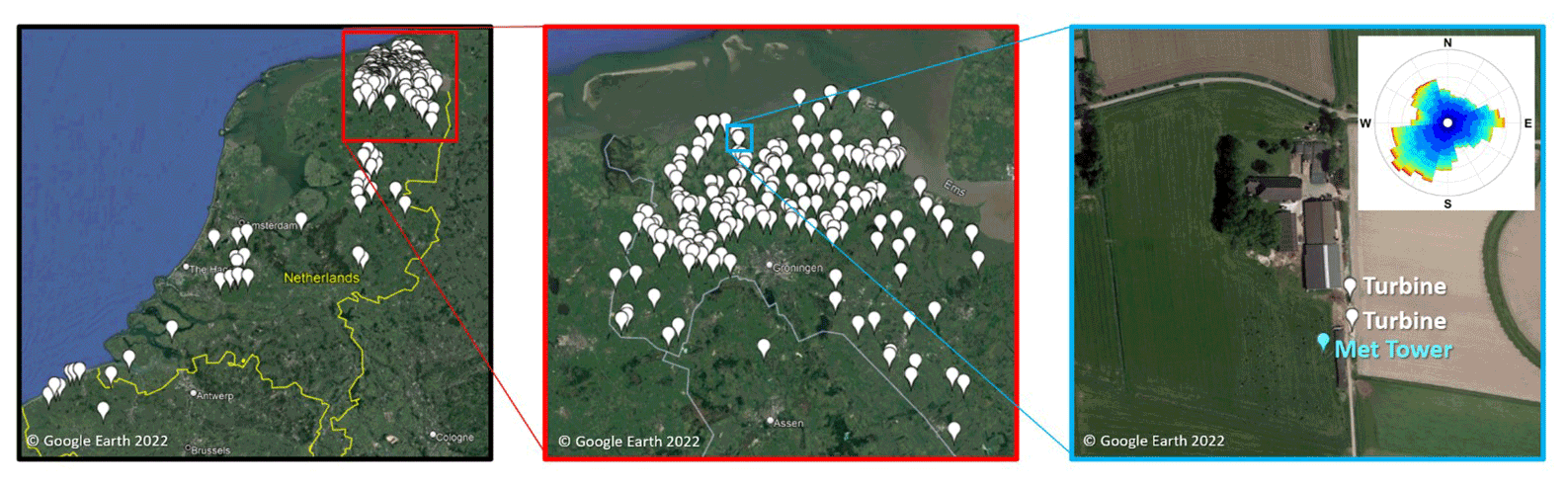
Figure 1Production data were drawn from more than 300 turbines located in the northern Netherlands. Each turbine has a 15 m hub height and provides power production data hourly. The area of detail includes the majority of turbines which are the focus of our obstacle modelling effort. An example site is given in the bottom right of the figure, showing the placement of two specific validation turbines, the IEC meteorological tower, and wind rose for this location. When the wind direction is north/northwest, these turbines are in the wakes of the buildings and trees on the site while other wind directions are largely free of obstructions.
2.1 Production data from turbines
An extensive dataset of measurements from EAZ Wind, a turbine installer and operator in the northern Netherlands, is used to form a basis for evaluating model performance. Figure 1 shows the locations of these turbines as well as an example site used in this study. Additionally, data from one meteorological tower installed for International Electrotechnical Commission (IEC) validation is used. For this tower, wind speed and direction are determined with a calibrated, tower-mounted anemometer. For each turbine, power production data sampled hourly is used to approximate wind speed using a manufacturer provided power curve. All turbines used in this study are EAZ-Twelve with a standardized hub height of 15 m.
When converting power to assumed wind speed, it is not possible to differentiate approximate wind speed for those times when the power production is zero, when the turbine may be curtailed by the grid or offline for maintenance. It is also not possible to differentiate between higher wind speeds when the turbine is operating at rated power. For the remaining cases where the power generation is between 0 and 11 kW, the power curve is invertible, allowing a simple computation of wind speed through interpolation. Those turbines nearby the meteorological tower show good agreement between the anemometer measured wind speeds and those inferred from power generation (RMSE: 0.98 m s−1; MAE: 0.63 m s−1; Mean Bias: −0.15 m s−1). Some of the residual differences between the anemometer and the inferred speeds from power generation are likely due to different wake impacts as the turbines are closer to and more in line with obstacles relative to the dominant wind flow directions compared with the tower.
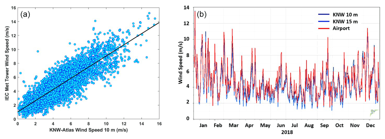
Figure 2Panels (a) and (b) show the approximate accuracy of the KNW-Atlas reanalysis data in the study region. Panel (a) compares reanalysis data at 10 m (no vertical interpolation) with those data collected from the IEC meteorological tower. A small negative bias (−0.12 m s−1) is observed with an R2 of 0.75. Panel (b) compares the KNW reanalysis data product to data from the Amsterdam Schiphol Airport in 2018 using the nearest KNW site (14 km distant).
2.2 Reanalysis mesoscale atmospheric data
Mesoscale reanalysis data from the KNW-Atlas dataset is used as inflow to the models studied. This dataset utilizes the ERA5-Interim as its underlying model (Wijnant et al., 2015). Associated validation studies found that KNW-Atlas overestimates the 10 m winds by 0.3–0.4 m s−1 using satellite-derived offshore winds for most of the North Sea and underestimates the 10 m winds by 0.1–0.3 m s−1 near the Dutch coastline (Stepek et al., 2015). In this dataset, observations from one onshore met tower were used to correct the entire product. Due to the limited prior assessment of onshore accuracy, an independent assessment was performed for the present study. Figure 2 shows the results of this validation, demonstrating agreement with IEC met tower and nearby airport measurements, further confirming the limited prior validation results from Stepek et al. (2015).
In order to map the KNW-Atlas data to the location of each turbine for the purpose of validation, best practices for vertical and spatial interpolation at 40 m hub heights were utilized from prior work by this team (Duplyakin et al., 2021). Specifically, a comparison was made between the inverse distance weighting (with 16 interpolation points) strategy for spatial interpolation and the linear interpolation strategy for vertical interpolation. According to recent work, this combination produced wind estimates with the lowest validation errors, characterized by the mean absolute error estimates obtained for 63 validation sites in the USA (154 site-height combinations). Despite their relative efficacy in the USA, a simpler method utilizing nearest-neighbour spatial interpolation and a log law spatial interpolation was slightly better performing in the area of study; hence, that approach is used here.
An evaluation was performed between two techniques for additional region-level bias correction (BC) of the reanalysis data. BC technique 1 (BC1; turbine data) utilizes wind speed data from each turbine, converted from power as discussed above to fit a multiple linear regression utilizing hour of the day, month of the year, wind direction, and reanalysis wind speed as predictor variables. To prevent underfitting due to the dearth of higher wind speeds in this dataset, a constant 13 m s−1 is imputed when the turbine is operating at rated power. BC technique 2 (BC2; met data) utilizes data from the meteorological tower. While these data are more limited in spatial scope, they are higher resolution, providing greater accuracy. The addition of bias correction resulted in a reanalysis data product closer to observations; however, as both methods necessarily include some effects from obstacles, there may be double counting of obstacle impacts when combined with a separate obstacle model.
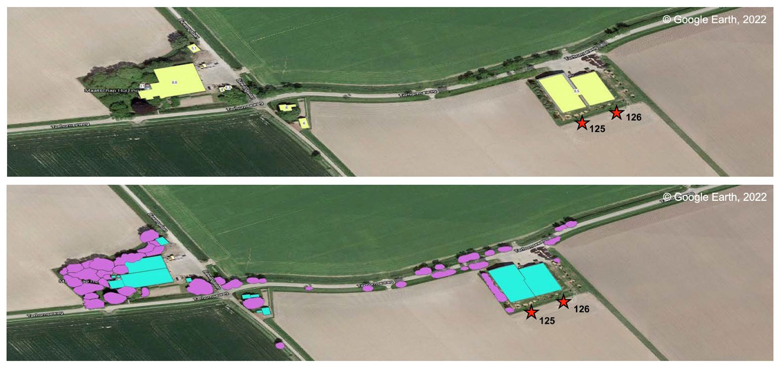
Figure 3Top panel: obstacle annotations for a site with two turbines using data commercially available from 3dBuildings.com. Bottom panel: full annotations using a semi-automated annotation process including both buildings and vegetation, enriched with lidar data.
2.3 Obstacle data
To support obstacle assessment, a standardized method for mapping obstacles was developed. The process begins with information from 3DBuildings (2021), which provides a high-resolution building dataset at the inexpensive average rate of approximately USD 0.06 km−2 and/or USD 0.07 per building for the selected area in northern Netherlands. Similar data can be obtained for other areas in the world; however, the rates are likely to be different as they are directly tied to the level of urbanization in each area of interest. Figure 3a provides an example of the annotations available commercially, which correctly identifies building obstacles. In cases where the commercially available data may be incomplete, and to account for vegetation, which is not included in the commercially available data, a new semi-automated process has been developed using publicly available lidar data from the AHN3 lidar digital surface model (DSM). To simplify annotation, the DSM layer for the 1 × 1 km square encompassing a given turbine is extracted. The DBSCAN clustering technique is used with a convex hull mapping algorithm to determine preliminary obstacle polygons (Schubert et al., 2017). The next step is to manually correct the obstacles and use a visible satellite layer in the QGIS software to modify the polygons around buildings and trees separately. Once the polygons are extracted, it is possible to compute the heights of the obstacles by masking the underlying DSM data with the annotated obstacles and calculate the mean height for each. Figure 3b shows data for the same site with these additions and corrections.
At the end of this process, each building or vegetation obstacle becomes an entry in a geospatial data frame with height estimates accompanying the two- dimensional polygons that represent obstacle shapes. Layers of this data frame can be selected for analysis and visualization of buildings only, vegetation only, or the combination of the two obstacle types. Across the full set of validation sites, filtering out null height obstacles, and considering obstacles with heights greater than 1 m, 257 buildings and 1353 trees/vegetation polygons were located. Building heights range from 1 to 12 m while vegetation heights range from 1 to 15 m.
Table 2 provides a high-level description of the models studied here, each of which is discussed in the following subsections.

3.1 Classic models
The Perera model was developed in 1981 using wind tunnel measurements (Perera, 1981). It provides a closed form equation for the velocity deficit behind a thin (in streamwise direction), infinite-length obstacle of arbitrary porosity, similar to a fence or hedgerow. This model was designed for a scenario where the wind was perpendicular to the length of the obstacle. Despite its apparent limited applicability to other situations, it has found broad applications in commercial tools and remains well known in the small wind community (Poudel et al., 2019). Besides the classic Perera model, various extensions exist including the SHELTER model proposed as part of the WaSP toolkit (Astroup and Larsen, 1999), which allows for limiting the obstacle length to better model buildings and other finite-length shapes. For this study, implementation of these models following the descriptions in the literature was performed. The finite-length version of Perera is referred to here as Perera+.
One significant limitation of both models in their usage for wind turbine siting is that they do not provide reasonable values for obstacles nearer than 5⋅h (or 7⋅h per the original Perera paper), where h is the obstacle height. Figure 4 shows this visually by plotting the velocity deficit factor for different obstacle heights and measurement distances. The triangular region at left of this figure is the area for which Perera should conservatively abstain from making an estimate (locations closer than 5⋅h). Since these nearby locations may incur the largest impact in terms of wake and turbulence on neighbouring turbines, there is significant concern that for DW siting and resource assessment applications the Perera method may underestimate obstacle impacts. Nevertheless, due to their popularity, these models are included as a baseline upon which to compare subsequent models.
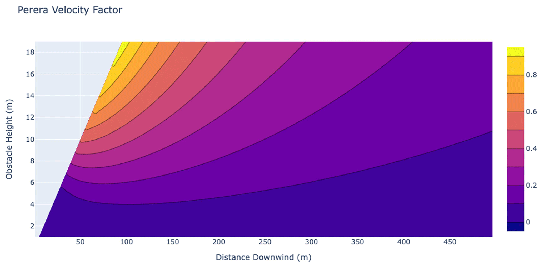
Figure 4Velocity deficit factor prescribed by the Perera model for different combinations of obstacle heights and distances downwind. The missing data in the triangular section at left are those points within 5 h where the model cannot make an accurate estimate.
3.2 ANL and ANL–ML models
Several low-order models (LOM) that are designed to update the Perera model were developed to support this study. An extensive dataset from RANS simulations for the prediction of the flow structure at the wake of buildings (Fytanidis et al., 2021a) were used to train the physics-informed, analytical data-driven model and the solely machine learning based model, referred to herein as ANL and ANL–ML respectively. Specifically, the high-order spectral-element based solver NEK5000 (Fischer et al., 2008) was used to solve three-dimensional turbulent flow equations assuming incompressible flow using realistic boundary conditions to mimic characteristics of real turbulent atmospheric boundary layer flows. The k–τ turbulence closure (Speziale et al., 1992) in combination with the Boussinesq approximation were used for the estimation of Reynolds stresses. The accuracy of the numerical results was evaluated against wind tunnel observations and against results from another numerical model (Fytanidis et al., 2021a, b, using data from Snyder and Lawson, 1994). A grid convergence study was carried out by increasing the polynomial order of the applied computational grids which demonstrated that the produced results are grid independent (Fytanidis et al., 2021a). Additionally, the results of the applied k–τ closure were compared against results produced using the standard k–ε closure and the finite volume solver OpenFOAM. This comparison showed good comparison between the results from the two methods and wind tunnel observations. Finally, no significant difference was observed between the NEK5000 and OpenFOAM results (Fytanidis et al., 2021a, b).
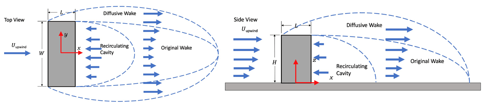
Figure 6The regions where the two wake algorithms, diffusive wake and recirculating cavity, are applied downwind of the building in the QUIC model.
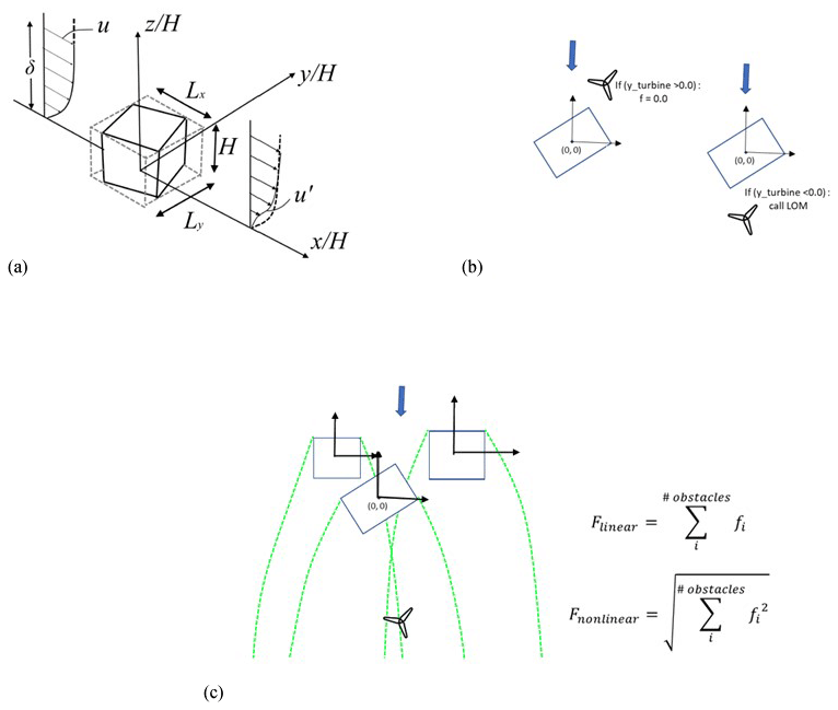
The validated NEK5000 computational results were then used as a training dataset for the evaluation of parameters in a physics-informed, data-driven model (Fytanidis et al., 2021b) that takes into consideration different angles of attack and the effect of different building aspect ratios for the prediction of wake characteristics. Specifically, the dimensions of the enclosing cuboid (Fig. 5a) aligned with the direction of the incoming velocity were used as input parameters for the training of the coefficient for the physics-informed ANL model. The developed model is a new, generalized version able to predict the wake characteristics under various angles of attack and building aspect ratios. Additionally, a correction factor for the prediction of the acceleration due to the formation of a horseshoe vortex around the building was developed (Fytanidis et al., 2021b). The low-order model parameters for various angles of attack and building aspect ratios were estimated using the surrogate model technique combined with the machine learning based algorithms included in the open-source package Tensorflow (Abadi et al., 2015). The applied neural network architecture consists of four branches for the main wake model component of the LOM and three branches for the horseshoe correction of the LOM.
The developed model uses a local coordinate system for each obstacle and evaluates the location of the turbine with respect to the centre of the enclosing cuboid (Fig. 5b). When the turbine is located in the wake of an obstacle, the low-order model evaluates the velocity deficit f. If the turbine is located upwind of the building, the velocity deficit equals zero (f=0). Finally, the solutions for each obstacle were superimposed (Fig. 5c) using a linear and a non-linear superposition technique (see more details in Lissaman, 1979; Katic et al., 1986; and Vogel and Willden, 2020).
3.3 LANL/QUIC model
Models developed for decision support related to transport and dispersion of pollution, chemical–biological–radiological agents, and smoke in population centres cannot be served by CFD approaches due to their computational requirements. Thus, fast-response models have existed for three decades (Röckle, 1990) to serve these specialized applications. These tools fill an important gap in dispersion modelling between extremely rapid but overly simplified flat-earth analytical models typically employed by the emergency response community and the high-fidelity but computationally expensive CFD codes. One of these tools is the Quick Urban & Industrial Complex (QUIC) dispersion modelling system, which was designed to compute wind fields in dense built-up urban areas using the diagnostic wind solver QUIC-URB (Brown et al., 2013). For dispersion modelling, these wind fields are then used by the Lagrangian random-walk model QUIC–PLUME to predict transport and dispersion of gas and particle releases in urban areas. Similarly, QUIC–URB or like-minded models (Kaplan and Dinar, 1996; Wang et al., 2005) can provide wind fields for DW applications where small-scale wind energy developers do not have the time, resources, or expertise to employ higher-fidelity CFD modelling tools. QUIC can run on a laptop with one simulation requiring only seconds to minutes and has been demonstrated to predict wind fields (Neophytou et al., 2011) and plume dispersion footprints (Hertwig et al., 2018) that were comparable to CFD modelling results for practical applications, especially considering the much shorter run times.
The QUIC system's empirical diagnostic wind solver, QUIC-URB, is based on the concept developed by Röckle (1990). The 3D mean wind field is initialized using one or more vertical profiles of wind speed and direction that can either be directly measured or are an extrapolation from a single measurement point. The ambient or background velocities are determined in horizontal planes between all of the profile locations using a two-dimensional Barnes-mapping interpolation scheme. The QUIC-URB model then uses empirical parameterizations to modify the initial wind field to account for building effects (Brown et al., 2013) and vegetative canopy drag (Nelson et al., 2009). The original building wake algorithm as detailed in Röckle (1990) and Kaplan and Dinar (1996) divides the wake downwind of a building into two regions: (a) the recirculating cavity where the flow direction is reversed from the ambient flow and (b) the wake region that transitions the flow back to the undisturbed ambient conditions. The original wake region is defined by a quarter ellipsoid that extends directly downwind of the projected cross section of the building in the direction of the wind without extending laterally to the sides of the building or vertically above the building, similarly to the recirculating cavity seen in Fig. 6 (“Original Wake”). The lack of turbulent diffusion results in a model that cannot accurately predict the reduced velocity above the buildings which can still significantly affect the power produced by a wind turbine that is located downwind of buildings.
To support distributed wind applications, a new diffusive-wake model for QUIC was developed that extends both laterally from the sides and vertically above the top of the building (see Fig. 6 “Diffusive Wake”), using machine learning techniques on time-averaged high-fidelity LES. A set of equations and their parameters describing the stream-wise and crosswind components were developed based on comparisons to wind-tunnel data, high-fidelity models, and general understanding of flow characteristics. Parameters for these functions were determined to be themselves functions of meteorological and building geometry related variables such as atmospheric stability, building dimensions, downwind distance, and relative wind angle. The model was trained against time-averaged data from 72 LES simulations provided by Aeris using Joint Outdoor Urban-indoor LES (JOULES) model (Bieringer et al., 2021) depicting different building dimensions, atmospheric stabilities, and wind angles. Several methods of machine learning were used with the data such as data smoothing, non-linear fitting, and genetic programming to calculate parameters for the governing equations. These methods were derived from a suite of Python packages including PyVista (The PyVista Developers, 2021), SciPy Optimize (The SciPy community, 2021), Statsmodels (Perktold et al., 2021), and GPlearn (Stephens, 2021). Using SciPy's Optimize curve fitting function, parameter values were calculated as a function of downwind distance for each of the 72 cases. GPlearn's symbolic regression algorithms were then used on each of the parameters of these 72 cases to generate equations that are functions of atmospheric stability, building dimensions, downwind distance, and wind angle. With these equations and parameters, the new diffusive wake model was implemented as an optional capability in QUIC–URB. The updated QUIC diffusive model could then be run on a subset of EAZ turbines by creating domains using the QUIC Graphical User Interface (QUIC–GUI) and GeoJSON files containing the building data. Note that all of the building object shapes when resolved in QUIC are converted automatically to rectangular shapes since current functionality of the diffusive wake model is limited to rectangular shapes as shown in Fig. 6.
3.4 Data-driven methods
The aforementioned models are able to make predictions of velocity deficits given only the inflow wind speed, direction, and a description of obstacles. However, when prior data are available, as it is for this study area, there is an additional opportunity to take a data-driven approach, replacing or augmenting simulation-derived and wind-tunnel empirical models like those discussed above with statistical or machine learning models fitted to data from the specific site of interest. It is this observation that motivates the development and validation of an entirely data-driven approach to resource estimation. To this end, observed production data from 307 turbines were utilized to train predictive models that are evaluated on the 20 remaining turbines.
Featurization of the obstacles is the first concern in augmenting the available measurement data so that models can “learn” the impact of obstacles on power generation or wind speed. To strike a balance between computational complexity and detail, the featurization method shown in Fig. 7 was developed. For each turbine, and each of 36 points along the azimuth, all buildings that fall along a 1 km ray are used. For the buildings or obstacles along this path, the number of obstacles (n), the maximum height among obstacles (maxh), the distance to the nearest obstacle (mind), the total cross-sectional distance where there are obstacles (toti), and the distance to the maximum height obstacle (maxhd) are used. Future work may consider deep neural network architectures such as convolutional neural networks (CNNs) that do not require explicit featurization.
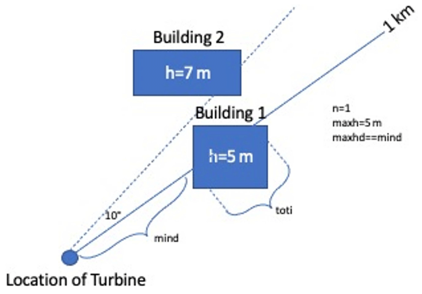
Figure 7An example of featurization in which only one building intersects the 1 km ray at the present angle, so n=1 and maxhd=mind, while maxh=5 (the height of the intersecting building), mind is the distance to the leeward face, and toti is the total length of the intersection in metres.
To choose an effective modelling approach, three different models are evaluated using these same features: (1) multiple linear regression (MLR) fitted by ordinary least squares (OLS), (2) random forest (RF) ensemble, and (3) support vector regression (SVR) with a polynomial kernel. These models were chosen because they are well known and widely available while providing a range of complexity and modelling approaches. Fitting and hyperparameter tuning is performed with the R statistical computing environment (R Core Team, 2021) and caret package (Kuhn, 2021). SVR may be an appropriate technique for modelling non-linear relationships given its polynomial kernel, RF may be most suitable for threshold-based modelling given its underlying tree-based construction, and MLR is useful for providing baseline and easily interpretable results. All models were fitted with and without obstacle features to establish a baseline performance and to predict power generation (directly) and wind speed (indirectly). Due to the computational complexity of fitting the entire dataset and risk in overfitting, 20 000 randomly selected data points are used to fit and tune models, stratified by turbine location and wind direction sector. Experiments using a larger random sample (e.g. 50 000 points) show a small improvement in model performance (∼1 %). Fitted performance and variable importance for the three models are provided in Table 3. The RF approach is able to model the training data most harmoniously, while the MLR approach performs admirably given its simplicity. In practice the improvement associated with adding obstacle features is very small (1 %).
Table 3Variable importance and performance metrics for fitted models. Results for wind speed (m s−1) are given. Results from models predicting power generation are similar. Bold values show the best performing result.

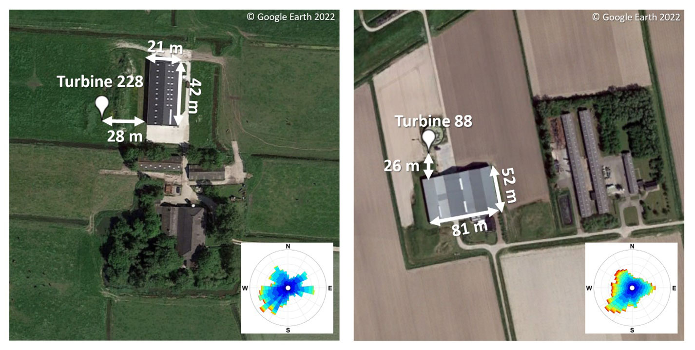
Figure 8Example validation sites (228 and 88) showing a typical turbine location as well as the location of obstacles relative to the turbine.
3.5 Experimental design
To evaluate the models described in the three previous subsections, 20 turbines are held out as a validation set as well as the data from the IEC met tower. The validation set of 20 turbines were chosen from the larger set of 327 because they have significant obstacles in some inflow directions while also representing the geographic diversity and siting complexity in the dataset. Due to the manual nature of some aspects of modelling (in particular, for the QUIC model), and practical feasibility of ensuring accuracy of obstacle descriptions, it was not practical to calculate results for all sites. Hence, it is assumed that this subset of 20 is representative of the larger set. Figure 8 shows two example sites and provides a visual representation of the selection criteria.
Standard error metrics including root mean square error (RMSE), mean absolute error (MAE) and mean bias, for each model and each site are calculated. RMSE is defined as the square root of the mean of the squared differences between observed and predicted wind speeds. MAE is defined as the mean of the absolute value of differences between observed and predicted wind speeds. Mean bias is defined as the mean of these same differences and hence is negative in the case of a systematically negative bias (i.e. underprediction). Besides these metrics, an application-specific measure of error is also calculated: relative error in annual energy production. This metric is computed as follows:
-
Hour–month–sector (HMS) matrix: calculate the average wind speed for each combination of 10∘ wind direction, hour, and month using model predictions.
-
Annualized energy production (AEP): calculate the annual production estimate (MWh) for this site using historical reanalysis data and the HMS matrix as a lookup table.
-
Relative error in AEP estimate: compute the percentage difference between the AEP estimate and the true production of the turbine during the period of study.
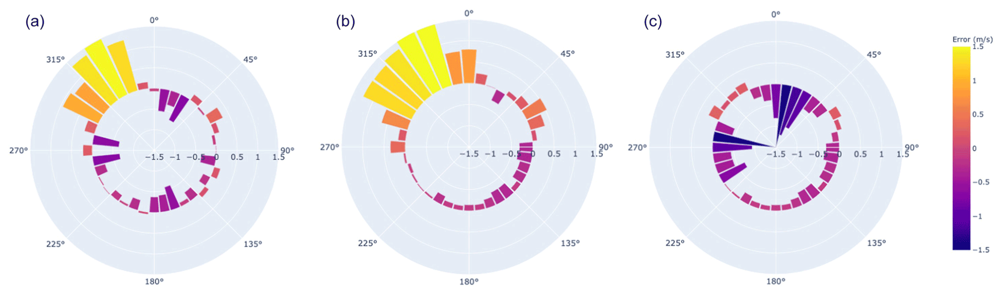
Figure 9Average error in m s−1 for IEC site grouped by wind speed direction (10∘ sectors) for (a) LANL/QUIC, (b) KNW-Atlas reanalysis, and (c) ANL non-linear. Positive errors (lighter colours) suggest an overestimate of the wind resource relative to observed data, whereas negative errors (darker colours) indicate the opposite. The scale of errors for each plot is given on the radial access.
To understand the practical performance of models relative to the conditions in which they are applied, each model is evaluated with basic obstacle descriptions and unaltered inflow data as well as two other scenarios: (1) with prior bias correction applied to the inflow and (2) with enhanced obstacle data including vegetation.
The results are subdivided below into those that utilize the 8 months of meteorological tower data and those that utilize the validation set of 20 turbines. Due to the inherent strengths and limitations of each performance assessment, these should be taken together to draw a conclusion about practical performance.
4.1 Results for IEC tower
Combined results are provided for the IEC tower site (pictured in Fig. 1) in Table 4. While this is only one site, the data are of high quality for the 8-month study period. The KNW-Atlas reanalysis data product significantly overestimates the wind speed at this site, resulting in an approximately 13 % overestimation in annual production that might be achieved (mean bias 0.25 m s−1). It is assumed that this overestimate is due to the need for obstacle velocity deficit correction. Indeed, when applied, each obstacle correction model reduces the degree of overestimation. However, some models cause too great of an adjustment and skew the results towards the negative. The best-performing model overall is the LANL/QUIC model, achieving <1 % relative error (positive bias) in production across the 8 months, followed by Perera (6.4 % relative error, positive bias). The best-performing model with a negative bias is the data-fitted bias correction model (no obstacles considered) resulting in an average relative error of −8.8 %. The data-fitted models are likely less performant here because they were fitted with turbine data from other EAZ turbines, and hence are optimized to predict turbine performance rather than anemometer measurements.
Table 4Results comparison for IEC Met Tower. Bold values show the results of best performance.

n/a: not applicable.
Figure 9 compares the error process for both the inflow reanalysis data and the QUIC/LANL and ANL methods using a polar plot. As this site has the bulk of obstacles located to the NNW, it is reasonable to expect the error in this direction, whereas the other dominant modalities in wind direction (W and SE) appear unobstructed. The plots show that the QUIC/LANL model makes only modest adjustments to the positive bias in the NNW direction and most significantly addresses overestimates in less-dominant wind flow directions (N and NW). By comparison, the ANL model does better to address the overestimate of wind speeds in the direction of obstacles (NNW) but also exaggerates these effects in some directions (W and NNE). These results suggest there is significant sensitivity in the choice of obstacle model: in some cases the choice may cause more harm than good in environments where the underlying reanalysis data have relatively low bias, the terrain is simple, and turbines can be located to minimize interference from obstacles in the dominant direction of wind flow.
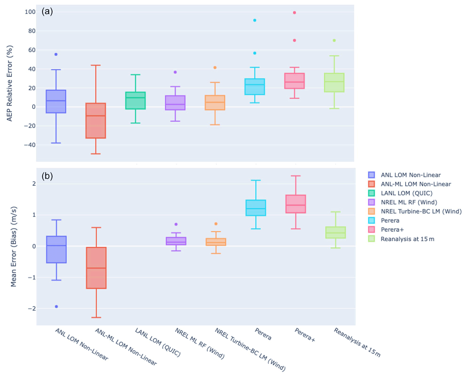
Figure 10Box and whisker plots showing performance (median, IQR, 90th percentiles, and outliers) for the models studied for annual production estimate relative error (a) and mean pointwise wind speed bias (b).
4.2 Results for turbine validation set
In the next phase of analysis, similar metrics are calculated for the larger dataset of 20 selected validation turbine locations. Table 5 and Fig. 10 provide the combined results. The most performant models across a variety of sites are the data-driven models. This stands to reason since these models were able to benefit from the rich multiyear dataset of production from turbines in this same environment. Interestingly, the addition of obstacle features adds only a very small (∼1 %) improvement to the overall accuracy of this data-driven method, suggesting that local bias correction without obstacle models may be sufficient in regions with similar topography and well-sited turbines with few large obstacles. Among those models that operate without a priori information, the LANL/QUIC and ANL non-linear models both perform well with an 8 % and 12 % average error respectively, though the LANL/QUIC model has a smaller spread in its error distribution. The Perera model makes very conservative adjustments to the inflow reanalysis data. These results again suggest a high degree of sensitivity in model selection with some models overestimating or underestimating the annual production by as much as 40 % or 60 % for individual turbines. When existing production data are available, the best approach for these sites appears to be one driven by prior measurements, achieving 3 %–5 % less mean error.
Table 5Results comparison for validation sites (averages). Bold values show the best performing result for each metric.
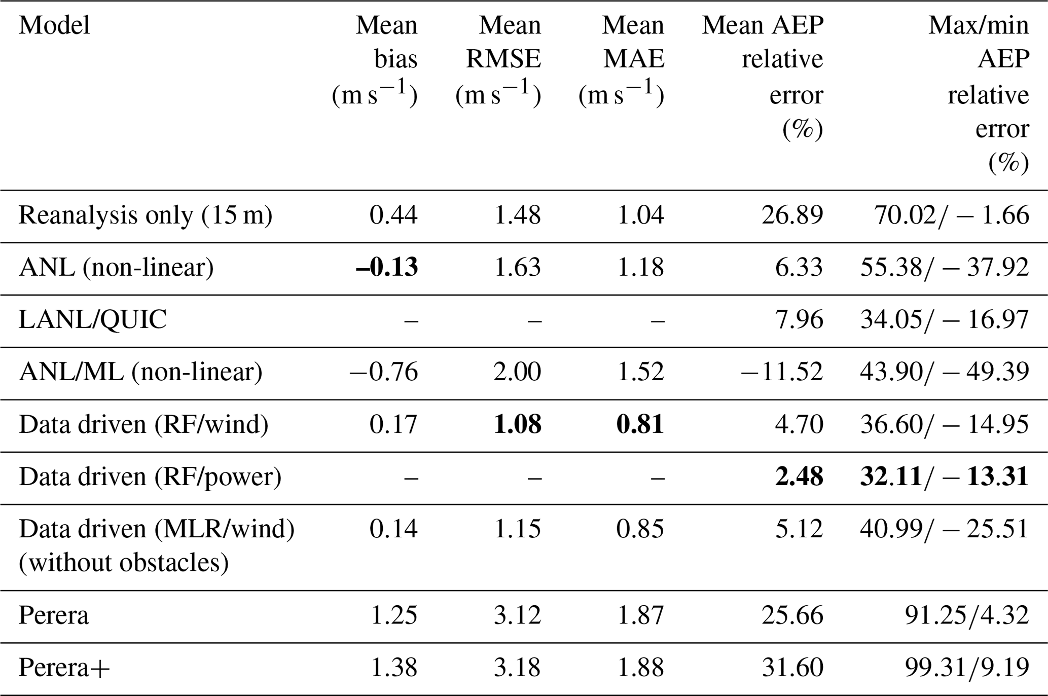
Figure 11Box and whisker plots showing performance (median, IQR, 90th percentiles, and outliers) for the models studied, both with and without local bias correction applied prior to obstacle impact assessment. The six boxes on the left of the plot correspond to the models with and without bias correction, while the three on the right are the inflow data and bias corrected data without obstacle assessment.
Figure 12Box and whisker plots showing performance (median, IQR, 90th percentiles, and outliers) for the models studied, both with and without additional obstacles. The eight boxes on the left of the plot correspond to the models with and without additional obstacles, while the one on the right shows inflow without obstacle assessment.
4.3 Bias correction before obstacle correction
Being that the data-driven methods perform very well in our analysis, and even without obstacle features, one potential approach would be to combine a data-fitted regional/site level bias correction with a subsequent obstacle model (i.e. Perera, LANL QUIC, or ANL LOM). In this scenario, the obstacle models would begin with velocity estimates that are closer to observation, perhaps reducing their error but also with the risk of double-counting the effect of obstacles. To understand the practical efficacy of this hybrid approach, the performance of each model is assessed with and without prior bias correction. Figure 11 shows the result of this experiment. For all models, the addition of prior bias correction significantly reduces the wind speed estimates, causing a negative mean bias and thereby underestimating the performance of the turbines in most cases. The Perera model does perform better with bias correction; however, this is likely due to the degree to which the Perera model overestimates the wind velocity rather than as a result of a uniquely positive interaction between these two models. On the right-hand side of this plot, we can see the performance for bias correction alone, without obstacle assessment, which tends to perform better (error much closer to zero) than all models except Perera as noted above. Based on these results, the derived recommendation is that either local (data-fitted) bias correction be applied when data are available or obstacle correction, when data are not available, but not both. All models still outperform reanalysis data alone.
4.4 Quality of obstacle data
As a final consideration in the configuration, all models were run for all selected sites using both the building-only obstacle data available commercially from 3DBuildings.com and with those using our semi-automated annotation method, utilizing lidar data and manual inspection to add additional buildings and vegetation. Notably not all models are designed to model vegetation, so for those models that do not explicitly include it (ANL LOM and Perera), vegetation is treated as if it is a collection of solid obstacles of the same rectilinear sizes and shapes.
Figure 12 shows the result of this experiment. In nearly all cases, adding additional obstacles (whether additional buildings or vegetation) results in generally lower wind speed predictions at the turbine locations. The ANL models overestimate the effect of obstacles in this case, causing an overall negative bias for most sites and thereby underestimating the performance of the turbine. This is a net improvement as the mean error for the simple obstacles is 6 % and the performance with added obstacles is −6 %. Generally, a small negative error is likely preferable to a positive error for the purpose of performance estimation in siting. Overall, the error spread stays high for this model, however, and at some sites the error is greater than 20 %. The diffusive wake LANL model achieves similar performance with the added obstacles (8 %–8.5 % mean error), likely due to a more sophisticated multi-obstacle method and functions designed for the inclusion of vegetation. The Perera model performs somewhat better with more obstacles but still overestimates wind speeds. The data-fitted NREL model performs similarly, having nearly identical mean error characteristics (2.5 %–2.8 %) and spread.
These results show the sensitivity of the models studied to the quality of obstacle input data. While generally the results are similar with higher-fidelity obstacle data, there are also cases where the added obstacles (or vegetation) may cause a model to underestimate wind speeds significantly (i.e. overestimate the impact of obstacles). The best-performing models also perform slightly worse in the mean (and slightly better in the median). When it is possible to collect observational data prior to deploying turbines, or when data from previously deployed turbines are available, it is likely advisable to conduct a data-informed model selection and calibration, thereby determining the best model for a given region and the necessary detail in obstacle data to maximize practical performance. Also, in areas with significant vegetation, it may be most appropriate to consider whether modelling vegetation is necessary.
This study provides a first of its kind analysis comparing a wide variety of obstacle modelling approaches in the practical setting of distributed wind resource assessment and small wind turbine siting. Mesoscale reanalysis datasets may not adequately consider local topography and obstacles resulting in a significant overestimate in wind speed and performance at typical sites. When possible, data-driven methods fitted to production actuals or measurements from mast-mounted anemometers provide the best opportunity to bias correct the wind resource from mesoscale models, providing the greatest relative benefit. In the absence of site-specific measurements, lower-order obstacle models improve estimates at some sites (by as much as 10 %–15 % in annual production estimates), but the resulting accuracy may be sensitively dependent on the choice of model, the quality of the inflow data, and the fidelity of obstacle descriptions. Classic models such as Perera underestimate the impact of obstacles, while in certain circumstances the newer models may overestimate the impact of obstacles, resulting in negative bias. This tendency is compounded when combining multiple models (e.g. bias correction and obstacle models) or using higher-fidelity obstacle metadata that includes vegetation. The LANL/QUIC model performs best among the lower-order models studied; however, its computational cost is slightly higher than that of the other models studied and controls on export may hinder broad international adoption.
This study does have several limitations that must be recognized in interpreting the findings:
-
The northern Netherlands is an agricultural region, at sea level, with relatively undisturbed inflow wind and very low terrain complexity. To the extent possible, turbine locations have also been chosen to minimize impact from obstacles. Hence, our results are likely limited to those in similar environments and should not be applied in widely different settings. Future work will continue these studies in additional settings such as moderately built environments in the central USA, as well as environments with more terrain complexity such as the mountainous western regions of the USA.
-
Though anemometer measurements are utilized for the IEC site, the bulk of the dataset is derived from turbine production data which has inherent limits in both accuracy and the ability to infer wind speed ex post facto. Measurements from production wind turbines necessarily limit the impact of obstacles because siting decisions have been made to avoid them. Notably, however, broad agreement exists in the conclusions from both anemometer and production-inferred datasets. Nevertheless, these results should be reconfirmed when additional meteorological data are available.
-
A range of models have been studied, from those just introduced to those introduced more than 30 years ago. The most recent models are still being actively developed and improved, and it is entirely possible that future versions may perform better or differently.
In summary, based on the conclusions of this study, small wind operators should take care when accounting for obstacles, and whenever possible the greatest benefit is likely to be realized through measurement campaigns and careful use of existing mesoscale data products, ideally coupled with bias correction. Small wind operators may wish to consult multiple data products and techniques in their analysis in order to determine a range of possible results instead of just one. When a priori obstacle impacts are needed, without pre-existing data, modern lower-order models are likely to reduce error as compared with classic models such as Perera. As compared with data-fitted models, analytical models may find additional value in micro-siting applications where the exact velocity deficit due to obstacles is not needed, but rather the shape and extent of their impacts. Future work will extend and improve upon these results by considering additional environments and applications.
Software for the developed models is currently being prepared for release through our project website https://doi.org/10.11578/dc.20200925.11 (Phillips et al., 2020) and API (https://dw-tap.nrel.gov/; Duplyakin et al., 2022).
Data used in this study are either already available publicly (e.g. KNW-Atlas reanalysis data, AHN3 lidar data) or proprietary (e.g. EAZ turbine production data). We do not expect to release additional supporting data with this publication.
Concept, manuscript preparation, software development, and execution were performed by CP. Validation methodology was developed by LS. Models were developed by CP, PC, DF, MN, and ND. Obstacle mapping methodology was developed by SZ and DD. Interpolation methodology and evaluation was developed by DD. All authors contributed to manuscript edits, technical review, and interpretation of results.
The contact author has declared that neither they nor their co-authors have any competing interests.
Publisher's note: Copernicus Publications remains neutral with regard to jurisdictional claims in published maps and institutional affiliations.
The team also gratefully acknowledge the computing resources provided on Bebop, a high-performance computing cluster operated by the Laboratory Computing Resource Center at Argonne National Laboratory, and the computing resources provided on Eagle, a high-performance computing cluster operated by the National Renewable Energy Laboratory.
This work is supported by the Department of Energy's (DOE) Energy Efficiency and Renewable Energy (EERE) Wind Energy Technologies Office (WETO) under contract DE-AC02-06CH11357.
This paper was edited by Alessandro Bianchini and reviewed by three anonymous referees.
Abadi, M., Agarwal, A., Barham, P., Brevdo, E., Chen, Z., Citro, C., Corrado, G. S., Dean, A. J., Devin, M. ,Ghemawat, S., Goodfellow, I., Harp, A., Irving, G., Isard, M., Jozefowicz, R., and Zheng, X.: Tensorflow: Large-scale machine learning on heterogeneous distributed systems, arXiv preprint: arXiv:1603.04467, 2015.
Astroup, P. and Larsen, S. E.: WAsP Engineering Flow Model for Wind over Land and Sea, Riso National Laboratory, Roskilde, Denmark, ISBN 87-550-2529-3, August 1999.
Bieringer, P. E., Piña, A. J., Lorenzetti, D. M., Jonker, H. J. J., Sohn, M. D., Annunziao, A. J., and Fry, R. N.: A graphics processing unit (GPU) approach to large eddy simulation (LES) for transport and contaminant dispersion, Atmosphere, 12, 890, https://doi.org/10.3390/atmos12070890, 2021.
Brown, M., Gowardhan, A., Nelson, M., Williams, M., and Pardyjak, E.: QUIC transport and dispersion modelling of two releases from the joint urban 2003 field experiment, Int. J. Environ. Pollut., 52, 263–287, 2013.
Bruse, M. and Fleer, H.: Simulating surface–plant–air interactions inside urban environment with a three dimensional numerical model, Environ. Model. Softw., 13, 373–384, https://doi.org/10.1016/S1364-8152(98)00042-5, 1998.
Castro, I. P., Xie, Z. T., Fuka, V., Robins, A. G., Carpentieri, M., Hayden, P., Hertwig, D., and Coceal, O.: Measurements and computations of flow in an urban street system, Bound.-Lay. Meteorol., 162, 207–230, 2017.
Counihan, J. J. C. R., Hunt, J. C. R., and Jackson, P. S.: Wakes behind two-dimensional surface obstacles in turbulent boundary layers, J. Fluid Mech., 64, 529–564, 1974.
Drew, D. R., Barlow, J. F., Cockerill, T. T., and Vahdati, M. M.: The importance of accurate wind resource assessment for evaluating the economic viability of small wind turbines, Renew. Energy, 77, 493–500, https://doi.org/10.1016/j.renene.2014.12.032, 2015.
Duplyakin, D., Zisman, S., Phillips, C., and Tinnesand, H.: Bias Characterization, Vertical Interpolation, and Horizontal Interpolation for Distributed Wind Siting Using Mesoscale Wind Resource Estimates, NREL/TP-2C00-78412, NREL – National Renewable Energy Laboratory, Golden, CO, USA, https://doi.org/10.2172/1760659, 2021.
Duplyakin, D., Zisman, S., Phillips, C., and Tinnesand, H.: DW-TAP API, NREL [code], https://dw-tap.nrel.gov, last access: 24 May 2022.
Fields, J., Tinnesand, H., and Baring-Gould, I.: Distributed Wind Resource Assessment: State of the Industry, NREL/TP-5000-66419, NREL – National Renewable Energy Laboratory, Golden, CO, USA, https://doi.org/10.2172/1257326, 2016.
Fischer, Paul, Lottes, J., Pointer, D., and Siegel, A.: Petascale algorithms for reactor hydrodynamics, J. Phys.: Conf. Ser., 125, 012076, https://doi.org/10.1088/1742-6596/125/1/012076, 2008.
Fytanidis, D. K., Tombloulides, A. G., Balakrishnan, R., Kotamarthi, R., and Fischer, P.: Reynolds Average Navier-Stokes simulations of atmospheric boundary layer flows around building-like obstacles using NEK5000, in: 13th International ERCOFTAC symposium on engineering, turbulence, modelling and measurements, ETMM13, 15–17 September 2021, Rhodes, Greece, https://cdn.knmi.nl/knmi/pdf/bibliotheek/knmipubTR/TR352.pdf (last access: 24 May 2022), 2021a.
Fytanidis, D. K., Maulik, R., Balakrishnan, R., and Kotamarthi, R.: A physics-informed data-driven low order model for the wind velocity deficit at the wake of isolated buildings, Report ANL-21/24, Argonne National Laboratory, https://doi.org/10.2172/1782670, 2021b.
Gowardhan, A. A., Pardyjak, E. R., Senocak, I., and Brown, M. J.: A CFD-based wind solver for an urban fast response transport and dispersion model, Environ. Fluid Mech., 11, 439–464, 2011.
Hertwig, D., Soulhac, L., Fuka, V., Auerswald, T., Carpentieri, M., Hayden, P., Robins, A., Xie, Z.-T., and Coceal, O.: Evaluation of fast atmospheric dispersion models in a regular street network, Environ. Fluid Mech., 18, 1007–1044, https://doi.org/10.1007/s10652-018-9587-7, 2018.
Hussein, H. J. and Martinuzzi, R. J.: Energy balance for turbulent flow around a surface mounted cube placed in a channel, Phys. Fluids, 8, 764–780, 1996.
Kaplan, H. and Dinar, N.: A Lagrangian dispersion model for calculating concentration distribution within a built-up domain, Atmos. Environ., 30, 4197–4207, 1996.
Katic, I., Højstrup, J., and Jensen, N. O.: A simple model for cluster efficiency, in: Vol. 1, Proceedings of the European Wind Energy Conference, Rome, Italy, 407–410, https://backend.orbit.dtu.dk/ws/portalfiles/portal/106427419/A_Simple_Model_for_Cluster_Efficiency_EWEC_86_.pdf (last access: 24 May 2022), 1986.
Kothari, K. M., Peterka, J. A., and Meroney R. N.: Stably stratified building wakes, Colorado State University, https://www.osti.gov/biblio/5595682 (last access: 24 May 2022), 1980.
Krajnović, S., Müller, D., and Davidson, L.: Comparison of two one-equation subgrid models in recirculating flows, in: Direct and large-eddy simulation III, Springer, Dordrecht, 63–74, https://doi.org/10.1007/978-94-015-9285-7_6, 1999.
Kuhn, M.: caret: Classification and Regression Training, R package version 6.0-88, https://CRAN.R-project.org/package=caret, last access: 29 December 2021.
Lakehal, D. and Rodi, W.: Calculation of the flow past a surface-mounted cube with two-layer turbulence models, J. Wind Eng. Indust. Aerodynam., 67, 65–78, 1997.
Lissaman P.: Energy effectiveness of arbitrary arrays of wind turbines, J. Energy, 3, 323–328, 1979.
Martinuzzi, R. and Tropea, C.: The flow around surface-mounted, prismatic obstacles placed in a fully developed channel flow (data bank contribution), J. Fluids Eng., 115, 85–92, https://doi.org/10.1115/1.2910118, 1993.
Nelson, M. A., Williams, M. D., Zajic, D., Pardyjak, E. R., and Brown, M. J.: Evaluation of an urban vegetative canopy scheme and impact on plume dispersion, in: 8th Symposium on the Urban Environment, American Meteorological Society, Phoenix, Arizona, USA, JP6.4, 2009.
Neophytou, M., Gowardhan, A. and Brown, M.: An inter-comparison of three urban wind models using the Oklahoma City Joint Urban 2003 wind field measurements, Int. J. Wind Eng. Indust. Aerodynam., 99, 357–368, 2011.
Orrell, A. C., Kazimierczuk, K., and Sheridan, L. M.: Distributed Wind Market Report: 2021 Edition, DOE/GO-102021-5620, PNNL – Pacific Northwest National Laboratory, Richland, WA, USA, https://doi.org/10.2172/1817750, 2021.
Perera, M. D. A. E. S.: Shelter Behind Two-Dimensional Solid and Porous Fences, J. Wind Eng. Indust. Aerodynam., 9, 93–104, 1981.
Perktold, J., Seabold, S., and Taylor, J.: LOWESS (Locally Weighted Scatterplot Smoothing), https://www.statsmodels.org/dev/generated/statsmodels.nonparametric.smoothers_lowess.lowess.html, last access: 30 November 2021.
Peterka, J. A., Meroney, R. N., and Kothari, K. M.: Wind flow patterns about buildings, J. Wind Eng. Indust. Aerodynam., 21, 21–38, 1985.
Phillips, C., Duplyakin, D., Zisman, S., and USDOE Office of Energy Efficiency and Renewable Energy: DW TAP Computational Framework [Computer software], DOE [code], https://doi.org/10.11578/dc.20200925.11, 2020.
Poudel, R., Tinnesand, H., and Baring-Gould, I. E.: An Evaluation of Advanced Tools for Distributed Wind Turbine Performance Estimation, J. Phys.: Conf. Ser., 1452, 012017, https://doi.org/10.1088/1742-6596/1452/1/012017, 2019.
R Core Team: R: A language and environment for statistical computing, R Foundation for Statistical Computing, Vienna, Austria, https://www.R-project.org/, last access: 29 December 2021.
Robins, A. G. and Apsley, D. D.: Modelling of building effects in ADMS, http://www.cerc.co.uk/environmental-software/assets/data/doc_techspec/P16_01.pdf, last access: 10 March 2021.
Röckle, R.: Bestimmung der stomungsverhaltnisse im bereich komplexer be bauungsstrukturen, PhD thesis, Vom Fachbereich Machanik, der Technischen Hochshule, Darmstadt, Germany, https://www.worldcat.org/title/bestimmung-der-stromungsverhaltnisse-im-bereich-komplexer (last access: 24 May 2022), 1990.
Schofield, W. H. and Logan, E.: Turbulent shear flow over surface mounted obstacles, J. Fluids Eng., 112, 376–385, https://doi.org/10.1115/1.2909414, 1990.
Schubert, E., Sander, J., Ester, M., Kriegel, H. P., and Xu, X.: DBSCAN revisited, revisited: why and how you should (still) use DBSCAN, ACM Transactions on Database Systems (TODS), 42, 1–21, 2017.
Snyder, W. H. and Lawson R. E.: Wind-tunnel measurements of flow fields in the vicinity of buildings, US Environmental Protection Agency, Washington, DC, EPA/600/A-93/230 (NTIS PB93236594), 1994.
Speziale, C. G., Abid, R., and Anderson, E. C.: Critical evaluation of two-equation models for near-wall turbulence, P. AIAA, 30, 324–331, 1992.
Stepek, M., Savenije, H. W., and Van den Brink, I. L.: Validation of KNW atlas with publicly available mast observations (Phase 3 of KNW project), Technical report, KNMI Technical Report TR352, KNMI, https://cdn.knmi.nl/knmi/pdf/bibliotheek/knmipubTR/TR352.pdf (last access: 24 May 2022), April 2015.
Stephens, T.: Genetic Programming in Python with a scikit-learn inspired API, https://gplearn.readthedocs.io/en/stable/, last access: 29 December 2021.
The PyVista Developers: Surface Smoothing: Smoothing rough edges of a surface mesh, Retrieved from Pyvista: 3D plotting and mesh analysis through a streamlined interface for the Visualization Toolkit (VTK), https://docs.pyvista.org/examples/01-filter/surface-smoothing.html, last access: 29 December 2021.
The SciPy community: scipy.optimize.curve_fit: Use non-linear least squares to fit a function, f, to data, https://docs.scipy.org/doc/scipy/reference/generated/scipy.optimize.curve_fit.html, last access: 29 December 2021.
3DBuildings: 3DBuildings, https://3dbuildings.com/, last access: 29 December 2021.
Tominaga, Y. and Stathopoulos, T.: CFD Simulations of near-field pollutant dispersion in the urban environment: a review of current modelling techniques, Atmos. Environ., 79, 716–730, 2013.
Tominaga, Y. and Stathopoulos, T.: Ten questions concerning modeling of near-field pollutant dispersion in the built environment, Build. Environ., 105, 390–402, 2016.
Vogel, C. R. and Willden, R. H. J.: Investigation of wind turbine wake superposition models using Reynolds-averaged Navier-Stokes simulations, Wind Energy, 23, 593–607, 2020.
Wang, Y., Williamson, C., Garvey, D., Chang, S., and Cogan, J.: Application of a multigrid method to a mass-consistent diagnostic wind model, J. Appl. Meteorol., 44, 1078–1089, https://doi.org/10.1175/JAM2262.1, 2005.
Wijnant, I. L., Marseille, G. J., Stoffelen, A., van den Brink, H. W., and Stepek, A.: Validation of KNW atlas with scatterometer winds (Phase 3 of KNW project), Tech. Rep. TR 353, KNMI, De Bilt, the Netherlands, https://cdn.knmi.nl/knmi/pdf/bibliotheek/knmipubTR/TR353.pdf (last access: 24 May 2022), 2015.
Yakhot, A., Liu, H., and Nikitin, N.: Turbulent flow around a wall-mounted cube: A direct numerical simulation, Int. J. Heat Fluid Flow, 27, 994–1009, 2006a.
Yakhot, A., Anor, T., Liu, H., and Nikition, N.: Direct numerical simulation of turbulent flow around a wall-mounted cube: spatio-temporal evolution of large-scale vortices, J. Fluid Mech., 566, 1–9, 2006b.