
Downloads
Download


This work is licensed under a Creative Commons Attribution 4.0 International License.
Article
Real-Time Sensing and Fault Diagnosis for Transmission Lines
Fatemeh Mohammadi Shakiba 1, Milad Shojaee 1, S. Mohsen Azizi 1,2, and Mengchu Zhou 1,*
1 Department of Electrical and Computer Engineering, New Jersey Institute of Technology, Newark 07102, NJ, USA.
2 The school of Applied Engineering and Technology, New Jersey Institute of Technology, Newark 07102, NJ, USA.
* Correspondence: mengchu.zhou@njit.edu
Received: 12 October 2022
Accepted: 8 November 2022
Published: 22 December 2022
Abstract: Protection of high voltage transmission lines is one of the crucial problems in the power system engineering. Accurate and timely detection and identification of transmission line short circuit faults can considerably improve and simplify their recovery process and hence save the costs associated with the downtime of a power system. Hence, it is essential that a robust and reliable fault diagnosis system completes its operation within an acceptable time window after fault occurrence in the presence of uncertainties and disturbances in the system. The significant costs of mistakenly detected or undetected faults based on the conventional techniques motivate us to present a robust detection and identification system by using the convolutional neural networks. The robustness of this technique is analyzed for the variations of the phase difference between two connected buses, fault resistance, source inductance fluctuations, fault inception angle, local bus voltage fluctuations, and measurement noises. The time delay analysis is also conducted to indicate that the presented technique is able to detect, identify, and estimate the location of faults before tripping relays and circuit breakers disconnect a faulty region.
1. Introduction
Transmission lines (TLs) are one of the most salient parts of a power delivery system. They are exposed to unexpected and severe atmospheric conditions, making them prone to faults [ 1 ]. Therefore, detection, identification, and location estimation methods such as machine learning-based ones are essential for an efficient and timely repair of TL faulty regions and reduction of the excessive costs of triggering circuit breakers when faults are detected mistakenly [ 2 ]. Since tripping relays and circuit breakers become active rapidly, it is crucial that a fault diagnosis system can make use of the limited amount of data received during the interval between the occurrence of a fault and the tripping of relays and circuit breakers.
TL fault identification and estimation techniques are categorized into two major classes based on the number of terminals utilized for sensing and acquiring data: single-terminal and multi-terminal techniques. Each can be further subcategorized depending on the type of data measurement and the algorithms used for data analysis [ 3 ]. The following groups are presented in this categorization:
• Signal processing-based techniques that usually consider three-phase currents as input signals. These techniques can handle the problem of fault detection and prediction of the abnormalities occurring in the system. They include different schemes such as Wavelet transform [ 4 ], Fourier-Taylor transformation [ 5 ], and Power spectral density index [ 6 ].
• Phasor-based methods that take advantage of phasor measurement units [ 7 - 9 ]. In these approaches, the presented techniques are capable of detecting short circuit faults for both balanced and unbalanced systems.
• Machine learning-based methods include neural networks (NNs) [ 10 - 12 ], support vector machines (SVMs) [ 13 ], decision trees [ 14 , 15 ], Summation-Wavelet and Summation-Gaussian extreme learning machines [ 16 ], generalized regression neural networks (GRNNs) [ 13 , 15 , 17 ], feedforward neural networks (FNNs) [ 18 - 22 ], and convolutional neural networks (CNNs) [ 23 - 25 ]. These methods are powerful in identifying abnormal patterns and distinguishing between a faulty system and a healthy system.
• Travelling wave (TW)-based methods [ 26 , 27 ] that are used to detect and localize faults based on the arrival time of the transient waves generated by faults. In addition, this group contains fast and accurate methods that require measurement devices with high sampling rates.
• Other miscellaneous techniques such as fuzzy logic [ 28 , 29 ], vector rotation [ 30 ], phase-locked loop [ 31 ], and transient monitor index [ 32 ].
1.1. Motivation
Some approaches focus on addressing the problem of fault detection using TW-based techniques [32-37]. The advantages of these techniques include their independence from the network topology and resilience to load changes, high grounding resistance and series capacitors. On the other hand, they suffer from being costly, requiring a high sampling rate for capturing the high frequency fault transients, restricted proficiency to differentiate between waves returned from a fault point and the distant end of a TL, and the hardships of detecting the zero-crossing-based faults [38, 39]. Moreover, the performance of TW-based methods is sensitive to high impedance faults and source inductance changes. These variations transmute the transient wave shapes and hence, TW-based methods can barely capture the correct arrival time of the transient waves.
Another pitfall of TW-based methods in the literature is that they have not reported the accuracy of their fault diagnosis system. To put it differently, they have not reported any statistical results to demonstrate the performance of their technique in terms of erroneously detected or undetected faults. There are many disturbances, uncertainties, and noise in the transmission line that could make transient waves similar to the faulty waves and hence lead to mistakenly detected or undetected faults and power outages. According to the reports from the U.S. Department of Energy, the annual cost of power outages for American businesses is estimated to be around $150 Billion [40]. Accordingly, a high level of accuracy in fault detection is demanded in order to reduce the rate of power outages resulting from mistakenly detected or undetected faults. The NN-based technique used in this article makes use of the amplitudes of the fundamental frequency component of the voltage and current signals to avoid dealing with the transient waves generated from faults. Thus, as it will be shown later, the performance of such methods is not adversely affected by the changes in current and voltage transients, and this feature makes the NN-based approaches more effective and economical.
1.2. Literature Review
According to the aforementioned disadvantages of TW-based techniques, multiple studies are performed on fault detection and identification based on artificial intelligence approaches such as NNs, SVMs, neuro-fuzzy networks, etc., and signal processing procedures such as fast Fourier transform (FFT), wavelet transform (WT), etc. In [4], authors use WT for extracting the features and SVM for identifying faulty sections, which is a computationally expensive approach. In [14], authors employ a decision tree regression-based method together with FFT and discrete wavelet transform (DWT) for fault distance estimation, which is a noise sensitive methodology. Reddy et al. in [41] propose an approach based on synchronized current measurements of isolated telemetry units (ITUs) installed on both ends of a TL. In their study, SVMs are utilized to calculate the fault distance using the extracted features, and ANFIS is built to improve the efficiency of their proposed scheme. Their study does not perform the robustness analysis, and their proposed technique's performance is sensitive to noise. Summation-Wavelet extreme learning machine and Summation-Gaussian extreme learning machine are studied in [16] for fault location estimation and identification.
In [10], a novel zone division method using NNs is developed for power system fault detection in which the features are extracted by using an extended Kalman filter. This methodology requires heavy computation, and is therefore not efficient. Koley et al. [42] propose a methodology using a hybrid wavelet transform and FNN model to detect, classify, and locate six-phase TL faults using single-end data. In this scheme, the standard deviation of the approximate coefficients of voltage and current signals are gathered using DWT and fed to the modular FNN for fault identification and location estimation. In [43], a technique based on S-transform and Probabilistic NN is presented that is unable to handle noisy situations very well. An SVM-based technique for fault identification and location estimation problems is investigated in [44] using wavelet packet transform (WPT), which has some disadvantages such as noise sensitivity and inefficiency in terms of memory and time for large datasets of TLs. Fault detection and identification of TLs based on power spectral density index, NN, k-Nearest Neighbor, Naive Bayes, and SVM are studied in [6],and the resultant performance is highly sensitive to noises.
In [28], a fault identification and location estimation using fuzzy inference system is studied, and the classifier used in this technique shows variations in classification for a large variety of operating points. In [31], a new method is presented to distinguish faults from switching transients using a phase-locked loop, which is a computationally expensive method. An approach is presented in [45] based on the wavelet transform-extreme learning machine (WT-ELM) technique for fault diagnosis, which is computationally expensive and needs a high sampling frequency. In [23], a self-attention CNN and a time-series image-based feature extraction are proposed for fault detection and classification of TLs using a DWT for denoising the faulty voltage and current waveforms. The work [24] presents an ML-based CNN for TL fault detection and classification that takes advantage of DWT for feature extraction. The study in [25] proposes a customized CNN for fault detection and classification of TLs with distributed generators. The study in [46] presents a strategy to detect and categorize the faults in TLs using convolutional sparse auto-encoders. This technique has the ability to automatically learn features extracted from the dataset of voltage and current waveforms for fault detection and identification. Convolutional feature mapping and mean pooling methods are applied to multi-channel signal segments to generate feature vectors. Reviewing the CNN-based studies, we conclude that none of them analyze the robustness of generators to parameter variations in Table 1 and the noise effect, which makes these approaches unreliable.
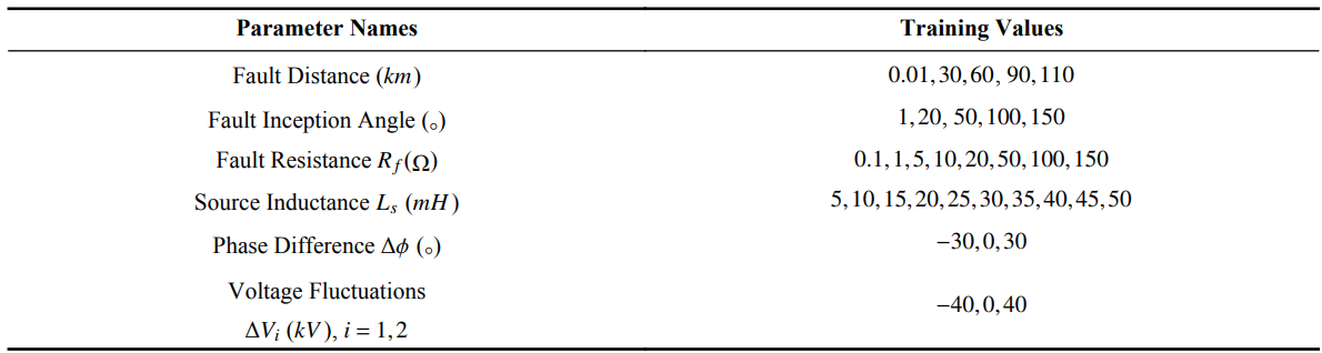
Table 1 Parameter values for the generation of training dataset.
The main goal of this paper is to present a fault detection and identification procedure based on the CNN, and assess its performances in terms of fault identification accuracy in high voltage TLs. This fault diagnosis system utilizes the voltage and current waveforms sensed from one end of a two-bus TL using current and voltage transformers. The distinguishing feature of this study is using the actual time-domain voltage and current signals instead of extracting frequency features based on signal processing methods such as FFT and WT. This important characteristic originates from the power of CNNs in handling large amount of time-series data. The CNN is sensitive to spatial features and therefore, can be the most reliable solution for TL fault diagnosis problem.The proposed CNN technique is assessed in terms of robustness against the possible variations of different factors such as fault types, fault distances, fault resistances, fault inception angles, and source inductance, as well as system operating points including voltage amplitudes and phases of all generators. Moreover, time delay analysis is carried out in this study to show that the detection, identification, and location estimation times are within the IEEE timing standard [47]. It should be noted that the effect of noises on fault identification is also investigated.
The contributions of this work are outlined as follows:
• The design of a CNN for the fault detection and identification problems in a transmission line based on the time-series signals without applying FFT or WT, which results in a highly robust performance.
• THe robustness analysis against alterations of fault resistance, fault inception angles, source inductance, phase difference between two connected buses, bus voltage fluctuations, and measurement noise for the CNN.
• The time delay analysis (cumulative detection and identification delays) based on the IEEE timing standard [47] for the CNN.
The rest of the paper is outlined as follows. Section 2 investigates a TL model and its waveform measurements. Section 3 presents the proposed CNN technique, generation of features, and fault detection and identification procedures. In Section 4, the simulation results are presented and the performance of the CNN is assessed in terms of cumulative detection and identification time delays, fault identification accuracy, and robustness against variations of the system parameters and measurement noise. Finally, the conclusion of our work is made in Section 5.
2. Transmission Line Model
The system used for this study is modelled as two three-phase generators connected by a 
 TL with a voltage rating of
 and frequency of
 as depicted in Figure 1.
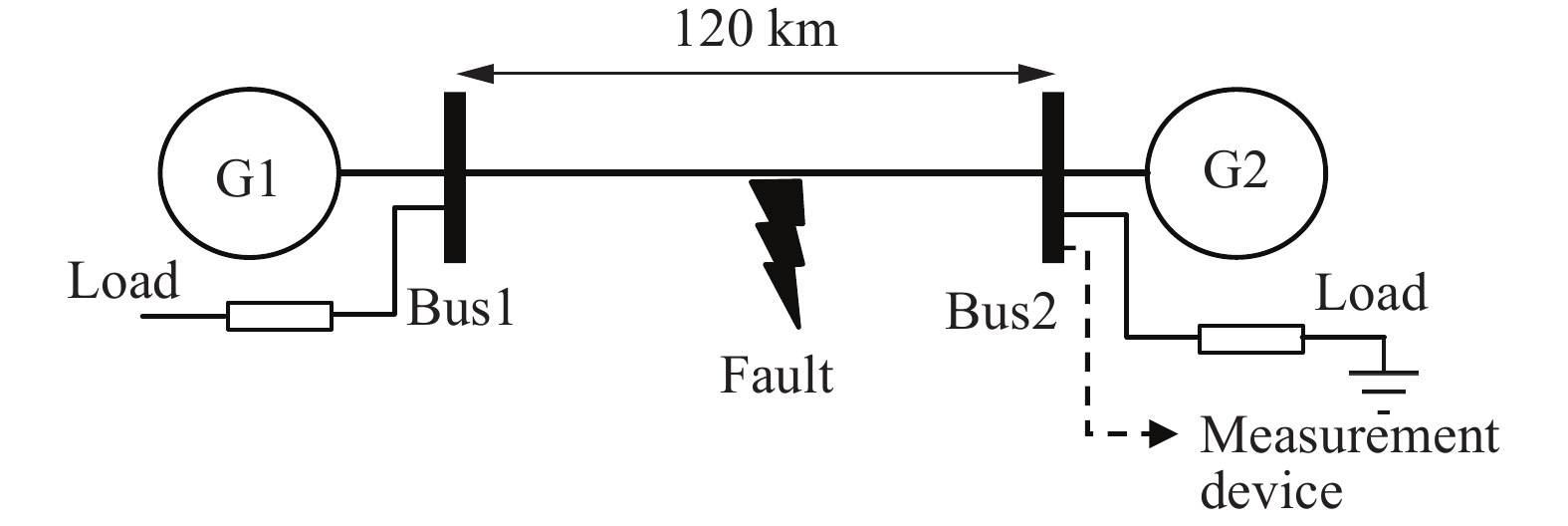
Figure 1. A two-bus power system.
The model is simulated in MATLAB Simulink’s Simscape Power System, and all the eleven fault scenarios are considered including no-fault, Line-to-Ground (LG), Line-to-Line (LL), Line-to-Line-to-Ground (LLG), and Line-to-Line-to-Line (LLL). The TL model parameters are shown in Table 2, and the values of the two generators and loads are given in Table 3. It should be pointed out that the transmission line model considered in this study is based on the IEEE39-Bus system which has 10 generators and 46 lines. In this work, only two of the generators have been considered with a three-phase transmission line in between.
Table 2 Nominal source and load parameters.
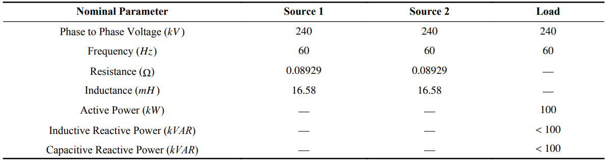
Table 3 Nominal parameters of TL.
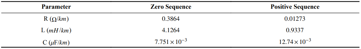
Figure 2 indicates faulty voltage and current waveforms of one end of the TL for an LL (phase A to phase B) fault at t = 0.5  . As observed in Figure 2(a), with the occurrence of the fault, the voltage amplitude of phases A and B decrease while the voltage amplitude of phase C remains unchanged. The current waveforms behave differently. Based on Figure 2(b), with the occurrence of the fault, the current amplitudes of phases A and B increase significantly, while it remains unchanged for phase C.
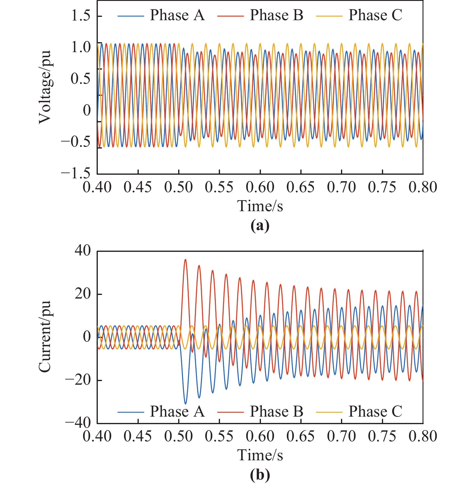
Figure2. The measured (a) voltages and (b) currents of one end of the TL for an LL (phase A to phase B) fault at t = 0.5 (sec)
3. Proposed Convolutional Neural Network (CNN) Technique
In this section, a brief introduction to the CNN used in this study is given, and its main characteristics are discussed. CNN, as a subset of deep learning methods, is mainly used for analyzing imagery datasets and image classification problems. The advantage of CNNs is that they can handle high dimensional datasets with higher speed, and are more efficient with minimum requirement for data preprocessing (no FFT, WT, WPT, or S-Transform (ST)) [ 48 ]. A CNN architecture consists of different layers including an input layer to obtain data from the datasets; convolutional layer to create a feature map for feature class probability prediction (this step is done by applying a filter that slides over the whole data block); pooling layers for down sampling the data; fully connected layers to flatten the outputs from prior layers to generate a single vector; and fully connected layers which involve weights, biases, and neurons to perform label prediction precisely by using feature analysis. The fully connected layers include a Softmax/Logistic layer, which resides at the end of fully connected layers (Logistic is used for binary classification and Softmax is for multi-classification), and an output layer to produce the final probabilities for class determination. The architecture of a CNN is a vital factor to determine its performance and efficiency. The way in which the layers are organized, the number of layers, the utilized elements in every layer, and their design affect the speed and accuracy of CNNs.
Studies on TL fault diagnosis problems that use CNNs are divided into two main categories. The first category includes those focusing on the image-based datasets taken from TLs above the ground [ 49 - 51 ]. The second category includes those that consider the generated time-series voltage and current signal waveforms from generators to be fed to the CNN. The details of the used CNN architecture can be found in reference [ 52 ], and this is only one architecture that can perform well with the generated dataset. Therefore, we have used a general form of CNN to show this generality and avoided using extra space for redundant material. In this study, a CNN architecture is designed based on LeNet5 [ 52 ], and the existing time-series dataset is considered as images generated to be classified. The utilized CNN consists of two convolution layers including  and
and  neurons and kernel sizes of
  and
and  , respectively, and uses ``relu'' activation function followed by a max pooling layer. Then a dropout layer with 0.25 value is added and its output is flattened by a flat layer. Moving towards the output layer, two dense layers with
  and
and  neurons, respectively, and another dropout with the value of 0.1 are included. The output layer is a dense layer with 16 neurons. The "adam" optimizer is used in this CNN. Also, the learning rate of this NN is equal to 0.1. This architecture generates 100% accuracy for TL fault identification, and the average of MSE for all types of faults is 0.006. Figure 3 shows the general architecture for CNNs. It should be noted that the CNN architecture shown in Figure 3 is just an architecture that can perform well with the generated dataset. Therefore, a general form of CNN is used to show this generality without using extra space for redundant material. For more details, please refer to [ 52 ].
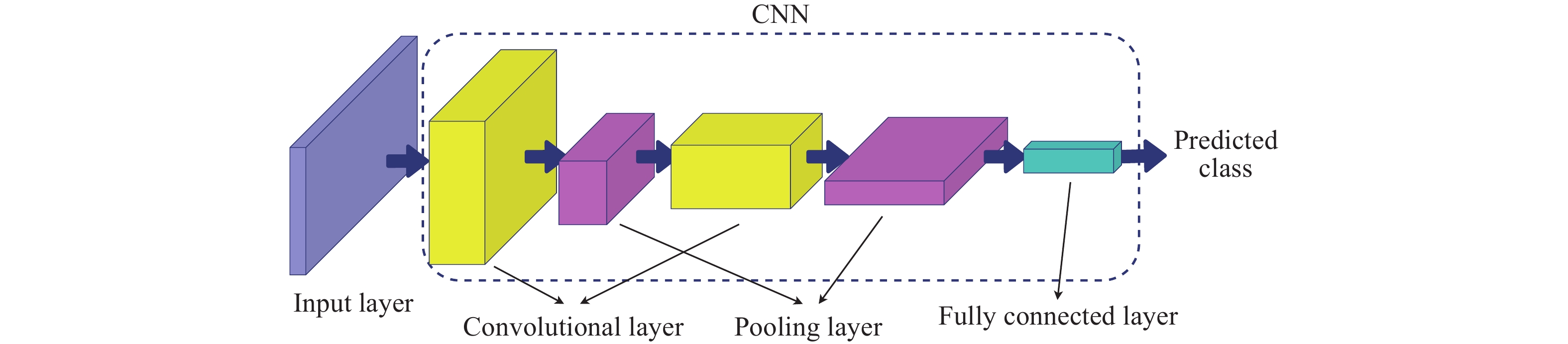
Figure 3. General architecture of a CNN.
3.1. Generation of Data
The data used for this study includes the waveforms of voltages and currents of the three phase voltages and currents recorded from one end of the TL. These waveforms consist of 1 cycle of the post-fault voltage and current signals which are fed directly to the detection and identification system. In order to generate training data, several variations in the fault model were considered that included fault type, location, inception time, source inductance, and resistance. In addition, different values for voltage amplitudes of the two generators as well as their phase difference were used to generate the training data. All these variations in the training data were considered to make the performance of the fault diagnosis system robust against variations in system operating points and fault model parameters. Table 1 shows the parameters that are changed for the generation of training dataset. In this table,  (
(  ) represents the voltage amplitude of generator
  , and
, and  is the phase difference between the two generators. The generated dataset includes 3,000,000 data points which are divided into 3 categories of training (70%), validation (15%), and test (15%).
There is an exception regarding detection of the faults involving ground. Distinguishing between LL and LLG faults cannot be accurately done by a fault diagnosis system only based on phase voltage and current signal measurements. Therefore, the zero-sequence current is calculated to provide a better indication of a ground fault since there is a considerable amount of zero-sequence current for an LLG fault. Such a current is calculated from the mean of the phase currents. Figures 4 and 5 show the zero-sequence current without and with a ground fault happening at 
 , respectively. As observed in Figure 4, when the ground is not involved in a fault, the zero-sequence current is almost zero. As shown in Figure 5, when the ground is involved, the amplitude oscillation increases significantly. Consequently, this significant difference is used in the NN training process for detection of ground involvement in faults.
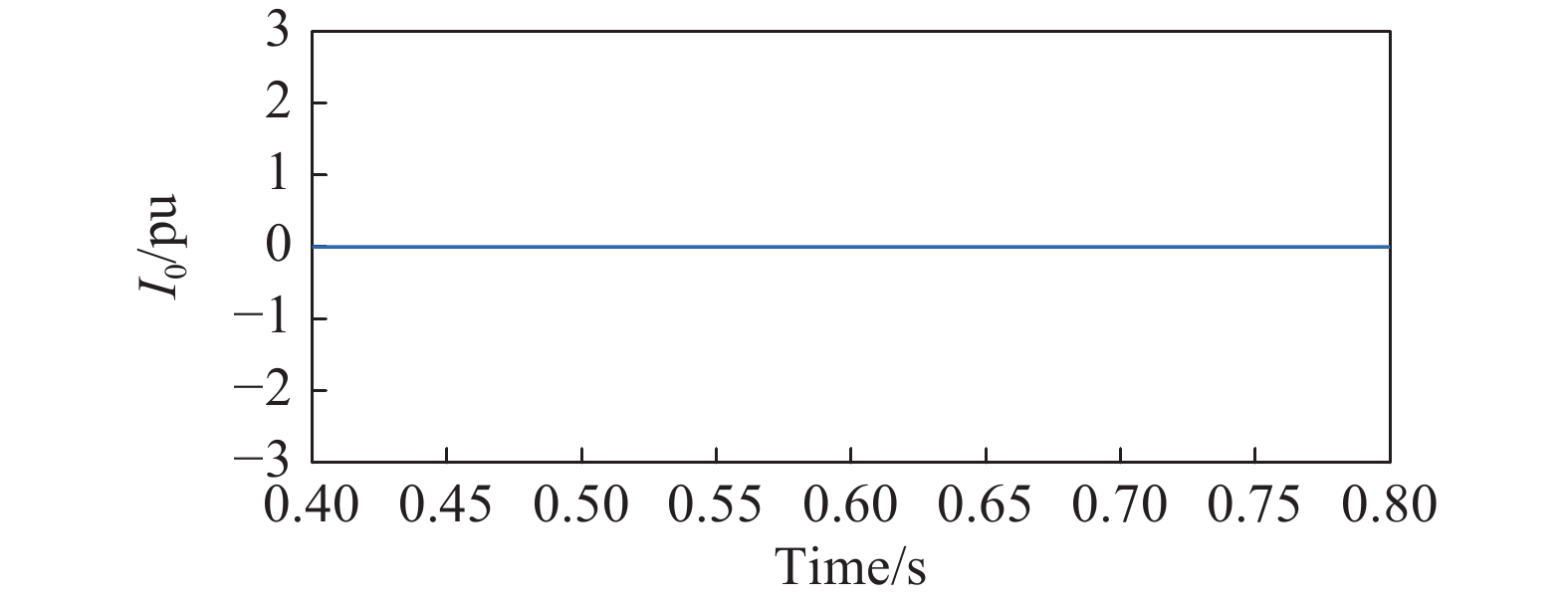
Figure4. I0 waveform when ground is not involved in an LL fault.
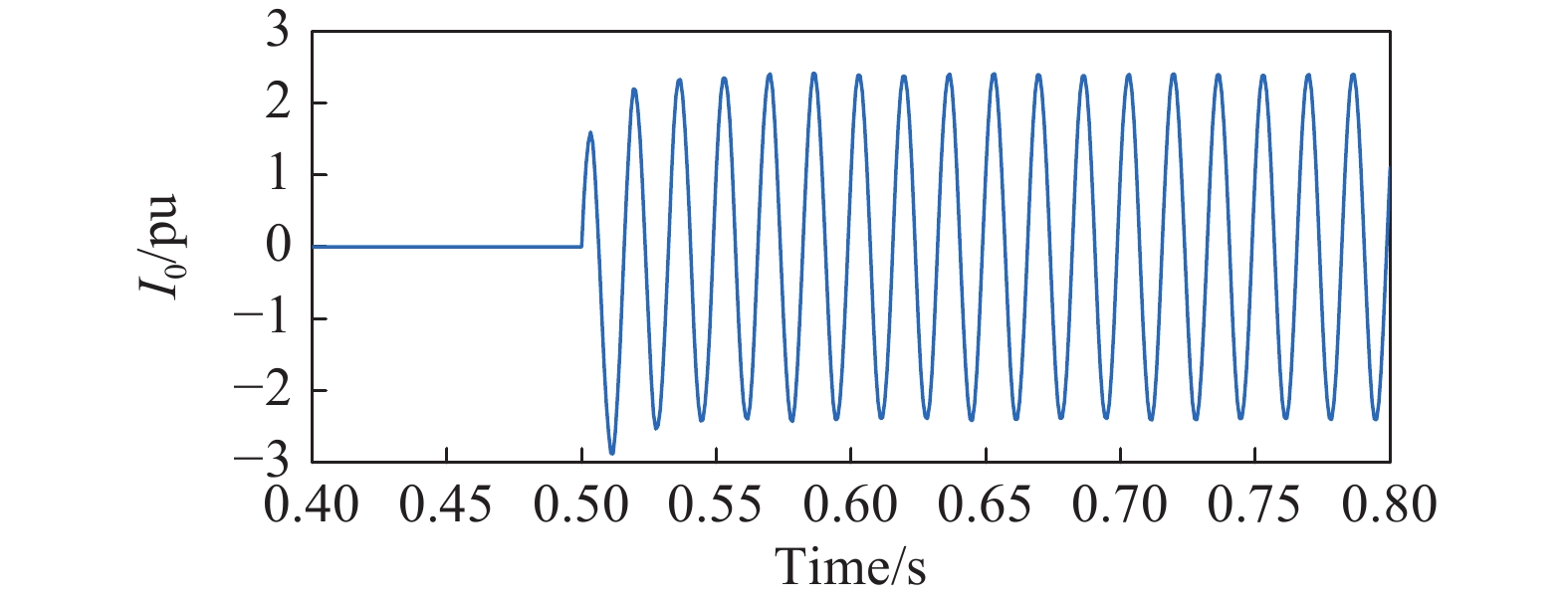
Figure5. I0 waveform when ground is involved in an LL fault (LLG).
3.2. Fault Detection and Identification
The first step in fault detection and identification is to acquire data from one end of the TL. As seen in Figure 1, the measurement device is placed at bus  . The current and voltage signals of the three-phase TL are recorded via a
  -sample time window with the sampling frequency of
 . For each window at every step, 1 cycle of the voltages and currents waveforms is recorded. In addition, the zero-sequence component is calculated for ground fault detection. The normalized extracted features are fed to the fault detection and identification system, which is based on CNN.
The fault detection and identification system generates 4 outputs. The first three outputs correspond to A, B, and C phases. The last output is associated with ground faults. In a non-faulty scenario, the values of all these outputs are zero. However, in a faulty situation, their values change. The time when at least one of these outputs (flags) switches to 1 is called the "detection time". At this point, the type of a fault has not been determined yet. In other words, other outputs may switch to  after waiting for more samples. Based on an extensive number of simulations for different fault scenarios for the CNN, it was found out that the longest identification was achieved within
  samples or
 from the fault occurrence time. Thus, we let the system wait for
  samples so that the type of a fault can be identified accurately. This
 (
(  samples) wait time is called "identification delay".
So far, the methodology of the fault diagnosis system and data generation has been explained. In the next section, the CNN method is applied to the generated voltage and current data with its performance analyzed.
4. Simulation Results
In this section, the simulation results for the performance analysis of fault detection, identification, and location estimation system in terms of time delays and robustness are presented. The following results are based on the model demonstrated in Figure 1 with the parameters specified in Tables 2 and 3 . It is to be noted that all the simulations are run on Matlab/Simulink using the real-time simulator OPAL-RT (OP5700). OP5700 includes a powerful computer which has a linux-based real-time operating system and its CPU specifications are Intel Xeon E5, 8 Cores,  , and
, and  Cache. The TL model shown in Figure 1 is implemented in the Simulink environment which is connected to RT-Lab software in OP5700. Then, the generated real-time faulty data is fed to the NN which is simulated in Matlab environment connected to RT-Lab. The fault detection and identification results are sent to a regular PC using a LAN cable and illustrated in Matlab environment in a Windows operating system as shown in Figure 6 .
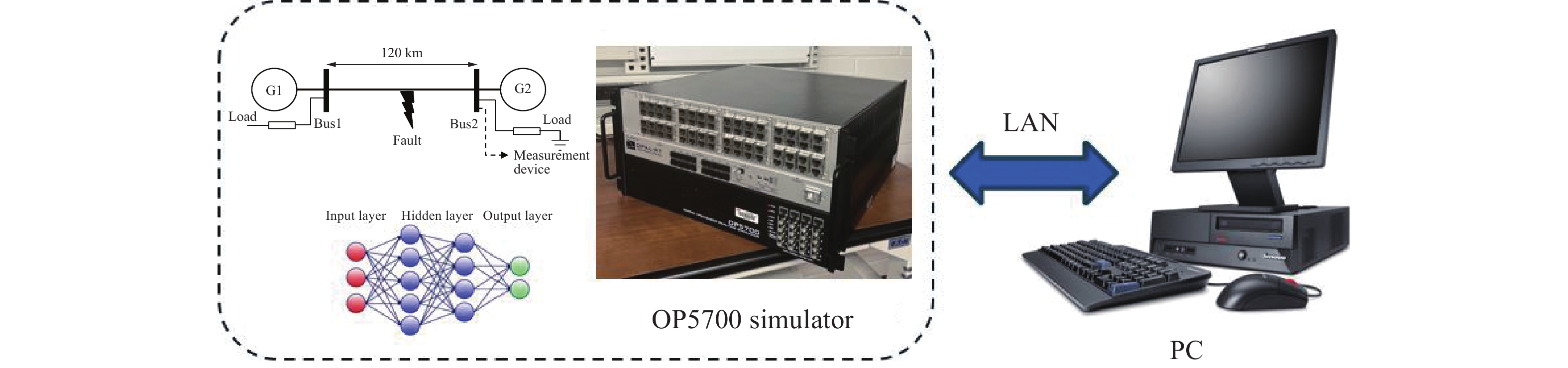
Figure 6. Real-time simulation using OP5700.
It is to be noted that for high voltage and current TLs, the three-phase voltage and current data are sensed by using current and voltage transformers which are placed in one end of the TL. Then, only 1 cycle time duration of the waveforms is considered as the time window to which the fault detection and identification schemes are applied.
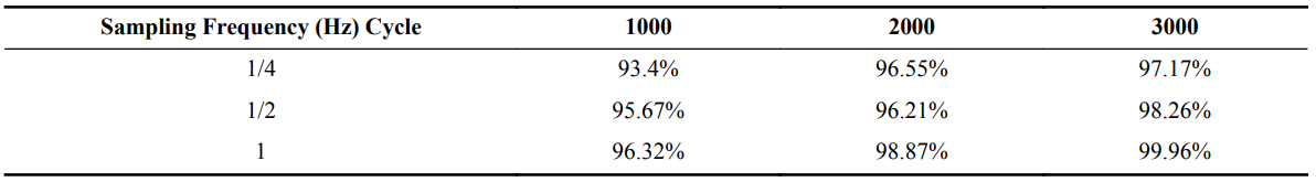
4.1. Sampling Frequency and Time Cycle Analysis
The first analysis is performed on the performance of the CNN technique with respect to different sampling frequencies and time cycles which play salient roles in the performance of the fault diagnosis system. As observed in Table 4, the CNN technique has the highest accuracy with the sampling frequency 
 and 1 cycle of data. Therefore, these two values are chosen for the rest of the analyses in the next subsection. However, choosing lower time cycles will also provide acceptable performance but with a faster detection time.
Table 4 Identification accuracy with respect to the sampling frequency and time cycles.
4.2. Robustness Analysis
The main parameters (uncertainties),which may change and impact the performance of a TL fault detection and identification system, are fault types, fault resistance (  ), phase difference between two sources (
  ), voltage fluctuations of the two sources (
  ), source inductance (
  ), and fault inception angle as included in Table 3. The fault identification system is trained to be robust against these parameter variations. For analyzing the detection and identification performance, the "accuracy" criterion is defined as the total number of correctly identified faulty or non-faulty scenarios divided by the total number of simulation experiments.
The performance of the fault diagnosis system is assessed in terms of fault types. The average accuracies of the fault diagnosis system for LL, LG, LLG, and LLL are 99.75%, 100%, 100%, and 96%, respectively. Based on these results, the performance for the faults involving ground (LG and LLG) is higher than LL and LLL faults, which proves the better identifiability of the ground-involved faults.
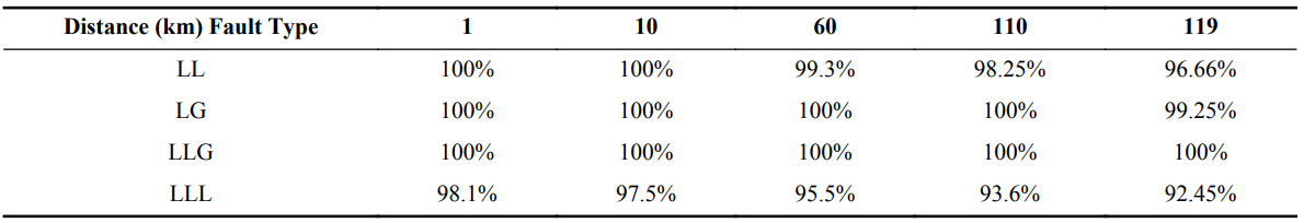
The performance of the proposed fault detection technique is also assessed in terms of fault distance from the measurement unit. Table 5 shows the performance of the CNN with respect to different fault distances. It is observed that the faults occurring close to the measurement unit are identified more accurately as compared to the ones occurring towards the other end of the TL. However, for the LLG fault, the accuracy is 100% regardless of where the fault happens throughout the TL. Moreover, the accuracy of the LLL fault is less than that of the rest of the fault types.
Table 5 Identification accuracy with respect to different fault types and distances.
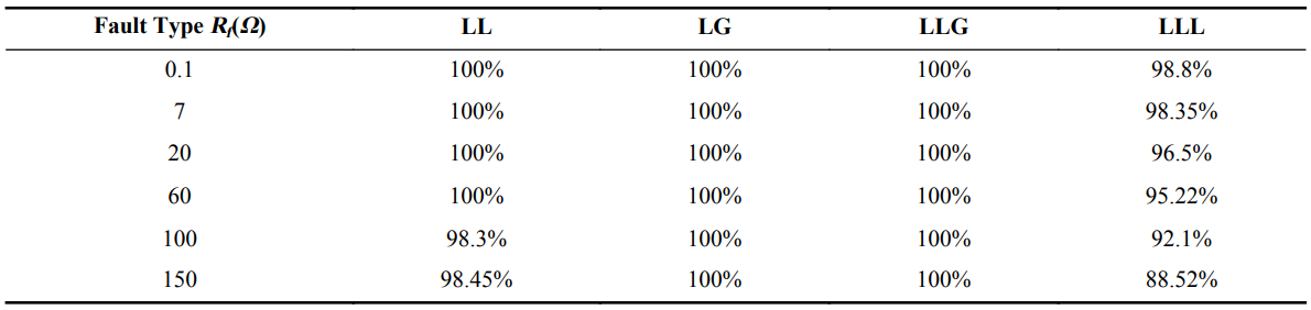
The fault identification and location estimation schemes must perform accurately for different fault resistances. Table 6 indicates the average accuracy of fault identification stage with respect to the variations of the fault resistance and for different fault types. The variations are considered to range from 
 to
to 
 [53]. It is seen that the CNN technique has the highest accuracy for LG and LLG fault types. For LL fault, the accuracy is high except for
 and
and 
 . The accuracy for the LLL fault type is less than the other fault types.
Table 6 Identification accuracy with respect to different fault types and resistances.
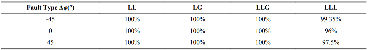
The phase difference between the two generators varies from time to time due to the various operating conditions. In Table 7, the average accuracies of the CNN technique are shown with respect to the variations of phase difference  between two generators that ranges from −45° to 45°. It is observed that the CNN method has an acceptable robustness against phase difference variations except for the fault LLL for which the accuracy has decreased.
Table 7 Identification accuracy with respect to different fault types and phase difference variations.
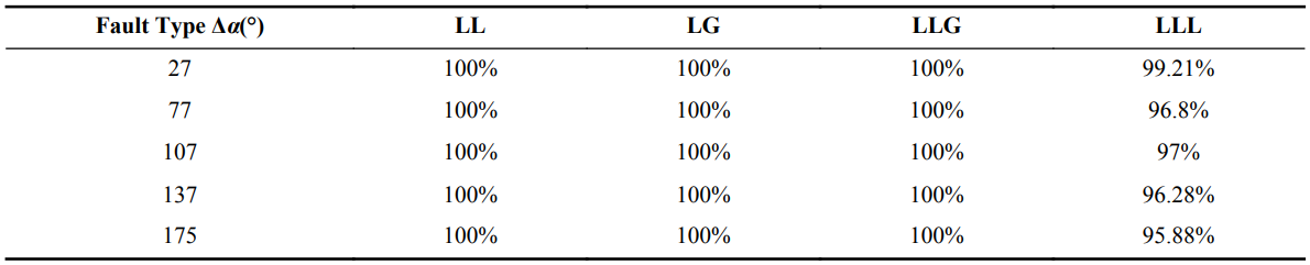
The fault diagnosis system must identify a fault with any inception angle. This parameter is varied from  to
to  [54]. Table 8 demonstrates the average accuracy of the CNN method with respect to the variations of the fault inception angle. It is observed that CNN has a good robustness except for the LLL fault type.
Table 8 Identification accuracy with respect to different fault types and inception angles.
The voltages of the two generators can change due to the different operating conditions of the generators. Based on the IEEE standard 1250 [55], the voltage fluctuations of a bus cannot exceed more than  of its nominal voltage level. In this study, the voltage changes increase beyond this limit in order to show the robustness of the fault diagnosis system with respect to this variation. The accuracy of the CNN method with respect to
  changes in both generator voltage amplitudes is 100% for all fault types except the LLL fault for which the accuracy is 97%.
The source inductance plays a prominent role in the shape of faulty waveforms, which negatively affects the estimated location of faults in TW approaches. The fault diagnosis system must be able to detect and identify the faults with the variations of source inductances. The accuracy of the CNN method with respect to  changes in both generator inductances is 100% for all fault types except the LLL fault for which the accuracy is 98.6%.
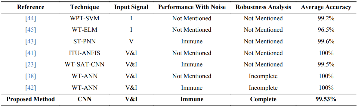
Table 9 illustrates the performance comparison of the proposed approach in this study with other techniques in the literature. Contrary to the proposed approach in this paper, all of the techniques in the literature have used feature extraction procedures such as WPT, WT, and ST to generate data for their classifiers. Moreover, although the approaches proposed in [38, 41, 43], and [42] have a better accuracy compared to the proposed approach, their robustness analyses have not been performed completely, and hance their performances may not be robust.
Table 9 Fault identification performance comparison among the proposed approach in this paper and the other techniques in the literature (I: Current and V: Voltage).
4.3. Effect of Noise
In real scenarios, the measurement noise in power systems may affect the accuracy of the fault diagnosis system. In order to assess the robustness of the fault detection and identification system against noises, a Gaussian noise is added to the measurement data (voltages and currents) so that the signal to noise ratio is 
 . Based on extensive simulations, the average fault identification accuracy subject to the Gaussian noise is
  . The identification accuracy without noises is shown to be
  in Table 9. This result indicates that the Gaussian noise has a negligible impact on the identification accuracy of our proposed method.
4.4. Time Delay Analysis
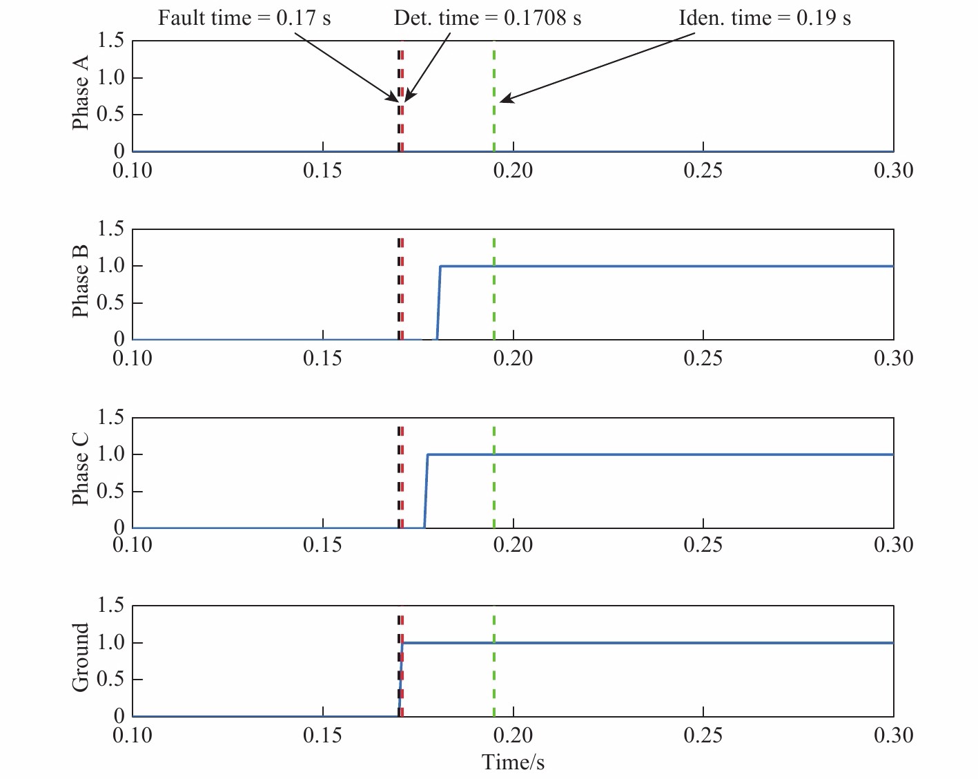
The faults must be detected and identified before the tripping relays and circuit breakers start to disconnect a faulty section of the TL. According to the IEEE timing standard [47], this time interval is between  to
to 
 from the occurrence of a fault. Figure 7 demonstrates the detection and identification times/delays of a BCG fault using our proposed CNN technique. It also indicates the time evolution of the detection and identification processes after the occurrence of a fault. The detection and identification delays are
 and
and 
 , respectively. This result confirms that the CNN-based fault diagnosis system proposed in this paper is capable of detecting and identifying faults well before the circuit breakers disconnect the faulty region of the TL.

Figure7. CNN-based fault diagnosis: Fault detection "Det." and identification ("Iden."), and their associated times/delays.
5. Conclusion
In this work, the problem of fault detection and identification for TLs using the CNN is studied. The acquired data includes the phase current and voltage waveforms measured from one end of the TL. One contribution of this paper is to use time-based voltage and current data instead of extracting data features using FFT, WT, and ST. In addition, the robustness of the proposed detection and identification technique against the changes of parameters/factors in a TL, namely, the fault type, fault distance, phase difference between the two buses, fault resistance, fault inception angle, source inductance, bus voltage amplitude variation, and noise level is analyzed. In addition, a time delay analysis is performed to guarantee that this method can successfully complete its task within the desired time window based on the IEEE timing standard [ 47 ] before the tripping relays and circuit breakers disconnect the TL. A few limitations regarding this method include retraining the NNs according to the changes in the TL model characteristics such as the voltage and length. For example, since the CNN in this study is trained for 240 (kV), it cannot be used to detect faults for a 110 (kV) TL. One solution to address such limitations is to take advantage of other novel deep learning techniques such as transfer learning [ 56 - 65 ], which remove the requirement to train the network all over again. In other words, we can reuse the trained model for similar TLs with various characteristics [ 62 ], which is one of our future research directions.
Author Contributions: S. Mohsen Azizi: conceptualization; Fatemeh Mohammadi Shakiba: Methodology; Fatemeh Mohammadi Shakiba and Milad Shojaee: software; Fatemeh Mohammadi Shakiba and Milad Shojaee: formal analysis; Fatemeh Mohammadi Shakiba: investigation; S. Mohsen Azizi: resources; Fatemeh Mohammadi Shakiba: data curation; Fatemeh Mohammadi Shakiba: writing—original draft preparation; Mengchu Zhou: writing—review and editing; Fatemeh Mohammadi Shakiba: visualization; Mengchu Zhou: supervision; Mengchu Zhou: project administration; S. Mohsen Azizi and Mengchu Zhou: funding acquisition. All authors have read and agreed to the published version of the manuscript.
Funding: This project is in part supported by 2022 Lam Research Foundation’s Unlock Ideas Program and FDCT(Fundo para o Desenvolvimento das Ciencias e da Tecnologia) under Grant No. 0047/2021/A1.
Conflicts of Interest: The authors declare no conflict of interest.
References
- Kumar, A.N.; Sanjay, C.; Chakravarthy, M.; et al, A single-ended directional relaying scheme for double-circuit transmission line using fuzzy expert system. Complex Intell. Syst., 2020, 6: 335−346.
- Raza, A.; Benrabah, A.; Alquthami, T.; et al, A review of fault diagnosing methods in power transmission systems. Appl. Sci., 2020, 10: 1312.
- Yusuff, A.A.; Jimoh, A.A.; Munda, J.L, Fault location in transmission lines based on stationary wavelet transform, determinant function feature and support vector regression. Electr. Power Syst. Res., 2014, 110: 73−83.
- Livani, H.; Evrenosoglu, C.Y, A machine learning and wavelet-based fault location method for hybrid transmission lines. IEEE Trans. Smart Grid, 2014, 5: 51−59.
- Khodaparast, J.; Khederzadeh, M, Three-phase fault detection during power swing by transient monitor. IEEE Trans. Power Syst., 2015, 30: 2558−2565.
- Guillen, D.; Paternina, M.R.A.; Ortiz-Bejar, J.; et al, Fault detection and classification in transmission lines based on a PSD index. IET Gener. Trans. Distrib., 2018, 12: 4070−4078.
- Khan, A.Q.; Ullah, Q.; Sarwar, M.; et al, Transmission line fault detection and identification in an interconnected power network using phasor measurement units. IFAC-PapersOnLine, 2018, 51: 1356−1363.
- Ziegler, G.
Numerical Distance Protection: Principles and Applications , 4th ed. Wiley: Hoboken, NJ, USA, 2011. - Asprou, M.; Kyriakides, E.; Albu, M. The effect of PMU measurement chain quality on line parameter calculation. In
2017 IEEE International Instrumentation and Measurement Technology Conference (I2MTC), Turin, Italy, 22–25 May 2017 ; IEEE: Turin, Italy, 2017; pp. 1–6. doi: 10.1109/I2MTC.2017.7969757 - Jana, S.; De, A, A novel zone division approach for power system fault detection using ANN-based pattern recognition technique. Can. J. Electr. Comput. Eng., 2017, 40: 275−283.
- Li, W.L.; Monti, A.; Ponci, F, Fault detection and classification in medium voltage DC shipboard power systems with wavelets and artificial neural networks. IEEE Trans. Instrum. Meas., 2014, 63: 2651−2665.
- Li, H.F.; Hu, G.Z.; Li, J.Q.; et al., Intelligent fault diagnosis for large-scale rotating machines using binarized deep neural networks and random forests. IEEE Trans. Autom. Sci. Eng., 2022, 19: 1109−1119.
- Ravikumar, B.; Thukaram, D.; Khincha, H.P, Application of support vector machines for fault diagnosis in power transmission system. IET Gener. Trans. Distrib., 2008, 2: 119−130.
- Swetapadma, A.; Yadav, A, A novel decision tree regression-based fault distance estimation scheme for transmission lines. IEEE Trans. Power Delivery, 2017, 32: 234−245.
- Upendar, J.; Gupta, C.P.; Singh, G.K, Statistical decision-tree based fault classification scheme for protection of power transmission lines. Int. J. Electr. Power Energy Syst., 2012, 36: 1−12.
- Chen, Y.Q.; Fink, O.; Sansavini, G, Combined fault location and classification for power transmission lines fault diagnosis with integrated feature extraction. IEEE Trans. Ind. Electron., 2018, 65: 561−569.
- Xie, Y.Y.; Li, C.J.; Lv, Y.J.; et al, Predicting lightning outages of transmission lines using generalized regression neural network. Appl. Soft Comput., 2019, 78: 438−446.
- Thwe, E.P.; Oo, M.M, Fault detection and classification for transmission line protection system using artificial neural network. J. Electr. Electron. Eng., 2016, 4: 89−96.
- Shakiba, F.M. CMOS Based Implementation of Hyperbolic Tangent Activation Function for Artificial Neural Network. Master’s Thesis, Southern Illinois University, Carbondale, USA, 2018.
- Shakiba, F.M.; Zhou, M, Novel analog implementation of a hyperbolic tangent neuron in artificial neural networks. IEEE Trans. Ind. Electron., 2021, 68: 10856−10867.
- Koley, E.; Yadav, A.; Thoke, A.S, A new single-ended artificial neural network-based protection scheme for shunt faults in six-phase transmission line. Int. Trans. Electr. Energy Syst., 2015, 25: 1257−1280.
- Abdel-Aziz, A.M.; Hasaneen, B.M.; Dawood, A.A, Detection and classification of one conductor open faults in parallel transmission line using artificial neural network. Int. J. Sci. Res. Eng. Trends, 2016, 2: 139−146.
- Fahim, S.R.; Sarker, Y.; Sarker, S.K.; et al, Self attention convolutional neural network with time series imaging based feature extraction for transmission line fault detection and classification. Electr. Power Syst. Res., 2020, 187: 106437.
- Fuada, S.; Shiddieqy, H.A.; Adiono, T.; et al, A high-accuracy of transmission line faults (TLFs) classification based on convolutional neural network. Int. J. Electron. Telecommun., 2020, 66: 655−664.
- Rai, P.; Londhe, N.D.; Raj, R.; et al, Fault classification in power system distribution network integrated with distributed generators using CNN. Electr. Power Syst. Res., 2021, 192: 106914.
- Costa, F.B.; Monti, A.; Lopes, F.V.; et al, Two-terminal traveling-wave-based transmission-line protection. IEEE Trans. Power Delivery, 2017, 32: 1382−1393.
- Hasheminejad, S.; Seifossadat, S.G.; Razaz, M.; et al, Ultra-high-speed protection of transmission lines using traveling wave theory. Electr. Power Syst. Res., 2016, 132: 94−103.
- Yadav, A.; Swetapadma, A, Enhancing the performance of transmission line directional relaying, fault classification and fault location schemes using fuzzy inference system. IET Gener. Trans. Distrib., 2015, 9: 580−591.
- Rahmati, A.; Adhami, R. A fault detection and classification technique based on sequential components. In
2013 IEEE Industry Applications Society Annual Meeting, Lake Buena Vista, FL, USA, 06–11 October 2013 ; IEEE: Lake Buena Vista, FL, USA, 2013; pp. 1–5. doi: 10.1109/IAS.2013.6682618 - Chakraborty, C.; Verma, V, Speed and current sensor fault detection and isolation technique for induction motor drive using axes transformation. IEEE Trans. Ind. Electron., 2015, 62: 1943−1954.
- Ohrstrom, M.; Soder, L, Fast protection of strong power systems with fault current limiters and PLL-aided fault detection. IEEE Trans. Power Delivery, 2011, 26: 1538−1544.
- Pei, X.Y.; Pang, H.; Li, Y.F.; et al, A novel ultra-high-speed traveling-wave protection principle for VSC-based DC grids. IEEE Access, 2019, 7: 119765−119773.
- Cervantes, M.; Kocar, I.; Mahseredjian, J.; et al. A traveling wave based fault location method using unsynchronized current measurements. In
2019 IEEE Power & Energy Society General Meeting (PESGM), Atlanta, GA, USA, 04–08 August 2019 ; IEEE: Atlanta, GA, USA, 2019; pp. 1. doi: 10.1109/PESGM40551.2019.8974132 - Ritzmann, D.; Wright, P.S.; Holderbaum, W.; et al, A method for accurate transmission line impedance parameter estimation. IEEE Trans. Instrum. Meas., 2016, 65: 2204−2213.
- Pegoraro, P.A.; Brady, K.; Castello, P.; et al, Line impedance estimation based on synchrophasor measurements for power distribution systems. IEEE Trans. Instrum. Meas., 2019, 68: 1002−1013.
- Waters, D.H.; Hoffman, J.; Kumosa, M, Monitoring of overhead transmission conductors subjected to static and impact loads using fiber Bragg grating sensors. IEEE Trans. Instrum. Meas., 2019, 68: 595−605.
- Kazim, M.; Khawaja, A.H.; Zabit, U.; et al, Fault detection and localization for overhead 11-kV distribution lines with magnetic measurements. IEEE Trans. Instrum. Meas., 2020, 69: 2028−2038.
- Koley, E.; Kumar, R.; Ghosh, S, Low cost microcontroller based fault detector, classifier, zone identifier and locator for transmission lines using wavelet transform and artificial neural network: A hardware co-simulation approach. Int. J. Electr. Power Energy Syst., 2016, 81: 346−360.
- Gururajapathy, S.S.; Mokhlis, H.; Illias, H.A, Fault location and detection techniques in power distribution systems with distributed generation: A review. Renewable Sustainable Energy Rev., 2017, 74: 949−958.
- Department of energy. 2018. Available online:https://www.energy.gov/ne/articles/department-energy-report-explores-us-advanced-small-modular-reactors-boost-grid(access on 6 October 2022).
- Reddy, M.J.B.; Gopakumar, P.; Mohanta, D.K, A novel transmission line protection using DOST and SVM. Eng. Sci. Technol. Int. J., 2016, 19: 1027−1039.
- Koley, E.; Verma, K.; Ghosh, S, An improved fault detection classification and location scheme based on wavelet transform and artificial neural network for six phase transmission line using single end data only. SpringerPlus, 2015, 4: 551.
- Roy, N.; Bhattacharya, K, Detection, classification, and estimation of fault location on an overhead transmission line using S-transform and neural network. Electr. Power Compon. Syst., 2015, 43: 461−472.
- Ray, P.; Mishra, D.P, Support vector machine based fault classification and location of a long transmission line. Eng. Sci. Technol. Int. J., 2016, 19: 1368−1380.
- Malathi, V.; Marimuthu, N.S.; Baskar, S.; et al, Application of extreme learning machine for series compensated transmission line protection. Eng. Appl. Artif. Intell., 2011, 24: 880−887.
- Chen, K.J.; Hu, J.; He, J.L, Detection and classification of transmission line faults based on unsupervised feature learning and convolutional sparse autoencoder. IEEE Trans. Smart Grid, 2018, 9: 1748−1758.
- Lukach, D.; Taylor, R, Transmission line applications of directional ground overcurrent relays. IEEE Power Energy Soc., 2014, 10.
- Kiruthika, M.; Bindu, S, Classification of electrical power system conditions with convolutional neural networks. Eng. Technol. Appl. Sci. Res., 2020, 10: 5759−5768.
- Lei, X.S.; Sui, Z.H, Intelligent fault detection of high voltage line based on the faster R-CNN. Measurement, 2019, 138: 379−385.
- Wang, Y.H.; Li, Q.Q.; Chen, B, Image classification towards transmission line fault detection via learning deep quality-aware fine grained categorization. J. Vis. Commun. Image R., 2019, 64: 102647.
- Dai, Z.Y.; Yi, J.J.; Zhang, Y.J.; et al, Fast and accurate cable detection using CNN. Appl. Intell., 2020, 50: 4688−4707.
- Dong, J.J.; Chen, W.; Xu, C. Transmission line detection using deep convolutional neural network. In
2019 IEEE 8th Joint International Information Technology and Artificial Intelligence Conference (ITAIC), Chongqing, China, 24–26 May 2019 ; IEEE: Chongqing, China, 2019; pp. 977–980. doi: 10.1109/ITAIC.2019.8785845 - Moravej, Z.; Pazoki, M.; Khederzadeh, M, New pattern-recognition method for fault analysis in transmission line with UPFC. IEEE Trans. Power Delivery, 2015, 30: 1231−1242.
- Swetapadma, A.; Yadav, A, A novel single-ended fault location scheme for parallel transmission lines using k-nearest neighbor algorithm. Comput. Electr. Eng., 2018, 69: 41−53.
- IEEE guide for identifying and improving voltage quality in power systems. IEEE Std 1250-2011, 2018. Available online: https://ieeexplore.ieee.org/document/8532376(access on 10 October 2022)
- Zhang, W.J.; Wang, J.C.; Lan, F.P.; et al, Dynamic hand gesture recognition based on short-term sampling neural networks. IEEE/CAA J. Autom. Sin., 2021, 8: 110−120.
- Harford, S.; Karim, F.; Darabi, H, Generating adversarial samples on multivariate time series using variational autoencoders. IEEE/CAA J. Autom. Sin., 2021, 8: 1523−1538.
- Luo, X.D.; Wen, X.H.; Zhou, M.C.; et al, Decision-tree-initialized dendritic neuron model for fast and accurate data classification. IEEE Trans. Neural Netw. Learn. Syst., 2022, 33: 4173−4183.
- Huang, Z.H.; Yang, S.Z.; Zhou, M.C.; et al, Feature map distillation of thin nets for low-resolution object recognition. IEEE Trans. Image Process., 2022, 31: 1364−1379.
- Ohata, E.F.; Bezerra, G.M.; das Chagas, J.V.S.; et al, Automatic detection of COVID-19 infection using chest X-ray images through transfer learning. IEEE/CAA J. Autom. Sin., 2021, 8: 239−248.
- Yao, S.Y.; Kang, Q.; Zhou, M.C.; et al, A survey of transfer learning for machinery diagnostics and prognostics. Artif. Intell. Rev., 2022: 1−52.
- Shakiba, F.M.; Shojaee, M.; Azizi, S.M.; et al, Generalized fault diagnosis method of transmission lines using transfer learning technique. Neurocomputing, 2022, 500: 556−566.
- Shakiba, F.M.; Azizi, S.M.; Zhou, M.C., A transfer learning-based method to detect insulator faults of high-voltage transmission lines via aerial images: Distinguishing intact and broken insulator images. IEEE Syst. Man Cybern. Mag., 2022, 8: 15−25.
- Shakiba, F.M.; Azizi, S.M.; Zhou, M.C.; et al. Application of machine learning methods in fault detection and classification of power transmission lines: a survey.
Artif. Intell. Rev .2022 , in press. doi:10.1007/s10462-022-10296-0 - Shakiba, F.M.; Shojaee, M.; Azizi, S.M.; et al. Robustness analysis of generalized regression neural network-based fault diagnosis for transmission lines. In 2022 IEEE International Conference on Systems, Man, and Cybernetics, Prague, Czech Republic, 09–12 October 2022; IEEE: Prague, Czech Republic, 2022; pp. 131–136. doi:10.1109/SMC53654.2022.9945342