
The assessment of student performance has a significant impact on instructional strategies, individualised learning, and academic achievement in the setting of higher education [1, 2]. English language competency stands out among the many academic courses as a critical set of skills required for academic success, career advancement, and communication in today’s globalised society [3]. Using advanced predictive modelling approaches to anticipate and understand student performance in college English courses is becoming more and more popular as institutions work to improve their teaching strategies and maximise student outcomes [4, 5].
The subject of educational data analysis has seen a revolution with the introduction of machine learning and statistical modelling, which have provided powerful tools for deriving insightful conclusions from large, complicated datasets [6, 7]. Gaussian process model classification (GPMC) has become a popular and efficient method for predictive modelling in a variety of fields, such as engineering, finance, and healthcare, in recent years. Gaussian process models present an attractive option for forecasting student outcomes in educational settings because they offer a versatile framework that takes into account non-linear correlations and uncertainty estimation.
Because language learning and evaluation are complex processes, there are a number of issues with predictive modelling college English test scores [8]. Predicting student performance in English courses requires navigating the complexities of language acquisition, cognitive capacities, and socio-cultural aspects, in contrast to deterministic models that rely on established rules or assumptions. The intricate and naturally fluctuating nature of language proficiency poses a challenge in creating oversimplified forecasting models that accurately represent the subtleties of students’ learning paths [9].
Furthermore, written assignments, oral presentations, and standardised examinations are frequently used in traditional methods of evaluating student performance in college English courses [9]. These methods may provide only a limited amount of information regarding the comprehensive development of language skills. Traditional evaluation techniques might not take into consideration the dynamic interactions that exist between educational interventions, individual learning styles, and language competency [10, 11].
The diversity of student populations and institutional circumstances must be taken into account when predicting modelling college English scores, in addition to the challenges inherent in language learning and evaluation [11]. English language competency and academic accomplishment can be impacted by a variety of factors, including the linguistic backgrounds, socioeconomic level, and prior educational experiences of the students enrolled in universities. Additionally, variations in curriculum frameworks, instructional strategies, and institutional resources all add to the variation in student performance seen in various academic contexts [12].
When it comes to forecasting college English scores, Gaussian process model classification provides a convincing framework that takes into account the particularities of educational data, even in the face of difficulties and complexities. Gaussian process models offer a non-parametric method of modelling complex interactions without predetermined hypotheses, in contrast to typical regression or classification models that make strict assumptions about data distributions and functional forms. Gaussian process model categorization allows for the uncertainty and variability that are inherent in predicting student performance, allowing for more accurate and detailed forecasts [13, 14]. This is achieved by treating predictions as distributions across probable outcomes.
This study intends to create a thorough predictive modelling framework for predicting college English results using Gaussian process model classification in light of the aforementioned potential and limitations [15]. The primary objectives of this research effort are as follows:
Examining how well the Gaussian process model categorization predicts college English course achievement for students.
Investigating how predictive modelling can be used to inform curriculum creation, student support services, and instructional practices in higher education settings [16]. Through the pursuit of these goals, this research aims to further our knowledge of predictive modelling approaches in the context of educational evaluation and support current initiatives to maximise student performance and foster academic success in college English courses. This research project attempts to provide insightful analysis and practical suggestions for teachers, administrators, and legislators looking to maximise the benefits of data-driven approaches in higher education through methodological innovation and empirical validation [17].
The Naive Bayes method is a classification strategy that is predicated on the feature conditional independence assumption and the Bayes theorem. Based on the premise of conditional independence of features, the joint probability distribution of inputs and outputs for a particular training dataset is first learned; using this model, then, using Bayes’ Theorem, the output Y with the largest posterior probability for a given input X is determined [18].
Assume that \({A_i}(1 \le i \le n)\) events meet:
Since the two cannot coexist when \(i = j\), there are \({A_i} \cap {A_j} = \emptyset\);
\({\rm{P}}\left( {{A_i}} \right) > 0(1in){\rm{ }}\);
Example area \({\rm{ }}\Omega = \bigcup\limits_{i = 1}^n {{A_i}}\);
Then, the following equation is true for any event \(B\):
\[\label{e1}\tag{1} {\rm{P}}\left( {{A_i}\mid {\rm{B}}} \right) = {{{\rm{P}}\left( {{A_i}} \right) \times {\rm{P}}\left( {{\rm{B}}\mid {A_i}} \right)} \over {\sum\limits_{i = 1}^n P \left( {{A_i}} \right) \times {\rm{P}}\left( {{\rm{B}}\mid {A_i}} \right)}},i = 1,2 \cdots \cdots n.\] “Likelihood value” (\({\rm{P}}\left( {{A_i}\mid {\rm{B}}} \right)\)) is not a probability density, but rather the likelihood that event B will occur given that event \(A_i\) occurs [19].
Assume that \({{\rm{B}}_j}(1 \le j \le m)\) events meet:
Since the two don’t depend on one another, when \(i \ne j\) , there are \[\label{e2}\tag{2} P\left( {{B_i}\mid {B_j}} \right) = P\left( {{B_i}} \right){\rm{ or }}P\left( {{B_j}\mid {B_i}} \right) = P\left( {{B_j}} \right).\]
\(P\left( {{B_j}} \right) > 0(1 \le j \le m)\), the following formula is established:
\[\label{e3}\tag{3} {\rm{P}}\left( {{A_i}\mid {B_1}{B_2} \ldots \ldots {B_m}} \right) = {{{\rm{P}}\left( {{A_i}} \right) \times \prod\limits_{j = 1}^m P \left( {{B_j}\mid {A_i}} \right)} \over {\sum\limits_{i = 1}^n P \left( {{A_i}} \right) \times \prod\limits_{j = 1}^m P \left( {{B_j}\mid {A_i}} \right)}},i = 1,2 \cdots \cdots n.\]
Only the numerator portion of Eq. (2) can be computed for classification because the denominator is fixed. The combined probability distribution of every \({A_i}(1 \le i \le n)\) and \({A_j}(1 \le j \le m)\) is computed, and the prediction result for a given input value is the maximum of n values. This is the prediction process using the fundamental Bayes formula.
Between the polynomial and Bernoulli models, the polynomial model is the only one that is appropriate to the case of discrete characteristics. The Gaussian model, the polynomial model, and the Bernoulli model are the three models that are commonly used for the plain Bayesian algorithm [6]. Although the Gaussian model is intended to operate with continuous feature variables, it requires that the feature data of each dimension has a normal distribution. The likelihood value of each dimension can be calculated from the feature values by taking the mean and variance of each dimension. This allows the probability density value of each dimension to be determined.
For the specific problem of grade prediction, \({B_j}\) is regarded as a continuous-valued attribute with a Gaussian distribution in the fundamental Bayesian formulation.Assume that \(P\left( {{B_j}\mid {A_i}} \right)\ \sim N\left( {{\mu _{{A_i},j}},\sigma _{{A_i},j}^2} \right)\), \({\mu _{{A_i},j}}\) and \(\sigma _{{A_i},j}^2\) are the \(j\)-th attribute’s mean and variance for the value of the \(A_i\)-th sample, respectively.
\(P\left( {{B_j}\mid {A_i}} \right)\)’s probability density function is then: \[\label{e4}\tag{4} P\left( {{B_j}\mid {A_i}} \right) = {1 \over {\sqrt {2\pi } {\sigma _{{A_i}j}}}}\exp \left( { – {{{{\left( {{B_j} – {\mu _{{A_i}j}}} \right)}^2}} \over {2\sigma _{{A_i}j}^2}}} \right).\] Here’s how to get the Gaussian plain Bayes classifier: \[\label{e5}\tag{5} {h_{nb}}({\rm{B}}) = \arg {\max _{{A_i} \in y}}{\rm{P}}\left( {{A_i}} \right) \times \prod\limits_{j = 1}^m P \left( {{B_j}\mid {A_i}} \right),\] where the value entered \(B = \left( {{B_1},{B_2}, \ldots ,{B_m}} \right),{\rm{P}}\left( {{A_i}} \right)\) is the likelihood of the prior \({A_i}\) nd class of samples and \({h_{nb}}({\rm{B}})\) depicts the input value’s prediction.
Tables 1 and 2 present the findings from the survey utilised to gather the data samples, which included the typical college English quiz scores of 465 undergraduate students from the classes of 2018 to 2020. It is noted that the gathered data samples exhibit a number of traits; 1) It’s possible that some students did not take a particular test, in which case their results are recorded as 0; the typical test scores may be absent; 2) The scores on standard tests are typically higher than those on the final exam because they are likely the product of numerous repetitions by the students; 3) The tests vary in difficulty, which causes a significant variation in the test results. The data set possesses the qualities listed below. In light of the features of the data set given above, the following assumptions are made in this paper: Every feature is distinct from the others, meaning that the outcomes of the three tests don’t affect each other; each feature’s data set follows a normal distribution (that is, the student test data sets are continuous and follow a Gaussian distribution); and any missing data will be filled in by averaging the test results. The provided dataset has the formatas shown in Table 3.
| Number | Attributes | Characteristics |
| 1 | School | Name of the school in which the student is enrolled: (GP and MS) |
| 2 | Sex | Sex of students: (F: female; M: male) |
| 3 | Age | Age of students: (15 to 22 in Arabic numerals) |
| 4 | Address | Student’s home address: (U: urban; R: rural) |
| 5 | Famsize | Size of student’s family: (LE3: less than or equal to 3 persons; GT3: more than 3 persons) |
| 6 | Pstatus | Parental cohabitation (T: cohabitation; A: separation) |
| 7 | Medu | Mother’s education (0: no education; 1: primary education; 2: elementary education; 3: secondary education) |
| 8 | Fedu | Educational attainment of fathers in higher education) (0: no education; 1: primary education; 2: primary education; 3: secondary education) |
| 9 | Mjob | Mother’s work: higher education (teacher: ) teacher; health: doctor; services: service person; at home: at home; other: other |
| 10 | Fjob | Father’s work (teacher: teacher; health: doctor; services: service person; at home: at home; other: other) |
| 11 | Reason | Reasons for choosing a school ( close to home: close to home; school reputation: school reputation; course |
| 12 | Guardian preference | The student’s guardian prefers his/her course; (mother: mother;: other father): father; other: other) |
| 13 | Traveltime | Time spent travelling to school (1: less than 15 min; 2: 15 to 30 min; 3: 30 min to 1 h; 4: more than 1 h) |
| 14 | Studytime | Study time during the week (1: less than 2 h; 2: 2 h to 5 h; 3: 5 h to 10 h; 4: more than 10 h) |
| 15 | Failures | Number of past failures (1:1; 2:2; 3:3; 4:>3) |
| 16 | Schoolsup | Schools are supportive of education (yes: supportive; no: not supportive) |
| 17 | Famsup | Family support for education (yes: supportive; no: not supportive) |
| 18 | Paid | Whether classes are made up (yes: classes are made up; no: classes are not made up) |
| 19 | Activities | Participation in extracurricular activities (yes: yes; no: no) |
| 20 | Nursery | Attended kindergarten (yes: yes; no: no) |
| 21 | Higher | Whether they want to go to university (yes: up; no: not) |
| 22 | Interne | Whether you have internet access at home (yes: internet access; no: no internet access) |
| 23 | Romantic | Whether in a relationship (yes: in a relationship; no: not in a relationship) |
| 24 | Famrel | Good or bad family relationship (from poor to good, in descending order from 1 to 5) |
| 25 | Freetime | Free time after school (in descending order from 1 to 5) |
| Number | Attributes | Characteristics |
| 1 | School | GP( Gabriel Pereira) = 0; MS( Mousinho da Silveira)= 1 |
| 2 | sexuality | Female=0; Male=1 |
| 3 | Age | [15,22] |
| 4 | Home address | City=0; Rural=1 |
| 5 | Household size | No more than 3 people=0; More than 3 people=1 |
| 6 | Parental | cohabitation situationCohabitation=0; Separation=1 |
| 7 | Mother’s education level | Not attending school=0; Primary school=1; Primary education=2; Secondary education=3; Higher education=4 |
| 8 | Father’s education level | Not attending school=0; Primary school=1; Primary education=2; Secondary education=3; Higher education=4 |
| 9 | Mother’s work | Teacher=0; Medical care=1; Service industry=2; At home=3; Other=4 |
| 10 | Father’s job | Teacher=0; Medical care=1; Service industry=2; At home=3; Other=4 |
| 11 | Reasons for choosing a school | Near home=1; School reputation=2; Likes its course=3; Other=0 |
| 12 | Guardian | Mother=1; Father=2; Other=0 |
| 13 | Spending time on education | Less than 15 minutes=1; 15-30 minutes=2; 30 60 minutes=3; Greater than 60 minutes=4 |
| 14 | One week of study time | Less than 2 hours=1; 2-5 hours=2; 5-10 hours=3; Greater than 10 hours=4 |
| 15 | Past failures | 1 time=0; 2 times=1; 3 times=2; Greater than or equal to 4 times=3 |
| 16 | School support for education | Yes=0; No=1 |
| 17 | Family support for education | Yes=0; No=1 |
| 18 | Whether to make up for classes | Yes=0; No=1 |
| 19 | Whether to participate in extracurricular activities | Yes=0; No=1 |
| 20 | Have you ever attended kindergarten | Yes=0; No=1 |
| 21 | Do you want to go to college | Yes=0; No=1 |
| 22 | Is there an internet connection at home | Yes=0; No=1 |
| 23 | Are you in a relationship | Yes=0; No=1 |
| 24 | Family relationships | From poor to good, take values of 1 to 5 in sequence |
| 25 | Free time after school | From less to more, take values of 1 to 5 in sequence |
| 26 | Times of going out with friends | From less to more, take values of 1 to 5 in sequence |
| 27 | Weekly alcohol consumption | From less to more, take values of 1 to 5 in sequence |
| 28 | Weekend alcohol consumption | From less to more, take values of 1 to 5 in sequence |
| 30 | Absenteeism frequency | [0,93] |
| 31 | Stage 1 Historical Results | [0,20] |
| 32 | Stage 2 Historical Results | [0,20] |
| 33 | Final grade | [0,20] |
| Serial Number | The first test | Second test | The third test | Final exam |
|---|---|---|---|---|
| 1 | 84 | 83 | 95 | 72 |
| 2 | 90 | 93 | 70 | 67 |
In this paper, students’ final examination results are classified as excellent (score \(\ge\)90, corresponding to the number 4); good (80 \(\le\) score \(\prec\) 90, corresponding to the number 3); fair (70 \(\le\)score \(\prec\) 80, corresponding to the number 2); passing (60 \(\le\) score \(\prec\) 70, corresponding to the number 1) and failing (score \(\prec\) 60, corresponding to the number 0) as labelled in the five categories as shown in Table 4.
| Achievement | Classification | Class label |
|---|---|---|
| Score \(\ge\) 90 points | Excellent | 4 |
| 80 points\(\le\) score \(\prec\) 90 points | Good | 3 |
| 70 points \(\le\) score \(\prec\) 80 points | General | 2 |
| 60 points \(\le\)score \(\prec\) 70 points | Pass | 1 |
| Score \(\prec\) 60 points | Fail | -1 |
In general, test results for students should ideally fit the normal distribution; however, based on the data gathered, the students’ results on the three quizzes display a distribution that is negatively skewed, as seen in Figure 1. To confirm whether the original data set satisfies the normal distribution, we will remove the data in this paper that have a significant degree of skewness at both ends and the normal distribution graphs of the data with scores less than 60, as shown in Figure 2. After removing scores of less than 60 a second time, it is clear from comparing Figure 1 and 2 that the students’ quiz results are more concentrated and convergent to the normal distribution graphs fitted in Figure 1 and 2 (the thinnest bar of the graph). Thus, the Gaussian Plain Bayes classifier suggests that it would be more accurate to predict the students’ final grades if grades below 60 were excluded.
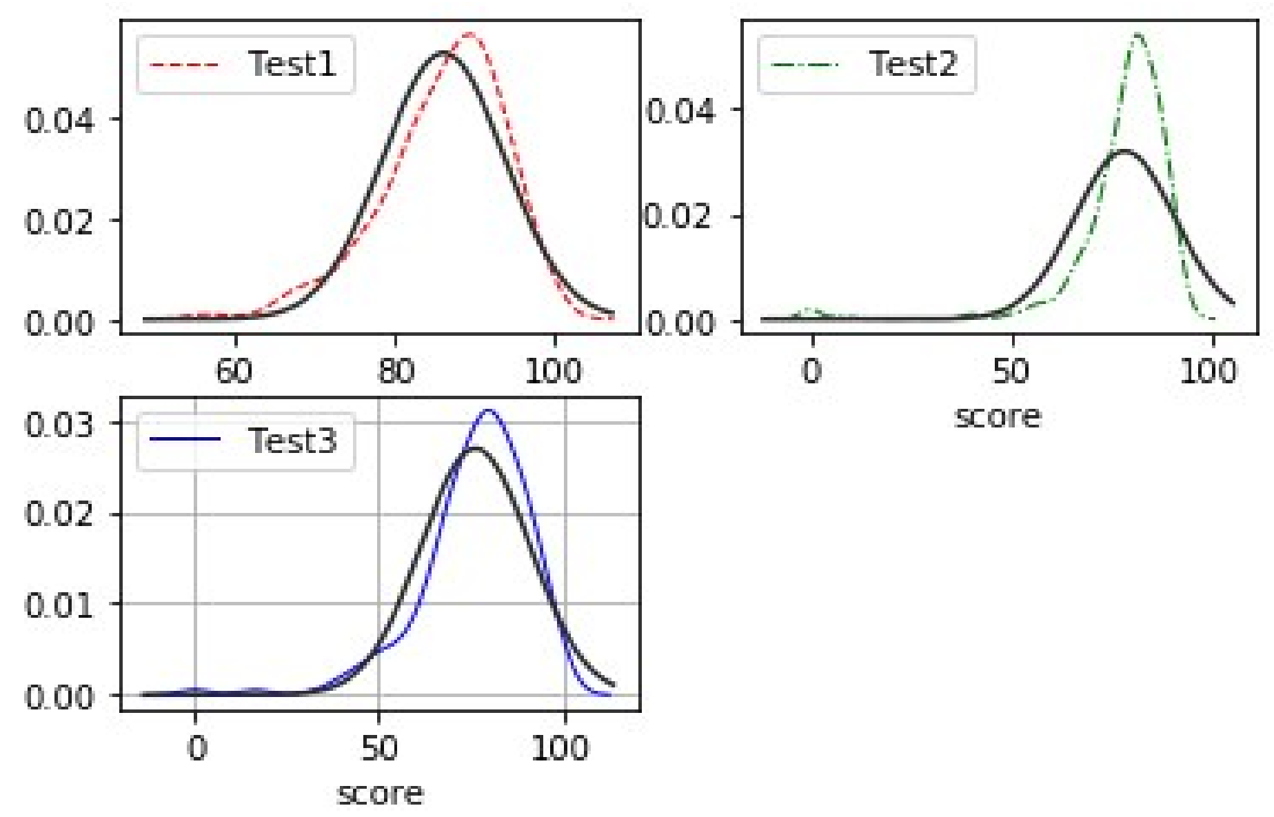
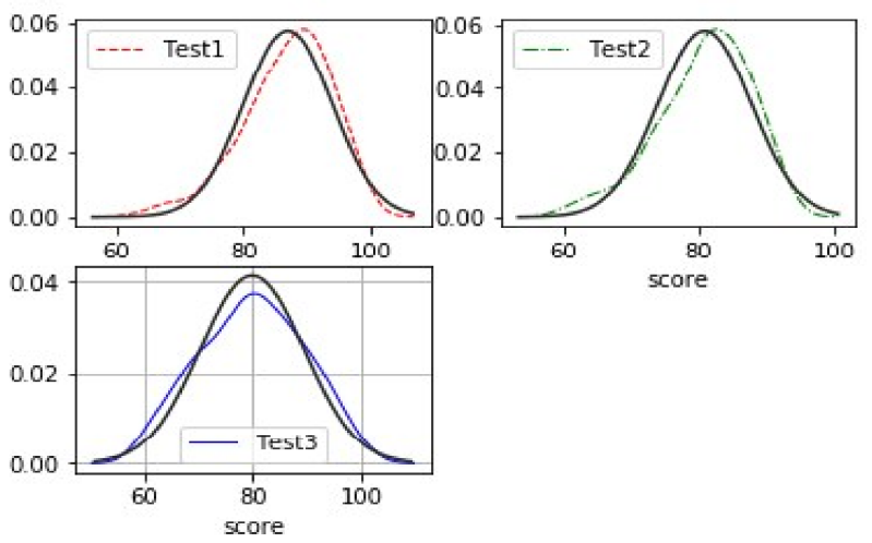
The horizontal coordinates of the graph display the distribution of the students’ scores, while the vertical coordinates display the values of the Gaussian Density Function for the score distribution.The results of the first quiz are represented by Test1, the results of the second quiz by Test 2, and the results of the third quiz by Test 3 [16].
The dataset for the experiments in this work is saved in an Excel table, and the experiments are written in Python. The results show that the sample set, which consists of 465 records, shows that the Gaussian Bayesian classifier performs well in predicting students’ grades. Table 5 displays the experimental results. Of these, 348 records make up the training data, while 117 sample records make up the prediction data. The classification accuracy of these records is 92%.
| Precision | Recall | F1-score | Support | |
|---|---|---|---|---|
| -1 | 0.85 | 0.81 | 0.88 | 10 |
| 1 | 0.85 | 1.00 | 0.94 | 22 |
| 2 | 0.95 | 0.93 | 0.95 | 25 |
| 3 | 0.95 | 0.85 | 0.92 | 35 |
| 4 | 0.94 | 0.95 | 0.96 | 118 |
| Macroavg | 0.94 | 0.90 | 0.92 | 116 |
| Weighted avg | 0.94 | 0.95 | 0.92 | 117 |
The sample set consists of 408 records after excluding all test scores lower than 60. Table 6 displays the experimental results. Of these, 306 records make up the training data, while 102 sample records make up the prediction data. The classification accuracy of these records is 96%.
| Precision | Recall | F1-score | Support | |
|---|---|---|---|---|
| 1 | 0.95 | 1.00 | 0.98 | 17 |
| 2 | 0.98 | 0.95 | 0.94 | 26 |
| 3 | 0.96 | 1.00 | 0.95 | 28 |
| 4 | 1.00 | 0.85 | 0.92 | 34 |
| Macroavg | 0.95 | 0.96 | 0.92 | 103 |
| Weighted avg | 0.95 | 0.96 | 0.94 | 102 |
Classification using the Gaussian process model is a type of generative model; these models attempt to characterise the joint distribution of \(x\) and \(y\) by modelling the posterior probability. The combined probability distribution serves as the estimate \(P\left( x \right),y\). Support vector machine classification algorithms fall under the discriminative model; however, a basic machine learning problem typically consists of two parts: input and output. For example, in the discriminative model, the conditional probability distribution \(P(y\mid x)\) is estimated and the optimal classification surface between various classes is sought after for classification.
To achieve strong statistical regularity with a limited statistical sample size, one useful classification approach is Support Vector Machine (SVM). As shown in Table 7 that different kernel functions must be selected for testing depending on whether the data are linearly separable or not, depending on the particular situation. Because the Support Vector Machine technique does not emphasise the feature dataset’s normal distributability, it is not required to reject grades below 60 in order to ensure that the data have normally distributed features. Furthermore, based on the preprocessing of the data samples grade labelling, a linear kernel function may be selected for the test; the test results show that the classification accuracy was 99%.
| Precision | Recall | F1-score | Support | |
|---|---|---|---|---|
| -1 | 0.90 | 0.96 | 0.96 | 11 |
| 1 | 0.95 | 0.97 | 0.96 | 23 |
| 2 | 0.94 | 0.94 | 0.93 | 25 |
| 3 | 0.99 | 0.98 | 0.98 | 36 |
| 4 | 0.98 | 0.96 | 0.93 | 27 |
| Macroavg | 0.98 | 0.95 | 0.99 | 116 |
| Weighted avg | 0.96 | 0.98 | 0.96 | 117 |
Taking into account that the Bayesian strategy eliminates both the overfitting issue and the subjective bias associated with relying solely on sample information by mixing a priori and a posteriori probability. This approach, together with the supposition that college English grades of students may satisfy a normal distribution, is coupled in this study to predict students’ grades effectively using the Gaussian process model classification. According to the test results, the prediction impact of the algorithm improves with sample data that is closer to the normal distribution; nevertheless, this effect is not as strong as the support vector machine algorithm’s classification effect. While other articles have also highlighted the differences in the classification effect between the standard Bayesian algorithm and the support vector machine algorithm, they have not provided a thorough demonstration of the underlying causes of these differences, which the next research work on this paper will tackle and centre around.
This work supported by Ministry of Education industry-university cooperative education project (A practical research on English teaching reform of double first-class construction in colleges and universities under the background of industry-university cooperation and collaborative education: 220901212275632); Shanxi Provincial Department of Culture and Tourism, 2022 Art Science Planning project in Shanxi Province (Research on aesthetic value and protection of folk rap art in Lyuliang: 22BB022).
The author declares no conflict of interests.