
A Hadamard matrix is an \(n \times n\) matrix \(H_n \in {\{\pm 1\}}^{n\times n}\) that satisfies \(H_n{H^{T}_n} = n{I_{n}}\). In 1896, Hadamard showed that every matrix \(M \in {\{\pm 1\}}^{n\times n}\) satisfied the inequality det\(|(M)| \leq n^{n/2}\), and any \(M \in {\{\pm 1\}}^{n\times n}\) that met this upper bound was Hadamard. It follows from this definition that if a matrix is Hadamard, the inner product of any two rows (or columns) \(\mathbf{r_{i}},\mathbf{r_{j}}\) satisfies \(\mathbf{r_i} \cdot \mathbf{r_j} = 0\) if and only if \(i\neq j\). It is straightforward to show the following (see [1] for details).
Proposition 1. If \(H_n\) is a Hadamard matrix of order \(n\), then:
\(n\) must be \(1,2\) or \(4k\), where \(k \in \mathbb{N}\).
Both \(-H_n\) and \(H_{n}^{T}\) are also Hadamard.
Permuting rows and/or columns leaves \(H_n\) Hadamard.
Multiplying any row or column by \(-1\) leaves \(H_n\) Hadamard.
Two Hadamard matrices \(H_{n}\) and \(H_{n}'\) of order \(n\) are equivalent, denoted \(H_{n} \sim H_{n}'\), if \(H_{n}'\) can be obtained from \(H_{n}\) by permuting rows, permuting columns, and negating rows and columns. It is easy to show that \(\sim\) generates an equivalence relation on the set of all Hadamard matrices of a given order. A resulting equivalence class is often represented by a normalized Hadamard matrix – that is, a Hadamard matrix with all \(1\)’s in the initial row and column.
In 1896, Scarpis [2] published an unusual technique for constructing Hadamard matrices of order \(p(p+1)\), where \(p\) is a prime with \(p \equiv 3 (\) \(4)\). His approach appears somewhat ad hoc and is awkward to implement, which may be one of the reasons that his method, while sound, has not received the same attention as the more straightforward approaches of, among others, Sylvester and Paley. To date, the only other direct use of the method of Scarpis appears in [3], where Djokovic shows the Scarpis construction also generates Hadamard matrices of order \(q(q+1)\) where \(q\) is any prime power with \(q \equiv 3 (\) \(4)\). In this article, we will show that the method of Scarpis can be generalized to construct complex Hadamard matrices.
Before presenting both the Scarpis construction and our generalization to CHMs, some historical clarification is needed.
Williamson [4] mentions, but does not use, the method of Scarpis in his Hadamard constructions; he simply compares the known orders of Hadamard matrices that result from the methods of Paley and Scarpis to show that his results generate new orders of Hadamard matrices.
Mukhopadhyay [5] identifies some orders of Williamson Hadamard matrices that exist, but his approach is based on the Paley construction, and these orders only coincide with the orders of Hadamard matrices outlined by Scarpis in their base case. In addition, Seberry [6] notes that the Mukhopadhyay construction yields no new Hadamard matrices of orders \(< 40,000\). Moreover, the results of Mukhopadhyay are based on the existence of \(L\)-matrices, but no examples of \(L\)-matrices are provided. On the other hand, both the original Scarpis method and our CHM-based generalization are constructive. Thus, our main result, that the Scarpis construction can be generalized to CHMs, is distinct from the work in [5] and [6].
Here is the original construction of Scarpis.
Proposition 2. Let \(H_n\) be a normalized Hadamard matrix of order \(n=p+1\), where \(p \equiv 3(\) \(4)\) is prime.
Arrange the columns of \(H_n\) so that row \(2\) consists of alternating \(1\)’s and \(-1\)’s.
Construct \(H^2\), the matrix formed by deleting the \(2^{nd}\) row of \(H_n\).
Construct the \(p \times p(p+1)\) matrix \(M' = H^2\otimes \mathbf{J}\) (\(\mathbf{J}\) is the \(1 \times p\) vector of 1’s).
Construct \(C\), the core of \(-H_n\), whose rows are denoted \(\mathbf{a_0} , \mathbf{a_1},…, \mathbf{a_{p-1}}\).
For each \(0 \leq r \leq p-1\), construct the \(p \times p(p+1)\) block matrix \(M_r\) defined by \[M_r = \begin{bmatrix} \mathbf{a_r} & -\mathbf{a_0} & \mathbf{a_r} & -\mathbf{a_{2r}} & \ldots & \mathbf{a_{(p-2)r}} & -\mathbf{a_{(p-1)r}}\\ \mathbf{a_r} & -\mathbf{a_1} & \mathbf{a_{r+1}} & -\mathbf{a_{2r+1}} & \ldots & \mathbf{a_{(p-2)r+1}} & -\mathbf{a_{(p-1)r+1}} \\ \vdots & \vdots & \vdots & \vdots & \ddots & \vdots & \vdots \\ \mathbf{a_r} & -\mathbf{a_{p-1}} & \mathbf{a_{r+(p-1)}} & -\mathbf{a_{2r+(p-1)}} & \ldots & \mathbf{a_{(p-2)r+(p-1)}} & -\mathbf{a_{(p-1)r+(p-1)}} \\ \end{bmatrix}.\] Then the block matrix \(M\) below is a Hadamard matrix of order \(p(p+1)\): \[M=\begin{bmatrix} M' \text{ } M_0 \text{ } M_1 \text{ } \ldots \text{ } M_{p-1} \end{bmatrix}^{T}.\]
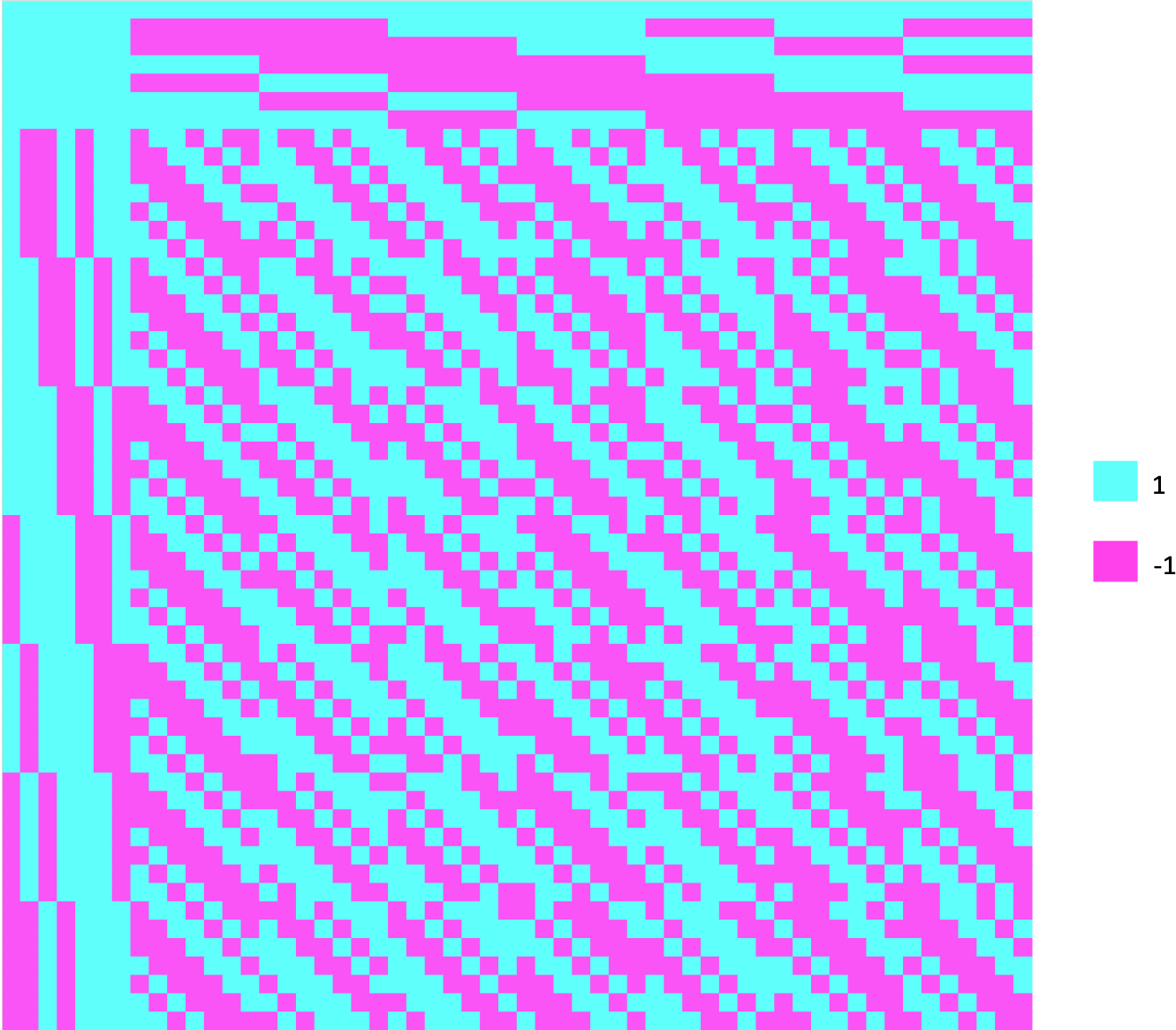
Figure 1 is for a color-coded example of a Scarpis Hadamard matrix, constructed using the prime \(p=7\). As mentioned in [7], the Scarpis construction, used in conjunction with the methods of Paley and Sylvester, results in new orders of Hadamard matrices.
Given any primitive \(m^{th}\) root of unity \(\omega\), a complex Hadamard matrix of order \(n\), or CHM, often called a Butson-type Hadamard matrix, is a matrix \(H_n \in {\{\omega^i | 1\leq i \leq m \}}^{n\times n}\) that satisfies \(H_n H^{*}_n = n{I_{n}}\), where \(H^{*}_n\) denotes the complex conjugate transpose of \(H_n\). Unlike the real case, there exists a CHM of every order. The following are well-known results, see [1] for details.
Proposition 3. If \(H_n\) is a CHM, then
Permuting rows and/or columns of \(H_n\) yields a CHM.
Each of \(-H_n\), \(H_n^{T}\) and \(H_n^{*}\) is also a CHM.
Multiplying a row/column of \(H_n\) by any \(m^{th}\) root of unity yields a CHM.
If \(H_n\) is normalized, each noninitial row or column sums to \(0\).
Two CHMs \(H_{n}\) and \(H_{n}'\) are equivalent, denoted \(H_{n} \sim H_{n}'\), if \(H_{n}'\) can be obtained from a permutation of the rows or columns of \(H_{n}\), allowing any row or column to be multiplied by any \(m^{th}\) root of unity.
The Scarpis construction generalizes directly into a CHM, but with two important differences: the construction can be based on any prime \(p\), and any row may be deleted from \(H_n\), the initial normalized CHM. Here is our generalization.
Theorem 1. Let \(p\) be any prime, and let \(H_n\) be a normalized CHM of order \(n = p+1\). Now define the following
\(\mathbf{\mathbf{ r_k}}\), the \(k^{th}\) row of \(H_n\), whose entries are \(x_1, x_2, … ,x_n\).
\(H^k\), the \(p \times n\) matrix resulting from removing \(\mathbf{ r_k}\) from \(H_n\).
\(M'\), the order \(p(p+1)\) matrix defined via \(M' = H^k\otimes \mathbf{J}\).
\(C\), the core of \(-H_n\), whose rows are in order \(\mathbf{a_0} , \mathbf{a_1},…, \mathbf{a_{p-1}}\).
For each \(0 \leq r \leq p-1\), construct the \(p \times p(p+1)\) matrix \(M_r\), defined in block form as \[\begin{bmatrix} x_1 \mathbf{a_r} & x_2 \mathbf{a_0} & x_3 \mathbf{a_r} & x_4 \mathbf{a_{2r}} & \ldots & x_{n-1} \mathbf{a_{(p-2)r}} & x_{n} \mathbf{a_{(p-1)r}}\\ x_1 \mathbf{a_r} & x_2 \mathbf{a_1} & x_3\mathbf{a_{r+1}} & x_4 \mathbf{a_{2r+1}} & \ldots & x_{n-1} \mathbf{a_{(p-2)r+1}} & x_{n} \mathbf{a_{(p-1)r+1}} \\ \vdots & \vdots & \vdots & \vdots & \ddots & \vdots & \vdots \\ x_1 \mathbf{a_r} & x_2 \mathbf{a_{p-1}} & x_3 \mathbf{a_{r+(p-1)}} & x_4 \mathbf{a_{2r+(p-1)}} & \ldots & x_{n-1} \mathbf{a_{(p-2)r+(p-1)}} & x_{n} \mathbf{a_{(p-1)r+(p-1)}} \\ \end{bmatrix}.\] Then the block matrix \(M\) below is a CHM of order \(p(p+1)\): \[M=\begin{bmatrix} M' \text{ } M_0 \text{ } M_1 \text{ } \ldots \text{ } M_{p-1} \end{bmatrix}^{T}.\]
We now give an example, using \(p=5\), of this generalized Scarpis construction.
Example 1. Let \(p = 5\). Note that \(H_n = \begin{bmatrix} 1 & 1 & 1 & 1 & 1 & 1 \\ 1 & -1 & i & -i & -i & i \\ 1 & i & -1 & i & -i & -i \\ 1 & -i & i & -1 & i & -i \\ 1 & -i & -i & i & -1 & i \\ 1 & i & -i & -i & i & -1 \end{bmatrix}\) is a normalized quaternary CHM. Deleting the third row of \(H_n\) gives us \[H^3 =\begin{bmatrix} 1 & 1 & 1 & 1 & 1 & 1 \\ 1 & -1 & i & -i & -i & i \\ 1 & -i & i & -1 & i & -i \\ 1 & -i & -i & i & -1 & i \\ 1 & i & -i & -i & i & -1 \end{bmatrix}.\] Note that \(\mathbf{r_3} = \begin{bmatrix} 1 & i & -1 & i & -i & -i \end{bmatrix}.\) Also note that \[M' = \begin{bmatrix} 1 & 1 & 1 & 1 & 1 & 1 \\ 1 & -1 & i & -i & -i & i \\ 1 & -i & i & -1 & i & -i \\ 1 & -i & -i & i & -1 & i \\ 1 & i & -i & -i & i & -1 \end{bmatrix} \otimes \begin{bmatrix} 1 & 1 & 1 & 1 & 1 \end{bmatrix},\] which simplifies to \[\left[\begin{array}{cccccccccccccccccccccccccccccc} 1 & 1 & 1 & 1 & 1 & 1 & 1 & 1 & 1 & 1 & 1 & 1 & 1 & 1 & 1 & 1 & 1 & 1 & 1 & 1 & 1 & 1 & 1 & 1 & 1 & 1 & 1 & 1 & 1 & 1 \\ 1 & 1 & 1 & 1 & 1 & -1 & -1 & -1 & -1 & -1 & i & i & i & i & i & -i & -i & -i & -i & -i & -i & -i & -i & -i & -i & i & i & i & i & i \\ 1 & 1 & 1 & 1 & 1 & -i & -i & -i & -i & -i & i & i & i & i & i & -1 & -1 & -1 & -1 & -1 & i & i & i & i & i & -i & -i & -i & -i & -i \\ 1 & 1 & 1 & 1 & 1 & -i & -i & -i & -i & -i & -i & -i& -i & -i & -i & i & i & i & i & i & -1 & -1 & -1 & -1 & -1 & i & i & i & i & i \\ 1 & 1 & 1 & 1 & 1 & i & i & i & i & i & -i & -i& -i & -i & -i & -i & -i & -i & -i & -i & i & i & i & i & i & -1 & -1 & -1 & -1 & -1 \end{array}\right].\] The core of \(-H\) is \(C = \begin{bmatrix} 1 & -i & i & i & -i \\ -i & 1 & -i & i & i \\ i & -i & 1 & -i & i \\ i & i & -i & 1 & -i \\ -i & i & i & -i & 1 \end{bmatrix}\). We then label the rows of \(C\) as \[\begin{aligned} &\mathbf{a_0} = \begin{bmatrix} 1 & -i & i & i & -i \end{bmatrix}, \\ &\mathbf{a_1} = \begin{bmatrix} -i & 1 & -i & i & i \end{bmatrix}, \\ &\mathbf{a_2} = \begin{bmatrix} i & -i & 1 & -i & i \end{bmatrix}, \\ &\mathbf{a_3} = \begin{bmatrix} i & i & -i & 1 & -i \end{bmatrix}, \\ &\mathbf{a_4} = \begin{bmatrix} -i & i & i & -i & 1 \end{bmatrix}. \end{aligned}\] Next, we construct each block matrix \(M_r\). For brevity, we will only construct \(M_0\) \[M_0 = \begin{bmatrix} \mathbf{a_0} & i \mathbf{a_0} & -1 \mathbf{a_0} & i \mathbf{a_0} & -i \mathbf{a_0} & -i \mathbf{a_0} \\ \mathbf{a_0} & i \mathbf{a_1} & -1 \mathbf{a_1} & i \mathbf{a_1} & -i \mathbf{a_1} & -i \mathbf{a_1} \\ \mathbf{a_0} & i \mathbf{a_2} & -1 \mathbf{a_2} & i \mathbf{a_2} & -i \mathbf{a_2} & -i \mathbf{a_2} \\ \mathbf{a_0} & i \mathbf{a_3} & -1 \mathbf{a_3} & i \mathbf{a_3} & -i \mathbf{a_3} & -i \mathbf{a_3} \\ \mathbf{a_0} & i \mathbf{a_4} & -1 \mathbf{a_4} & i \mathbf{a_4} & -i \mathbf{a_4} & -i \mathbf{a_4} \end{bmatrix},\] where \(M_0\) is a \(5 \times 30\) matrix and each \(\mathbf{a_i}\) block is of size \(1 \times 5\). Note, for instance, that \[i \mathbf{a_2} = i \begin{bmatrix} i & -i & 1 & -i & i \end{bmatrix} = \begin{bmatrix} -1 & 1 & i & 1 & -1 \end{bmatrix}.\] Finally, we construct \(M\):
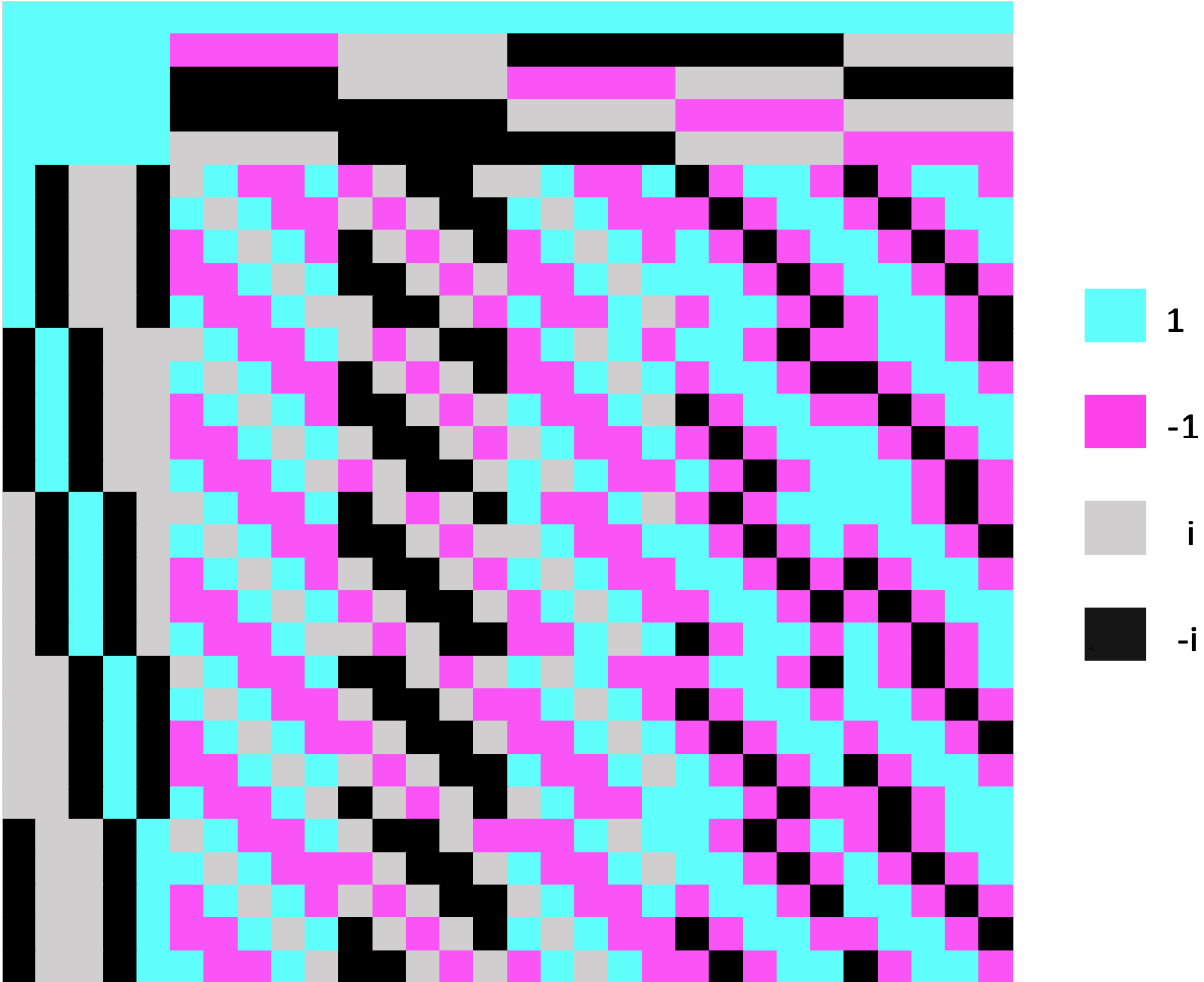
\(M = \begin{bmatrix} M' \text{ } M_0 \text{ } M_1 \text{ } M_2 \text{ } M_3 \text{ } M_4 \end{bmatrix}^{T}\).
For a color-coded visual representation of \(M\), see Figure 2.
Proof. Given any prime \(p\), to prove that the matrix \(M\) in the statement of Theorem 1 yields a CHM, we will show that every pair of distinct rows of \(M\) is mutually orthogonal. To begin, note that the orthogonality of pairs of distinct rows of \(M' = H^k\otimes \mathbf{J}\) follows directly from the orthogonality of the rows of \(H_n\).
Secondly, we must show pairwise orthogonality of distinct rows within each \(M_r\). To this end, we fix \(r\) and compare two rows of \(M_r\). Recall that the row blocks that build these rows are generated from the rows of \(C\). Note that one pair of row blocks in one column are identical, whereas the remaining pairs of row blocks in all other columns are distinct. It is clear that this is the case for any prime \(p\): any two rows of \(M_r\) will, by definition, include one pair of row blocks of \(C\) that are identical, while the remaining \(n = p+1\) pairs of row blocks of \(C\) will be distinct.
Let \(\mathbf{a_t} = \begin{bmatrix} \mathbf{a_{t,1}} & \mathbf{a_{t,2}} & … & \mathbf{a_{t,p}}\end{bmatrix}\) be any row of \(-C\). Because the entries in \(\mathbf{a_t}\) are roots of unity, it follows that \(\mathbf{a_t} \cdot \overline{\mathbf{a_t}} = p\), since \(\mathbf{a_t}\) is a vector of length \(p\). Also note that because each \(\mathbf{a_n}\) is a row of the core of a normalized matrix with all distinct rows pairwise orthogonal, each of their inner products are \(0\). Since \(C\) is the core of \(-H_n\), it follows that for distinct \(s\) and \(t\), \(\mathbf{a_t} \cdot \overline{\mathbf{a_s}} = -1\).
Thirdly, we must show that each row of \(M'\) is orthogonal to each row of \(M_r\). Consider the inner product of the \(b^{th}\) row of \(M'\) and an arbitrary row of \(M_r\) for some \(r\), which involves products of the form \(y_i\mathbf{J} \cdot \overline{x_i\mathbf{a_t}},\) where \(x_i\) is an arbitrary entry in \(\mathbf{ r_k}\) and \(y_i\) is an arbitrary entry in a row of \(H_n\) distinct from \(\mathbf{ r_k}\) and \(\mathbf{J}\) is the \(1 \times p\) vector of all \(1\)’s. Since \(C\) is the core of \(-H_n\), the elements in each row of \(C\) sum to \(1\). Thus, \[\begin{aligned} y_i\mathbf{J}\cdot\overline{x_i \mathbf{a_t}} &= (y_i \overline{x_i})\mathbf{J}\cdot \overline{\mathbf{a_t}}\\ & =y_i \overline{x_i} (\overline{\mathbf{a_{t,1}}}+\overline{\mathbf{a_{t,2}}}+…+\overline{\mathbf{a_{t,p}}})\\ & =y_i \overline{x_i} (1) \\ & =y_i \overline{x_i}. \end{aligned}\] It then follows that inner product of the entire \(b^{th}\) row of \(M'\) and an arbitrary row of \(M_r\) for some \(r\) is \[\begin{aligned} & y_{1}\overline{x_{1}} + y_{2}\overline{x_{2}} + … + y_{n}\overline{x_{n}} = 0, \end{aligned}\] since this is the complex inner product of two rows of the original complex Hadamard matrix \(H_n\).
Lastly, we must show that for any \(r \neq s\), the rows of \(M_r\) and \(M_s\) are pairwise orthogonal. Let \(\mathbf{u}\) denote the \(\alpha^{th}\) row of \(M_r\), and let \(\mathbf{v}\) denote the \(\beta^{th}\) row of \(M_s\), where \(0 \leq \alpha, \beta \leq p-1\). That is,
\(\mathbf{u} = \begin{bmatrix} x_1\mathbf{a_{r}} & x_2\mathbf{a_{\pmb{\alpha}}} & x_3\mathbf{a_{(r+\pmb{\alpha})}} & … & x_n\mathbf{a_{(p-1)r+\pmb{\alpha})}} \end{bmatrix}\),
\(\mathbf{v} =\begin{bmatrix} x_1\mathbf{a_{s}} & x_2\mathbf{a_{\pmb{\beta}}} & x_3\mathbf{a_{(s+\pmb{\beta})}} & … & x_n\mathbf{a_{(p-1)s+\pmb{\beta})}} \end{bmatrix}\).
Note that the inner product of \(\mathbf{u}\) and \(\mathbf{v}\) satisfies
\(\mathbf{u} \cdot \overline{\mathbf{v}} = \mathbf{\mathbf{a_r}} \cdot \overline{\mathbf{a_s}} + {{\sum}}_{i = 0}^{p-1} \mathbf{a_{ir+\pmb{\alpha}}}\cdot \overline{\mathbf{a_{is+\pmb{\beta}}}}\),
where the subscripts are reduced modulo \(p\). This sum will have \(p\) pairs of distinct vector products, and exactly one such pair wherein the two vectors are the same. The matching pair occurs at the unique value of \(i\) that satisfies \(i(r-s) \equiv \beta-\alpha (\text{mod} \text{ }p)\). It then follows that \(\mathbf{u} \cdot \mathbf{v} = 0\). Therefore, \(M\) is a CHM. ◻
As Djokovic shows in [3], the classic Scarpis construction can be modified to generate Hadamard matrices of order \(q(q+1)\) where \(q\) is any prime power and \(q \equiv 3 (\) \(4)\). This restriction on \(q\) is unnecessary in CHM constructions as CHMs can exist of order \(p+1\) where \(p \equiv 1 (\) \(4)\).
Let \(\mathcal{CH}_{n}\) be the set of complex Hadamard matrices of a given order \(n\) and let \(\mathbb{F}_q\) denote the unique finite field of order \(q\). Given a bijection \[\alpha: \{0,1,2,3… ,q-1\} \rightarrow \mathbb{F}_{q},\] where \(q\) is an odd prime power, the algorithm described in Theorem 1 yields a map \[\Phi_{q,\alpha}: \mathcal{CH}_{q} \rightarrow \mathcal{CH}_{q(q+1)},\] in which the multiplication occurs in \(\mathbb{F}_q\) – specifically, \(\mathbf{a_{i}} = \mathbf{a_{\alpha(i)}}\) and \(\mathbf{a_{j\cdot r+k}} = \mathbf{a_{\alpha(j)\cdot\alpha(r)+\alpha(k)}}\). These observations lead to the following generalization of Theorem 1.
Corollary 1. Let \(H\) be a CHM of order \(q+1\) where \(q\) is an odd prime power. Then there exists a CHM of order \(q(q+1)\).
It is worth noting that the pattern of + and – signs in the \(2^{nd}\) row removed from \(H_n\) in the classic Scarpis construction is identical to the pattern of + and – signs attached to the columns of each block matrix \(M_r\). This is not a coincidence. In fact, just as in our generalized Scarpis construction, any row could have been removed from \(H_n\) in the classic Scarpis construction. In a similar vein, Scarpis unnecessarily negated the core of \(H_n\) in his construction, whereas Djokovic does not do so in his generalization to prime powers. In what follows, we let \(H(k;)\) denote a given matrix \(H\) with the \(k^{th}\) row removed.
Corollary 2. In the classic Scarpis construction, given any \(1 \leq k \leq p+1\), let \(x_1, x_2, … x_{n}\) denote the entries of the removed \(k^{th}\) row, and let \(H(k;)\) denote the remaining matrix. The resulting block matrices \(M_r\) for \(0 \leq r \leq p-1\) that comprise the resulting Scarpis Hadamard matrix are given by \[\begin{bmatrix} x_1 \mathbf{a_r} & x_2 \mathbf{a_0} & x_3 \mathbf{a_r} & x_4 \mathbf{a_{2r}} & \ldots & x_{n-1} \mathbf{a_{(p-2)r}} & x_{n} \mathbf{a_{(p-1)r}}\\ x_1 \mathbf{a_r} & x_2 \mathbf{a_1} & x_3\mathbf{a_{r+1}} & x_4 \mathbf{a_{2r+1}} & \ldots & x_{n-1} \mathbf{a_{(p-2)r+1}} & x_{n} \mathbf{a_{(p-1)r+1}} \\ \vdots & \vdots & \vdots & \vdots & \ddots & \vdots & \vdots \\ x_1 \mathbf{a_r} & x_2 \mathbf{a_{p-1}} & x_3 \mathbf{a_{r+(p-1)}} & x_4 \mathbf{a_{2r+(p-1)}} & \ldots & x_{n-1} \mathbf{a_{(p-2)r+(p-1)}} & x_{n} \mathbf{a_{(p-1)r+(p-1)}} \\ \end{bmatrix}.\]
It appears that each choice of a \(k^{th}\) deleted row of the original CHM results in the larger Scarpis-constructed CHM. The different choices of \(k\) generally result in different equivalence classes; however, this is not always true and it is unclear under what circumstances this does not hold.
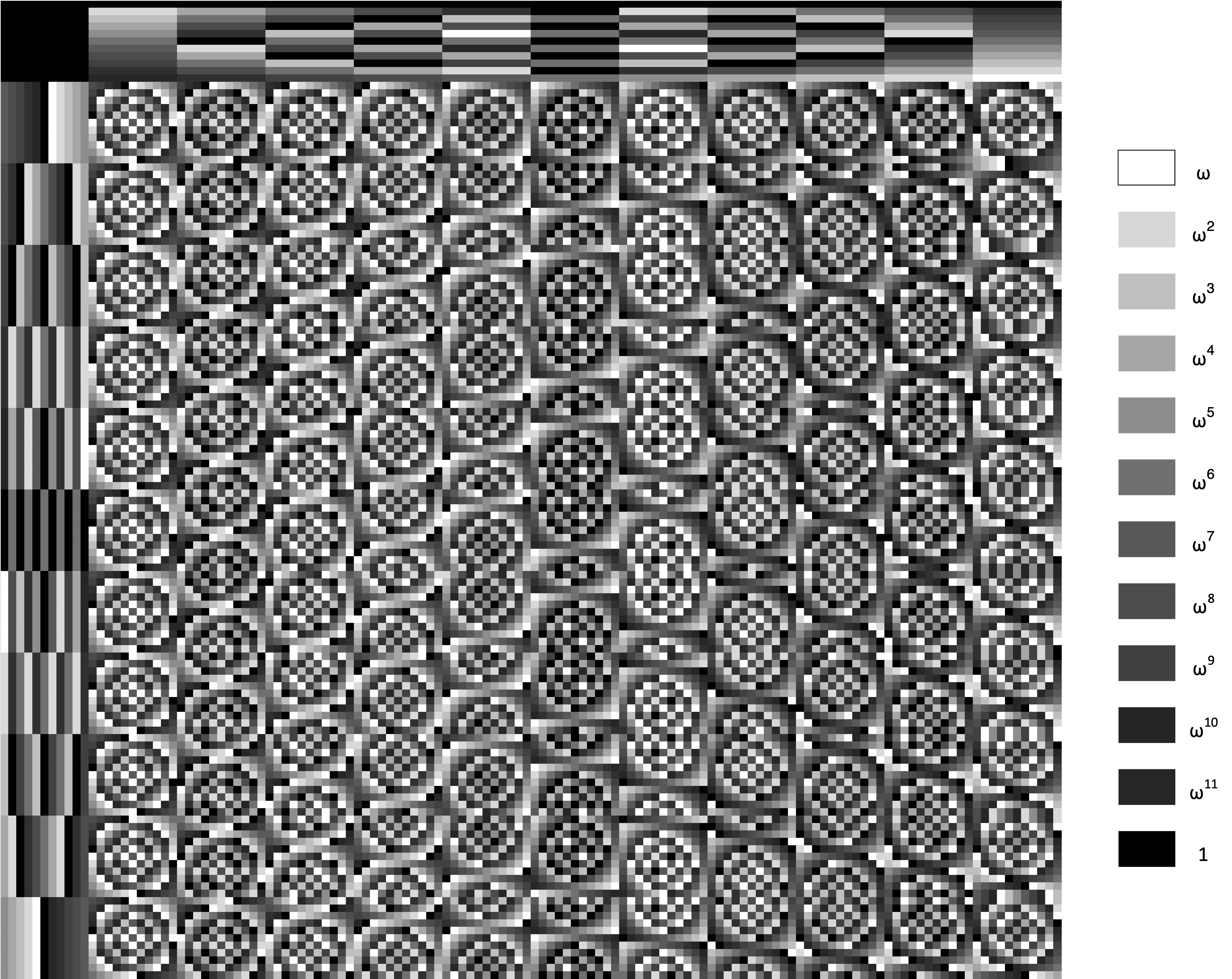
We note that our Scarpis-inspired CHM construction can be employed in more general contexts, such as using Vandermonde matrices generated using a primitive complex \(p+1^{st}\) root of unity as the initial seed matrix. See Figure 3 for an example.
\(\textbf{Open Problem}\) In our generalized complex Scarpis construction, determine conditions under which the choices of a \(k^{th}\) deleted row of a given CHM results in larger Scarpis-constructed CHMs belonging to different equivalence classes.
We thank the anonymous referees for their helpful comments.