
Agriculturee is an important driving force for national development, and an important manifestation of the country’s comprehensive national strength. With the rapid economic and social development and the prosperity of the market [1]. Agricultural economic management emerged as a new management model. The connotation and extension of agricultural economic management are relatively broad, involving various links such as agricultural production, product processing, sales, and circulation. The author believes that agricultural economic management refers to making full use of various factors such as financial resources, material resources, human resources, and natural resources according to the laws of natural economy, continuously improving the initiative of farmers and rural areas, comprehensively improving the quality and efficiency of agricultural economy, and finally realizing agricultural economy. sustainable and healthy development [2]. However, the development of everything has two sides, and the management of agricultural economy is no exception. It also has some challenges, which seriously affect and restrict the development of rural economy. Through investigation, the author found that some thorny problems in the process of rural economic development can be better solved by optimizing agricultural economic management measures. Therefore, it is very important to analyze the role of agricultural economic management in promoting the development of rural economy, and it is of great significance to promote the sustainable development of rural economy [3].
Under the current circumstances, the effective management of agricultural economy plays a very important role in the development of rural economy and is closely related to the level and quality of rural economic development to a certain extent. Strengthening the management mode of agricultural economy can make agricultural economy more executable and scientific. To a certain extent, it can also make full use of the existing resources in rural areas, Adapt to local conditions. Through the scientific management of the agricultural economy, the rural economic development has a scientific and efficient institutional mechanism, which can fundamentally improve the standardization and effectiveness of the rural economy and add a steady stream of vitality to the rural economic development. and vitality [4]. In addition, through the allocation of scientific means and the use of policy incentives, farmers’ enthusiasm for production can be greatly improved, and farmers’ worries can be completely solved. With the continuous social and economic breakthroughs and progress, the rural economic development has ushered in a new development opportunity, which is both an opportunity and a challenge for the rural economy. At the same time, various new technologies emerge in an endless stream, and the application of these emerging technologies can provide a continuous boost to the economic development of rural areas to a certain extent.
Although the rural economy has ushered in a new development direction, it has also brought some problems and challenges. The emergence of these problems has put forward higher requirements and expectations for managers. Under such circumstances, the purposeful optimization of the management plan of the rural economy can turn the disadvantageous conditions into favorable conditions to a certain extent, provide more plans for rural economic development, and truly benefit more farmers [5].
The vector autoregressive model \(VAR\) was proposed by Christopher Sims in 1980. The \(VAR\) model uses each endogenous variable in the system as a function of the lagged values of all endogenous variables in the system to construct the model. Because there is no need to presuppose the existence of a theoretical economic relationship between various economic variables, it is widely used. \(VAR_{\left( p \right)}\) model expression with variables:
\[\label{e1}\tag{1} Y_t=\mu+A_1 Y_{t-1}+\ldots+A_p Y_{t+p}+\xi(t=1,2, \ldots, T),\] where \({y_t}\) is the \(t\) dimensional endogenous variable vector, \(p\) is the lag order number, \(T\) is the number of samples,\({A_1},…,{A_P}\) is an\(n \times n\)dimensional coefficient matrix, \(\zeta t – {N_{(0,\sum )}}\)is \(k\)dimensional random error vector. Any \(MA\left( \infty \right)\) model can be represented as an infinite-order vector process.
\[\label{e2}\tag{2} {y_{t + s}} = {U_{t + s}} + {\psi _1}{U_{t + s – 1}} + {\psi _2}{U_{t + s – 2}} + …,\]
\[\label{e3}\tag{3} {\psi _s} = \frac{{\partial {Y_{t + s}}}}{{\partial {U_t}}},\] where \({\psi _s}\) is the elements in the \(i\)th row and the \(j\)th column represent that under the condition that the other error terms remain unchanged in any period, When the error term\({u_{jt}}\) corresponding to the \(j\) variable \({y_{it}}\) is impacted by one unit in the \(t\) period, the impact on the \(i\) endogenous variable \({y_{it}}\) in the\(t + s\) period. Consider the element in row \(i\) and column \(j\) in \({\psi _s}\) as a function of lag period \(s\):
\[\label{e4}\tag{4} \frac{{\partial {y_{i,t + s}}}}{{\partial {u_{it}}}},s = 1,2,3,…n.\]
The above formula is the impulse response function (impulse-response function), the impulse response function describes the premise that other variables remain unchanged in the\(t\) period and the previous periods, \({y_{i,t + s}}\) to \({u_{j,t}}\) a shock reaction process.
The \(VAR\) model constructs a function of each endogenous variable and determining each Parameter estimation and other analyses are performed after the lag order of the endogenous variables. The process of establishing a \(VAR\) model is generally as follows: if there are \(k\) time series variables:
\[\label{e5}\tag{5} y_{1 t}, y_{2 t}, \ldots, y_{k t} y_t=\left[\begin{array}{l} y_{1 t} \\ y_{2 t} \\ \ldots \\ y_{k t} \end{array}\right],\quad t=1,2, \ldots, T.\]
Then the expression of the P order \(VAR\) model, that is,\(VAR\left( P \right)\):
\[\label{e6} {y_t} = {A_1}{y_{t + 1}} + … + {A_p}{y_{t – p}} + { \in _t} + C.\]
Among them, \({y_t}\) is the k-dimensional endogenous variable vector, p is the lag order, the number of samples is t, t is the k-dimensional disturbance variable, and C is the k-dimensional constant vector. The \(VAR\) theory requires that each time series variable entered the model is a stationary sequence. If the time series variable is not stationary, the time series variable needs to be differentiated, and a \(VAR\) model is established for the stationary sequence after the difference, and then the differentiated variables are further processed [6].
The pollution produced by industrial enterprises above designated size has created a great barrier to economic development. Therefore, the research object of this paper mainly selects industrial enterprises above designated size in my country [7]. The green growth model in this paper refers to protecting the environment through pollutant treatment in the development of enterprises and making the enterprise itself assume social responsibility to achieve a state of sustainable development. Therefore, we choose to use industrial enterprise pollution source control investment indicators to measure green growth, with letters GGM said [8, 9]. There are many indicators involved in measuring the development of an enterprise. The growth of an enterprise is the performance of the sustainable development of the enterprise. In order to more accurately represent the growth of the enterprise, this paper selects the total assets of the enterprise, the current assets of the enterprise, the fixed assets of the enterprise, the owner’s equity of the enterprise, and the main business of the enterprise [10]. Income, main business of the enterprise. There are 8 indicators of taxation, total corporate profits, and turnover of corporate current assets. The entropy method is used to aggregate 8 indicators into a corporate growth index to measure corporate growth, which is represented by the letter EGA.
First, the ADF method is used to test the unit root of green growth and enterprise growth. The results are shown in Table 1. The Prob. values after the first-order difference of the two variables are 0.0589 and 0.0994, respectively, which are both less than 0.1, that is, at the level of 10%. In a significant state, the null hypothesis (the time series is not stationary) is rejected, so the two variables are a first-order single integral sequence with a stationary relationship, which can be tested for cointegration.
| Original order test | First order test | ||||||||
| Time series | T statistic | Lag period | Prob | Conclusion | Time series | T statistic | Lag period | Prob | Conclusion |
| GGM | -1.534532 | 1 | 0.4853 | Nonstationary | D(GGM) | -3.023022 | 0 | 0.0589* | Stable |
| EGA | 0.562408 | 1 | 0.9823 | Nonstationary | D(EGA) | -2.646207 | 0 | 0.0994* | Stable |
Then use the E-G two-step method to perform the cointegration test of the variables. The results are shown in Table 2. The ADF unit root test of the residual sequence passed at the 5% significance level. The residual series of variables is stationary and the GGM. The two variables of EGA and EGA are cointegrated, indicating that the regression model of green growth and enterprise growth constructed in this paper is effective [11]. The green growth model will cause the enterprise growth to temporarily deviate from the equilibrium position in the short term, but the long-term choice of the green growth model will make the enterprise growth trend. In a balanced position, it is conducive to the sustainable development of enterprises, (see Figure 1).
| – | – | t-Statistic | Prob. |
|---|---|---|---|
| Augmented Dickey-Fuller test statistic | – | -3.880187 | 0.0166 |
| Test critical values | 1%lvel | -4.200055 | – |
| – | 5%lvel | -3.175354 | – |
| – | 10%lvel | -2.728986 |
Generally, the form of variables entering a model is required to be a stationary series. If non-stationary variables enter the model, it will lead to model instability and false analysis results[12]. In this paper, the stationarity of time series variables is tested before the actual modeling, and the unit root test is performed on each variable to ensure that each variable entering the model is a stationary variable. The test results using EViews are shown in Table 3.
| Variable name | ADF statistics | 5% critical value | 10% critical value | Conclusion |
|---|---|---|---|---|
| Income | -1.285078 | -4.008156 | -3.460792 | Nonstationary |
| Basis | -1.420423 | -4.008156 | -3.460792 | Nonstationary |
| D(Income) | -3.603181 | -3.259806 | -2.771128 | Stable |
| D(Internet) | -2.493008 | -1.988197 | -1.600142 | Stable |
| D(basis) | 2.781062 | -3.259806 | -2.771128 | Stable |
It can be seen from Table 3. that although the income, Internet, and basis sequences are all non-stationary, they are all stationary after the first-order difference. Therefore, the data of residents’ income, agricultural economy consumption finance, and residents’ basic subsistence consumption can be modeled after a first-order difference, and a conclusion can be drawn[13]. The data sequence after the first-order difference represents the change of the original data sequence, that is, D(income) represents the annual increase of residents’ income, D(internet) represents the annual growth of the agricultural economy’s consumption financial scale, and D(basis) represents the annual growth of the residents’ basic subsistence consumption expenditure. Therefore, this paper studies the dynamic relationship between the growth of various variables.
Before building a VAR model, it is used to determine the lag order of the VAR model. The test results are shown in Table 4.
| Lag | LogL | LR | FPE | AIC | SC | HQ |
|---|---|---|---|---|---|---|
| 0 | 13.00374 | NA | 2.18e-06 | -2.223056 | -2.157314 | -2.364928 |
| 1 | 33.07843 | 22.30519 | 2.27e-07 | -4.684094 | -4.421128 | -5.251574 |
As shown in Table 4, according to the test of LR, FPE, AIC, SC, HQ and other criteria, considering the degree of freedom of the model, the lag order of this VAR model is set to 1 in this paper.
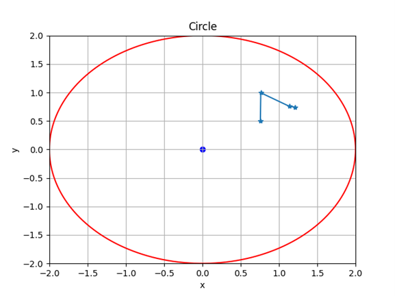
Among them, the unit circle test needs to be performed on the VAR model, as shown in Figure 2.
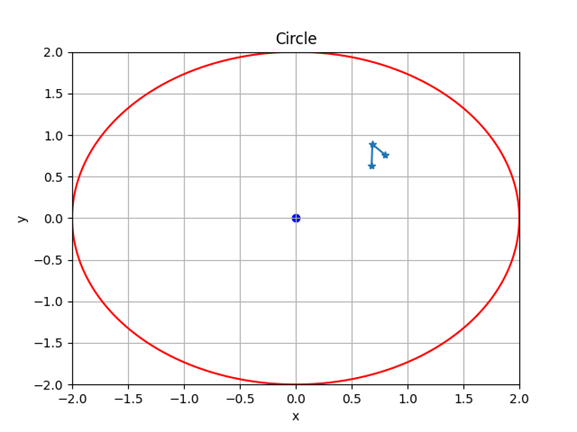
It can be seen from Figure 2 that the modulus of the reciprocals of all roots of the VAR model is less than 1, that is, the reciprocals of all roots fall within the unit circle, which indicates that the model with a lag first order has a high degree of fit and is relatively stable. Determine the maximum lag order as 1 and treat the constant term as an exogenous variable. The parameter estimation results for the dependent variable D(basis) are as follows:
\[\label{e7}\tag{7} D{\left( {{\text{basis}}} \right)_{\text{t}}} = 0.255919D{\left( {{\text{income}}} \right)_{{\text{t – }}1}} + 0.008650D{\left( {\operatorname{int} {\text{ernet}}} \right)_{{\text{t – }}1}} – 0.074026{\left( {{\text{basis}}} \right)_{{\text{t – }}1}} + 0.054688.\]
The results show that the annual increase in the scale of consumer finance lending in the agricultural economy will positively increase the annual increase in the basic subsistence consumption expenditure of the residents, with an effect coefficient of 0.008650, and the annual increase in the income of the residents will also positively increase the basic subsistence of the residents. The annual growth rate of sexual consumption expenditure, the effect coefficient is 0.255919. This shows that the expansion of the scale of agricultural economic and financial lending and the growth of residents’ income will positively affect the growth of residents’ basic subsistence consumption expenditures. Compared with the annual increase in the scale of consumer finance lending in the agricultural economy, the annual increase in residents’ income has a greater effect on the annual increase in residents’ basic subsistence consumption expenditure [14, 15]. This is consistent with the Keynesian hypothesis that income is the main factor affecting consumption expenditure. The factors are consistent, but the impact of the scale of agricultural economic consumer finance lending on the basic subsistence consumption expenditure of residents should not be underestimated [16].
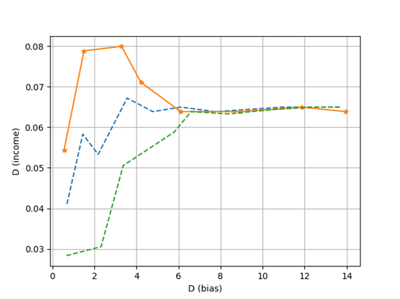
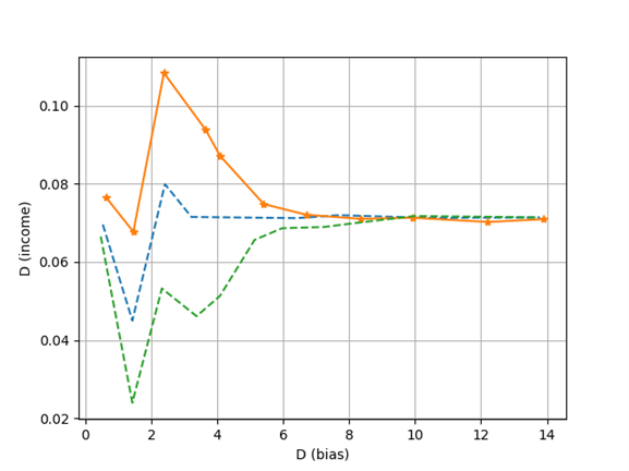
When analyzing the VAR model, the impulse response function can be used to analyze the dynamic influence between the model variables[17, 18]. The impulse response function is more practical than parameter estimation. In order to see the dynamic relationship between \(D\left( {{\text{income}}} \right)\) , \(D\left( {\operatorname{int} {\text{ernet}}} \right)\) , and \(D\left( {{\text{basis}}} \right)\), the impulse response function is drawn as shown in Figure 3 and 4. In Figures 3 and 4, the horizontal axis represents the number of lag periods (unit: year) of the shock effect, the vertical axis represents the annual increase in the basic subsistence consumption expenditure of residents, and the solid line indicates the impact of each shock variable on the basic subsistence consumption expenditure of residents [19]. The degree of response to the annual increments, the dotted line represents plus or minus two standard deviations off the band. Figure 3. The impulse response of \(D\left( {{\text{basis}}} \right)\) to \(D\left( {{\text{income}}} \right)\) According to Figure 3, it can be seen that when a positive impact is given to the annual increase of residents’ income, the annual increase of residents’ basic subsistence consumption expenditure will not increase for a period of time. After the fluctuation, it decreases rapidly, and finally tends to 0. According to Figure 4, when a positive impact is given to the annual increase in the scale of consumer finance lending in the agricultural economy, the annual increase in the basic subsistence consumption expenditure of residents first increases and then decreases, and then increases and finally decreases and tends to zero. It can also be seen that the annual increment of residents’ basic subsistence consumption expenditure is more sensitive to the impulse response of the annual increment of the agricultural economy’s consumer finance lending scale.
The impact on different types of residents’ consumption expenditure, and then analyze the impact of residents’ income, agricultural economy and consumer finance on residents’ consumption upgrade. The results show that: First, compared with residents’ income, the growth of residents’ basic subsistence consumption expenditure and the growth of residents’ enjoyment consumption expenditure are more sensitive to the development of agricultural economy and consumer finance. Second, from the perspective of contribution, compared with residents’ income, the development of agricultural economy and consumer finance has a higher final contribution to the growth of residents’ basic subsistence consumption expenditure and the growth of residents’ enjoyment consumption expenditure; Compared with the expenditure, the growth of the consumption finance scale of the agricultural economy has a higher final contribution to the growth of the enjoyment consumption expenditure of the residents’ development.
This work was supported by Research on the mechanism,measurement and path of digital technology driving the high-quality development of the real economy (HB21YJ033), and Research on the Mechanism, Measurement and Policy of Beijing-Tianjin-Hebei “New Infrastructure” to Promote Economic Growth (HB23LJ004).